Learning with Missing Features

Abstract

We introduce new online and batch algorithms that are robust to data with missing features, a situation that arises in many practical applications. In the online setup, we allow for the comparison hypothesis to change as a function of the subset of features that is observed on any given round, extending the standard setting where the comparison hypothesis is fixed throughout. In the batch setup, we present a convex relaxation of a non-convex problem to jointly estimate an imputation function, used to fill in the values of missing features, along with the classification hypothesis. We prove regret bounds in the online setting and Rademacher complexity bounds for the batch i.i.d. setting. The algorithms are tested on several UCI datasets, showing superior performance over baseline imputation methods.

1 Introduction

Standard learning algorithms assume that each training example is fully observed and doesn’t suffer any corruption. However, in many real-life scenarios, training and test data often undergo some form of corruption. We consider settings where all the features might not be observed in every example, allowing for both adversarial and stochastic feature deletion models. Such situations arise, for example, in medical diagnosis—predictions are often desired using only a partial array of medical measurements due to time or cost constraints. Survey data are often incomplete due to partial non-response of participants. Vision tasks routinely need to deal with partially corrupted or occluded images. Data collected through multiple sensors, such as multiple cameras, is often subject to the sudden failure of a subset of the sensors.

In this work, we design and analyze learning algorithms that address these examples of learning with missing features. The first setting we consider is online learning where both examples and missing features are chosen in an arbitrary, possibly adversarial, fashion. We define a novel notion of regret suitable to the setting and provide an algorithm which has a provably bounded regret on the order of $O(\sqrt{T})$, where $T$ is the number of examples. The second scenario is batch learning, where examples and missing features are drawn according to a fixed and unknown distribution. We design a learning algorithm which is guaranteed to globally optimize an intuitive objective function and which also exhibits a generalization error on the order of $O(\sqrt{d/T})$, where $d$ is the data dimension.

Both algorithms are also explored empirically across several publicly available datasets subject to various artificial and natural types of feature corruption. We find very encouraging results, indicating the efficacy of the suggested algorithms and their superior performance over baseline methods.

Learning with missing or corrupted features has a long history in statistics [14, 10], and has recieved recent attention in machine learning [9, 15, 5, 7]. Imputation methods (see [14, 15, 10]) fill in missing values, generally independent of any learning algorithm, after which standard algorithms can be applied to the data. Better performance might be expected, though, by learning the imputation and prediction functions simultaneously. Previous works [15] address this issue using EM, but can get stuck in local optima and do not have strong theoretical guarantees. Our work also is different from settings where features are missing only at test time [9, 11], settings that give access to noisy versions of all the features [6] or settings where observed features are picked by the algorithm [5].

Section 2 introduces both the general online and batch settings. Sections 3 and 4 detail the algorithms and theoretical results within the online and batch settings resp. Empirical results are presented in Section 5.

2 The Setting

In our setting it will be useful to denote a training instance ${\mathbf{x}}_{t}\in\mathbb{R}^{d}$ and prediction $y_{t}$, as well as a corruption vector ${\mathbf{z}}_{t}\in\{0,1\}^{d}$, where

$$[{\mathbf{z}}_{t}]_{i}=\left\{\begin{array}[]{cl}0&\mbox{if feature $i$ is not observed,}\\ 1&\mbox{if feature $i$ is observed.}\end{array}\right.$$

We will discuss as specific examples both classification problems where $y_{t}\in\{-1,1\}$ and regression problems where $y_{t}\in\mathbb{R}$. The learning algorithm is given the corruption vector ${\mathbf{z}}_{t}$ as well as the corrupted instance,

$${\mathbf{x}}_{t}^{\prime}={\mathbf{x}}_{t}\circ{\mathbf{z}}_{t}\,,$$

where $\circ$ denotes the component-wise product between two vectors. Note that the training algorithm is never given access to ${\mathbf{x}}_{t}$, however it is given ${\mathbf{z}}_{t}$, and so has knowledge of exactly which coordinates have been corrupted. The following subsections explain the online and batch settings respectively, as well as the type of hypotheses that are considered in each.

2.1 Online learning with missing features

In this setting, at each time-step $t$ the learning algorithm is presented with an arbitrarily (possibly adversarially) chosen instance $({\mathbf{x}}_{t}^{\prime},{\mathbf{z}}_{t})$ and is expected to predict $y_{t}$. After prediction, the label is then revealed to the learner which then can update its hypothesis.

A natural question to ask is what happens if we simply ignore the distinction between ${\mathbf{x}}^{\prime}_{t}$ and ${\mathbf{x}}_{t}$ and just run an online learning algorithm on this corrupted data. Indeed, doing so would give a small bound on regret:

$$R(T,\ell)=\sum_{t=1}^{T}\ell(\langle{\mathbf{w}}_{t},{\mathbf{x}}_{t}^{\prime}\rangle,y_{t})-\inf_{{\mathbf{w}}\in\mathcal{W}}\sum_{t=1}^{T}\ell(\langle{\mathbf{w}},{\mathbf{x}}_{t}^{\prime}\rangle,y_{t})\,,$$ (1)

with respect to a convex loss function $\ell$ and for any convex compact subset $\mathcal{W}\subseteq\mathbb{R}^{d}$. However, any fixed weight vector ${\mathbf{w}}$ in the second term might have a very large loss, making the regret guarantee useless—both the learner and the comparator have a large loss making the difference small. For instance, assume one feature perfectly predicts the label, while another one only predicts the label with 80% accuracy, and $\ell$ is the quadratic loss. It is easy to see that there is no fixed ${\mathbf{w}}$ that will perform well on both examples where the first feature is observed and examples where the first feature is missing but the second one is observed.

To address the above concerns, we consider using a linear corruption-dependent hypothesis which is permitted to change as a function of the observed corruption ${\mathbf{z}}_{t}$. Specifically, given the corrupted instance and corruption vector, the predictor uses a function ${\mathbf{w}}_{t}(\cdot):\{0,1\}^{d}\to\mathbb{R}^{d}$ to choose a weight vector, and makes the prediction $\widehat{y}_{t}=\langle{\mathbf{w}}_{t}({\mathbf{z}}_{t}),{\mathbf{x}}_{t}^{\prime}\rangle$. In order to provide theoretical guarantees, we will bound the following notion of regret,

$$\!\!\!\!\!\!R^{z}(T,\ell)\!=\!\!\!\sum_{t=1}^{T}\!\ell(\langle{\mathbf{w}}_{t},{\mathbf{x}}_{t}^{\prime}\rangle,y_{t})-\!\!\inf_{{\mathbf{w}}\in\mathcal{W}}\!\sum_{t=1}^{T}\!\ell(\langle{\mathbf{w}}({\mathbf{z}}_{t}),{\mathbf{x}}_{t}^{\prime}\rangle,y_{t}),$$ (2)

where it is implicit that ${\mathbf{w}}_{t}$ also depends on ${\mathbf{z}}_{t}$ and $\mathcal{W}$ now consists of corruption-dependent hypotheses. Similar definitions of regret have been looked at in the setting learning with side information [8, 12], but our special case admits stronger results in terms of both upper and lower bounds. In the most general case, we may consider $\mathcal{W}$ as the class of all functions which map $\{0,1\}^{d}\to\mathbb{R}^{d}$, however we show this can lead to an intractable learning problem. This motivates the study of interesting subsets of this most general function class. This is the main focus of Section 3.

2.2 Batch learning with missing features

In the setup of batch learning with i.i.d. data, examples $({\mathbf{x}}_{t},{\mathbf{z}}_{t},y_{t})$ are drawn according to a fixed but unknown distribution and the goal is to choose a hypothesis that minimizes the expected error, with respect to an appropriate loss function $\ell$: ${\mathbf{E}}_{{\mathbf{x}}_{t},{\mathbf{z}}_{t},y_{t}}[\ell(h({\mathbf{x}}_{t},{\mathbf{z}}_{t}),y_{t})]$.

The hypotheses $h$ we consider in this scenario will be inspired by imputation-based methods prevalent in statistics literature used to address the problem of missing features [14]. An imputation mapping is a function used to fill in unobserved features using the observed features, after which the completed examples can be used for prediction. In particular, if we consider an imputation function ${\boldsymbol{\phi}}:\mathbb{R}^{d}\times\{0,1\}^{d}\to\mathbb{R}^{d}$, which is meant to fill missing feature values, and a linear predictor ${\mathbf{w}}\in\mathbb{R}^{d}$, we can parameterize a hypothesis with these two function $h_{{\boldsymbol{\phi}},{\mathbf{w}}}({\mathbf{x}}^{\prime}_{t},{\mathbf{z}}_{t})=\langle{\mathbf{w}},{\boldsymbol{\phi}}({\mathbf{x}}^{\prime}_{t},{\mathbf{z}}_{t})\rangle$.

It is clear that the multiplicative interaction between ${\mathbf{w}}$ and ${\boldsymbol{\phi}}$ will make most natural formulations non-convex, and we elaborate more on this in Section 4. In the i.i.d. setting, the natural quantity of interest is the generalization error of our learned hypothesis. We provide a Rademacher complexity bound on the class of ${\mathbf{w}},{\boldsymbol{\phi}}$ pairs we use, thereby showing that any hypothesis with a small empirical error will also have a small expected loss. The specific class of hypotheses and details of the bound are presented in Section 4. Furthermore, the reason as to why an imputation-based hypothesis class is not analyzed in the more general adversarial setting will also be explained in that section.

3 Online Corruption-Based Algorithm

In this section, we consider the class of corruption-dependent hypotheses defined in Section 2.1. Recall the definition of regret (2), which we wish to control in this framework, and of the comparator class of functions $\mathcal{W}\subseteq\{0,1\}^{d}\to\mathbb{R}^{d}$. It is clear that the function class $\mathcal{W}$ is much richer than the comparator class in the corruption-free scenario, where the best linear predictor is fixed for all rounds. It is natural to ask if it is even possible to prove a non-trivial regret bound over this richer comparator class $\mathcal{W}$. In fact, the first result of our paper provides a lower bound on the minimax regret when the comparator is allowed to pick arbitrary mappings, i.e. the set $\mathcal{W}$ contains all mappings. The result is stated in terms of the minimax regret under the loss function $\ell$ under the usual (corruption-free) definition (1):

$$R^{*}(T,\ell)=\inf_{{\mathbf{w}}_{1}\in\mathcal{W}}\sup_{({\mathbf{x}}_{1},{\mathbf{z}}_{1},y_{1})}\cdots\inf_{{\mathbf{w}}_{T}\in\mathcal{W}}\sup_{({\mathbf{x}}_{T},{\mathbf{z}}_{T},y_{T})}R(T,\ell)$$

Proposition 1

If $\mathcal{W}=\{0,1\}^{d}\to\mathbb{R}^{d}$ the minimax value of the corruption dependent regret for any loss function $\ell$ is lower bounded as

$$\inf_{{\mathbf{w}}_{1}\in\mathcal{W}}\sup_{({\mathbf{x}}_{1},{\mathbf{z}}_{1},y_{1})}\cdots\inf_{{\mathbf{w}}_{T}\in\mathcal{W}}\sup_{({\mathbf{x}}_{T},{\mathbf{z}}_{T},y_{T})}\!\!\!R^{z}(T,\ell)\\ \qquad\qquad\qquad\qquad=\Omega\left(2^{d/2}R^{*}\left(\frac{T}{2^{d/2}},\ell\right)\right).$$

This proposition (the proof of which appears in the appendix [17]) shows that the minimax regret is lower bounded by a term that is exponential in the dimensionality of the learning problem. For most non-degenerate convex and Lipschitz losses, $R^{*}(T,\ell)=\Omega(\sqrt{T})$ without further assumptions (see e.g. [1]) which yields a $\Omega(2^{d/4}\sqrt{T})$ lower bound. The bound can be further strengthened to $\Omega(2^{d/2}\sqrt{T})$ for linear losses which is unimprovable since it is achieved by solving the classification problem corresponding to each pattern independently.

Thus, it will be difficult to achieve a low regret against arbitrary maps from $\{0,1\}^{d}$ to $\mathbb{R}^{d}$. In the following section we consider a restricted function class and show that a mirror-descent algorithm can achieve regret polynomial in $d$ and sub-linear in $T$, implying that the average regret is vanishing.

3.1 Linear Corruption-Dependent Hypotheses

Here we analyze a corruption-dependent hypothesis class that is parametrized by a matrix ${\mathbf{A}}\in\mathbb{R}^{d\times k}$, where $k$ may be a function of $d$. In the simplest case of $k=d$, the parametrization looks for weights ${\mathbf{w}}({\mathbf{z}}_{t})$ that depend linearly on the corruption vector ${\mathbf{z}}_{t}$. Defining ${\mathbf{w}}_{{\mathbf{A}}}({\mathbf{z}}_{t})={\mathbf{A}}{\mathbf{z}}_{t}$ achieves this, and intuitively this allows us to capture how the presence or absence of one feature affects the weight of another feature. This will be clarified further in the examples.

In general, the matrix ${\mathbf{A}}$ will be $d\times k$, where $k$ will be determined by a function ${\boldsymbol{\psi}}({\mathbf{z}}_{t})\in\{0,1\}^{k}$ that maps ${\mathbf{z}}_{t}$ to a possibly higher dimension space. Given, a fixed ${\boldsymbol{\psi}}$, the explicit parameterization in terms of ${\mathbf{A}}$ is,

$${\mathbf{w}}_{{\mathbf{A}},{\boldsymbol{\psi}}}({\mathbf{z}}_{t})={\mathbf{A}}{\boldsymbol{\psi}}({\mathbf{z}}_{t})\,.$$ (3)

In what follows, we drop the subscript from ${\mathbf{w}}_{{\mathbf{A}},{\boldsymbol{\psi}}}$ in order to simplify notation. Essentially this allows us to introduce non-linearities as a function of the corruption vector, but the non-linear transform is known and fixed throughout the learning process. Before analyzing this setting, we give a few examples and intuition as to why such a parametrization is useful. In each example, we will show how there exists a choice of a matrix ${\mathbf{A}}$ that captures the specific problem’s assumptions. This implies that the fixed comparator can use this choice in hindsight, and by having a low regret, our algorithm would implicitly learn a hypothesis close to this reasonable choice of ${\mathbf{A}}$.

3.1.1 Corruption-free special case

We start by noting that in the case of no corruption (i.e. $\forall t,{\mathbf{z}}_{t}={\mathbf{1}}$) a standard linear hypothesis model can be cast within the matrix based framework by defining ${\boldsymbol{\psi}}({\mathbf{z}}_{t})=1$ and learning ${\mathbf{A}}\in\mathbb{R}^{d\times 1}$.

3.1.2 Ranking-based parameterization

One natural method for classification is to order the features by their predictive power, and to weight features proportionally to their ranking (in terms of absolute value; that is, the sign of weight depends on whether the correlation with the label is positive or negative). In the corrupted features setting, this naturally corresponds to taking the available features at any round and putting more weight on the most predictive observed features. This is particularly important while using margin-based losses such as the hinge loss, where we want the prediction to have the right sign and be large enough in magnitude.

Our parametrization allows such a strategy when using a simple function ${\boldsymbol{\psi}}({\mathbf{z}}_{t})={\mathbf{z}}_{t}$. Without loss of generality, assume that the features are arranged in decreasing order of discriminative power (we can always rearrange rows and columns of ${\mathbf{A}}$ if they’re not). We also assume positive correlations of all features with the label; a more elaborate construction works for ${\mathbf{A}}$ when they’re not. In this case, consider the parameter matrix and the induced classification weights

$$[{\mathbf{A}}]_{i,j}=\left\{\begin{array}[]{rl}1,&j=i\\ -\frac{1}{d},&j<i\\ 0,&j>i\end{array}\right.\!\!,~{}~{}[{\mathbf{w}}({\mathbf{z}}_{t})]_{i}\!=\![{\mathbf{z}}_{t}]_{i}\biggr{(}1-\!\!\!\!\!\sum_{\begin{subarray}{c}j<i:\\ [{\mathbf{z}}_{t}]_{j}=1\end{subarray}}\frac{1}{d}\biggr{)}.$$

Thus, for all $i<j$ such that $[{\mathbf{z}}_{t}]_{i}=[{\mathbf{z}}_{t}]_{j}=1$ we have $[{\mathbf{w}}({\mathbf{z}}_{t})]_{i}\geq[{\mathbf{w}}({\mathbf{z}}_{t})]_{j}$. The choice of 1 for diagonals and $1/d$ for off-diagonals is arbitrary and other values might also be picked based on the data sequence $({\mathbf{x}}_{t},{\mathbf{z}}_{t},y_{t})$. In general, features are weighted monotonically with respect to their discriminative power with signs based on correlations with the label.

3.1.3 Feature group based parameterization

Another class of hypotheses that we can define within this framework are those restricted to consider up to $p$-wise interactions between features for some constant $0<p\leq d$. In this case, we index the $k=\sum_{i=1}^{p}\binom{d}{i}=O\big{(}(\frac{d}{p})^{p}\big{)}$ unique subsets of features of size up to $p$. Then define $[{\boldsymbol{\psi}}({\mathbf{z}}_{t})]_{j}=1$ if the corresponding subset $j$ is uncorrupted by ${\mathbf{z}}_{t}$ and equal to $0$ otherwise. An entry $[{\mathbf{A}}]_{i,j}$ now specifies the importance of feature $j$, assuming that at least the subset $i$ is present. Such a model would, for example, have the ability to capture the scenario of a feature that is only discriminative in the presence of some $p-1$ other features. For example, we can generalize the ranking example from above to impose a soft ranking on groups of features.

3.1.4 Corruption due to failed sensors

A common scenario for missing features arises in applications involving an array of measurements, for example, from a sensor network, wireless motes, array of cameras or CCDs, where each sensor is bound to fail occasionally. The typical strategy for dealing with such situations involves the use of redundancy. For instance, if a sensor fails, then some kind of an averaged measurement from the neighboring sensors might provide a reasonable surrogate for the missing value.

It is possible to design a choice of ${\mathbf{A}}$ matrix for the comparator that only uses the local measurement when it is present, but uses an averaged approximation based on some fixed averaging distribution on neighboring features when the local measurement is missing. For each feature, we consider a probability distribution $p_{i}$ which specifies the averaging weights to be used when approximating feature $i$ using neighboring observations. Let ${\mathbf{w}}^{*}$ be the weight vector that the comparator would like to use if all the features were present. Then, with ${\boldsymbol{\psi}}({\mathbf{z}})={\mathbf{z}}$ and for $j\neq i$ we define,

$$[{\mathbf{A}}]_{i,i}={\mathbf{w}}^{*}_{i}+\sum_{j\neq i}{\mathbf{w}}^{*}_{j}p_{ji},\quad[{\mathbf{A}}]_{i,j}=-{\mathbf{w}}^{*}_{j}p_{ji}.$$ (4)

Thus, say only feature $k$ is missing, we still have ${{\mathbf{x}}^{\prime}}_{t}^{\top}{\mathbf{A}}{\mathbf{z}}_{t}=\sum_{i,j}[{\mathbf{x}}^{\prime}_{t}]_{i}[{\mathbf{z}}_{t}]_{j}[{\mathbf{A}}]_{i,j}=\sum_{i\neq k,j\neq k}[{\mathbf{x}}_{t}]_{i}[{\mathbf{A}}]_{i,j}=\sum_{i\neq k}[{\mathbf{x}}_{t}]_{i}[{\mathbf{w}}^{*}]_{i}+[{\mathbf{w}}^{*}]_{k}\sum_{i\neq k}[{\mathbf{x}}_{t}]_{i}p_{ki}$, where by assumption $\sum_{i\neq k}[{\mathbf{x}}_{t}]_{i}p_{ki}\approx[{\mathbf{x}}_{t}]_{k}$.

Of course, the averaging in such applications is typically local, and we expect each sensor to put large weights only on neighboring sensors. This can be specified via a neighborhood graph, where nodes $i$ and $j$ have an edge if $j$ is used to predict $i$ when feature $i$ is not observed and vice versa. From the construction (4) it is clear that the only off-diagonal entries that are non-zero would correspond to the edges in the neighborhood graph. Thus we can even add this information to our algorithm and constrain several off-diagonal elements to be zero, thereby restricting the complexity of the problem.

3.2 Matrix-Based Algorithm and Regret

We use a standard mirror-descent style algorithm [16, 3] in the matrix based parametrization described above. It is characterized by a strongly convex regularizer $\mathcal{R}~{}:~{}\mathbb{R}^{d\times k}\to\mathbb{R}$, that is

$$\mathcal{R}({\mathbf{A}})\geq\mathcal{R}({\mathbf{B}})+\langle\nabla\mathcal{R}({\mathbf{B}}),{\mathbf{A}}-{\mathbf{B}}\rangle_{F}+\frac{1}{2}\|{\mathbf{A}}-{\mathbf{B}}\|^{2}~{}~{}\forall{\mathbf{A}},{\mathbf{B}}\!\in\!\mathcal{A},\vspace{-0.2cm}$$

for some norm $\|\cdot\|$ and where $\langle{\mathbf{A}},{\mathbf{B}}\rangle_{F}=\mathrm{Tr}({\mathbf{A}}^{\top}{\mathbf{B}})$ is the trace inner product. An example is the squared Frobenius norm $\mathcal{R}({\mathbf{A}})=\frac{1}{2}\|{\mathbf{A}}\|_{F}^{2}$. For any such function, we can define the associated Bregman divergence

$$D_{\mathcal{R}}({\mathbf{A}},{\mathbf{B}})=\mathcal{R}({\mathbf{A}})-\mathcal{R}({\mathbf{B}})-\langle\nabla\mathcal{R}({\mathbf{B}}),{\mathbf{A}}-{\mathbf{B}}\rangle_{F}.$$

We assume $\mathcal{A}$ is a convex subset of $\mathbb{R}^{d\times k}$, which could encode constraints such as some off-diagonal entries being zero in the setup of Section 3.1.4. To simplify presentation in what follows, we will use the shorthand $\ell_{t}({\mathbf{A}})=\ell(\langle{\mathbf{A}}{\boldsymbol{\psi}}({\mathbf{z}}_{t}),{\mathbf{x}}^{\prime}_{t}\rangle,y_{t})$. The algorithm initializes with any ${\mathbf{A}}_{0}\in\mathcal{A}$ and updates

$${\mathbf{A}}_{t+1}\!\!=\!\arg\min_{{\mathbf{A}}\in\mathcal{A}}\left\{\eta_{t}\langle\nabla\ell_{t}({\mathbf{A}}_{t}),{\mathbf{A}}\rangle_{F}\!+\!D_{\mathcal{R}}({\mathbf{A}},{\mathbf{A}}_{t})\right\}$$ (5)

If $\mathcal{A}=\mathbb{R}^{d\times k}$ and $\mathcal{R}({\mathbf{A}})=\frac{1}{2}\|{\mathbf{A}}\|_{F}^{2}$, the update simplifies to gradient descent ${\mathbf{A}}_{t+1}={\mathbf{A}}_{t}-\eta_{t}\nabla\ell_{t}({\mathbf{A}}_{t})$.

Our main result of this section is a guarantee on the regret incurred by Algorithm (5). The proof follows from standard arguments (see e.g. [16, 4]). Below, the dual norm is defined as $\|{\mathbf{V}}\|_{*}=\sup_{{\mathbf{U}}:\|{\mathbf{U}}\|\leq 1}\langle{\mathbf{U}},{\mathbf{V}}\rangle_{F}$.

Theorem 1

Let $\mathcal{R}$ be strongly convex with respect to a norm $\|\cdot\|$ and $\|\nabla\ell_{t}({\mathbf{A}})\|_{*}\leq G$, then Algorithm 5 with learning rate $\eta_{t}=\frac{R}{G\sqrt{T}}$ exhibits the following regret upper bound compared to any ${\mathbf{A}}$ with $\|{\mathbf{A}}\|\leq R$,

$$\sum_{t=1}^{T}\!\ell(\langle{\mathbf{A}}_{t}{\mathbf{z}}_{t},{\mathbf{x}}_{t}^{\prime}\rangle,y_{t})-\!\!\inf_{{\mathbf{A}}\in\mathcal{A}}\sum_{t=1}^{T}\!\ell(\langle{\mathbf{A}}{\mathbf{z}}_{t},{\mathbf{x}}_{t}^{\prime}\rangle,y_{t})\leq 3RG\sqrt{T}.$$

4 Batch Imputation Based Algorithm

Recalling the setup of Section 2.2, in this section we look at imputation mappings of the form

$${\boldsymbol{\phi}}_{{\mathbf{M}}}({\mathbf{x}}^{\prime},{\mathbf{z}})={\mathbf{x}}^{\prime}+\operatorname{diag}(1-{\mathbf{z}}){\mathbf{M}}^{\top}{\mathbf{x}}^{\prime}\,.$$ (6)

Thus we retain all the observed entries in the vector ${\mathbf{x}}^{\prime}$, but for the missing features that are predicted using a linear combination of the observed features and where the $i_{th}$ column of ${\mathbf{M}}$ encodes the averaging weights for the $i_{th}$ feature. Such a linear prediction framework for features is natural. For instance, when the data vectors ${\mathbf{x}}$ are Gaussian, the conditional expectation of any feature given the other features is a linear function. The predictions are now made using the dot product

$$\langle{\mathbf{w}},{\boldsymbol{\phi}}({\mathbf{x}}^{\prime},{\mathbf{z}})\rangle=\langle{\mathbf{w}},{\mathbf{x}}^{\prime}\rangle+\langle{\mathbf{w}},\operatorname{diag}(1-{\mathbf{z}}){\mathbf{M}}^{\top}{\mathbf{x}}^{\prime}\rangle,$$

where we would like to estimate ${\mathbf{w}},{\mathbf{M}}$ based on the data samples. From a quick inspection of the resulting learning problem, it becomes clear that optimizing over such a hypothesis class leads to a non-convex problem. The convexity of the loss plays a critical role in the regret framework of online learning, which is why we restrict ourselves to a batch i.i.d. setting here.

In the sequel we will provide a convex relaxation to the learning problem resulting from the parametrization (6). While we can make this relaxation for natural loss functions in both classification and regression scenarios, we restrict ourselves to a linear regression setting here as the presentation for that example is simpler due to the existence of a closed form solution for the ridge regression problem.

In what follows, we consider only the corrupted data and thus simply denote corrupted examples as ${\mathbf{x}}_{i}$. Let ${\mathbf{X}}$ denote the matrix with $i_{th}$ row equal to ${\mathbf{x}}_{i}$ and similarly define ${\mathbf{Z}}$ as the matrix with $i_{th}$ row equal to ${\mathbf{z}}_{i}$. It will also be useful to define $\overline{{\mathbf{Z}}}={\mathbf{1}}{\mathbf{1}}^{\top}-{\mathbf{Z}}$ and $\overline{{\mathbf{z}}}_{i}={\mathbf{1}}-{\mathbf{z}}_{i}$ and finally let $\overline{{\mathbf{Z}}}_{i}=\operatorname{diag}(\overline{{\mathbf{z}}}_{i})$.

4.1 Imputed Ridge Regression (IRR)

In this section we will consider a modified version of the ridge regression (RR) algorithm, robust to missing features. The overall optimization problem we are interested in is as follows,

$$\min_{\{{\mathbf{w}},{\mathbf{M}}:\|{\mathbf{M}}\|_{F}\leq\gamma\}}\!\frac{\lambda}{2}\|{\mathbf{w}}\|^{2}\!+\!\frac{1}{T}\sum_{i=1}^{T}\!\big{(}y_{i}\!-\!{\mathbf{w}}^{\top}\!({\mathbf{x}}_{i}\!+\!\overline{{\mathbf{Z}}}_{i}{\mathbf{M}}^{\top}{\mathbf{x}}_{i})\big{)}^{2}$$ (7)

where the hypothesis ${\mathbf{w}}$ and imputation matrix ${\mathbf{M}}$ are simultaneously optimized. In order to bound the size of the hypothesis set, we have introduced the constraint $\|{\mathbf{M}}\|_{F}^{2}\leq\gamma^{2}$ that bounds the Frobenius norm of the imputation matrix. The global optimum of the problem as presented in (7) cannot be easily found as it is not jointly convex in both ${\mathbf{w}}$ and ${\mathbf{M}}$. We next present a convex relaxation of the formulation (7). The key idea is to take a dual over ${\mathbf{w}}$ but not ${\mathbf{M}}$, so that we have a saddle-point problem in the dual vector ${\boldsymbol{\alpha}}$ and ${\mathbf{M}}$. The resulting saddle point problem, while being concave in ${\boldsymbol{\alpha}}$ is still not convex in ${\mathbf{M}}$. At this step we introduce a new tensor ${\mathbf{N}}\in\mathbb{R}^{d\times d\times d}$, where $[{\mathbf{N}}]_{i,j,k}=[{\mathbf{M}}]_{i,k}[{\mathbf{M}}]_{j,k}$. Finally we drop the non-convex constraint relating ${\mathbf{M}}$ and ${\mathbf{N}}$ replacing it with a matrix positive semidefiniteness constraint.

Before we can describe the convex relaxation, we need one more piece of notation. Given a matrix ${\mathbf{M}}$ and a tensor ${\mathbf{N}}$, we define the matrix ${\mathbf{K}}_{{\mathbf{M}}{\mathbf{N}}}\in\mathbb{R}^{T\times T}$

$$[{\mathbf{K}}_{{\mathbf{M}}{\mathbf{N}}}]_{i,j}={\mathbf{x}}_{i}^{\top}{\mathbf{x}}_{j}+{\mathbf{x}}_{i}^{\top}{\mathbf{M}}\overline{{\mathbf{Z}}}_{i}{\mathbf{x}}_{j}+{\mathbf{x}}_{i}^{\top}\overline{{\mathbf{Z}}}_{j}{\mathbf{M}}^{\top}{\mathbf{x}}_{j}\\ +\sum_{k=1}^{d}[\overline{{\mathbf{z}}}_{i}]_{k}[\overline{{\mathbf{z}}}_{j}]_{k}{\mathbf{x}}_{i}^{\top}{\mathbf{N}}_{k}{\mathbf{x}}_{j}\,.$$ (8)

The following proposition gives the convex relaxation of the problem (7) that we refer to as Imputed Ridge Regression (IRR) and which includes a strictly larger hypothesis than the $({\mathbf{w}},{\mathbf{M}})$ pairs with which we began.

Proposition 2

The following semi-definite programming optimization problem provides a convex relaxation to the non-convex problem (7):

$$\min_{\begin{subarray}{c}t,~{}{\mathbf{M}}:\|{\mathbf{M}}\|^{2}_{F}\leq\gamma^{2}\\ {\mathbf{N}}:\sum_{k}\|{\mathbf{N}}_{k}\|_{F}^{2}\leq\gamma^{4}\end{subarray}}t$$ (9)

$$\mathrm{s.t.}~{}~{}\left[\begin{array}[]{cc}{\mathbf{K}}_{{\mathbf{M}}{\mathbf{N}}}+\lambda T{\mathbf{I}}&{\mathbf{y}}\\ {\mathbf{y}}^{\top}&t\end{array}\right]\succeq 0,~{}~{}{\mathbf{K}}_{{\mathbf{M}}{\mathbf{N}}}\succeq 0\,.$$ (12)

The proof is deferred to the appendix for lack of space. The main idea is to take the quadratic form that arises in the dual formulation of (7) with the matrix ${\mathbf{K}}_{\mathbf{M}}$,

$$\!\!\!\!\!\![{\mathbf{K}}_{{\mathbf{M}}}]_{i,j}\!=\!{\mathbf{x}}_{i}^{\top}{\mathbf{x}}_{j}\!+\!{\mathbf{x}}_{i}^{\top}{\mathbf{M}}\overline{{\mathbf{Z}}}_{i}{\mathbf{x}}_{j}\!+\!{\mathbf{x}}_{i}^{\top}\overline{{\mathbf{Z}}}_{j}{\mathbf{M}}^{\top}{\mathbf{x}}_{j}\!+\!{\mathbf{x}}_{i}^{\top}{\mathbf{M}}\overline{{\mathbf{Z}}}_{i}\overline{{\mathbf{Z}}}_{j}{\mathbf{M}}^{\top}{\mathbf{x}}_{j}\!,$$

and relax it to the matrix ${\mathbf{K}}_{{\mathbf{M}}{\mathbf{N}}}$ (8). The constraint involving positive semidefiniteness of ${\mathbf{K}}_{{\mathbf{M}}{\mathbf{N}}}$ is needed to ensure the convexity of the relaxed problem. The norm constraint on ${\mathbf{N}}$ is a consequence of the norm constraint on ${\mathbf{M}}$.

One tricky issue with relaxations is using the relaxed solution in order to find a good solution to the original problem. In our case, this would correspond to finding a good ${\mathbf{w}},{\mathbf{M}}$ pair for the primal problem (7). We bypass this step, and instead directly define the prediction on any point $({\mathbf{x}}_{0},{\mathbf{z}}_{0})$ as:

$$\sum_{i=1}^{T}\alpha_{i}({\mathbf{x}}_{i}^{\top}{\mathbf{x}}_{0}+{\mathbf{x}}_{i}^{\top}{\mathbf{M}}\overline{{\mathbf{Z}}}_{i}{\mathbf{x}}_{0}+{\mathbf{x}}_{i}^{\top}\overline{{\mathbf{Z}}}_{0}{\mathbf{M}}^{\top}{\mathbf{x}}_{0}\\ +\sum_{k=1}^{d}[\overline{{\mathbf{z}}}_{i}]_{k}[\overline{{\mathbf{z}}}_{0}]_{k}{\mathbf{x}}_{i}^{\top}{\mathbf{N}}_{k}{\mathbf{x}}_{0}).$$ (13)

Here, ${\boldsymbol{\alpha}},{\mathbf{M}},{\mathbf{N}}$ are solutions to the saddle-point problem

$$\min_{\begin{subarray}{c}{\mathbf{M}}:\|{\mathbf{M}}\|_{F}\leq\gamma\\ {\mathbf{N}}:\sum_{k}\|{\mathbf{N}}_{k}\|_{F}^{2}\leq\gamma^{4}\end{subarray}}\!\!\!\!\!\max_{\boldsymbol{\alpha}}2{\boldsymbol{\alpha}}^{\top}{\mathbf{y}}\!-\!{\boldsymbol{\alpha}}^{\top}({\mathbf{K}}_{{\mathbf{M}}{\mathbf{N}}}\!+\!\lambda T{\mathbf{I}}){\boldsymbol{\alpha}}\,.$$ (14)

We start by noting that the above optimization problem is equivalent to the one in Proposition 2. The intuition behind this definition (13) is that the solution to the problem (7) has this form, with $[{\mathbf{N}}]_{i,j,k}$ replaced with $[{\mathbf{M}}]_{i,k}[{\mathbf{M}}]_{j,k}$. In the next section, we show a Rademacher complexity bound over functions of the form above to justify our convex relaxation.

4.2 Theoretical analysis of IRR

As mentioned in the previous section, we predict with a hypothesis of the form (13) rather than going back to the primal class indexed by $({\mathbf{w}},{\mathbf{M}})$ pairs. In this section, we would like to show that the new hypothesis class parametrized by ${\boldsymbol{\alpha}},{\mathbf{M}},{\mathbf{N}}$ is not too rich for the purposes of learning. To do this, we give the class of all possible hypotheses that can be the solutions to the dual problem (9) and then prove a Rademacher complexity bound over that class. The set of all possible ${\boldsymbol{\alpha}},{\mathbf{M}},{\mathbf{N}}$ triples that can be potential solutions to (9) lie in the following set

$$\!\!\!\mathcal{H}\!=\!\Bigg{\{}\!h({\mathbf{x}}_{0},{\mathbf{z}}_{0})\!\mapsto\!\!\sum_{i=1}^{T}\!\!\alpha_{i}({\mathbf{x}}_{i}^{\top}{\mathbf{x}}_{0}+{\mathbf{x}}_{i}^{\top}{\mathbf{M}}\overline{{\mathbf{Z}}}_{i}{\mathbf{x}}_{0}+{\mathbf{x}}_{i}^{\top}\overline{{\mathbf{Z}}}_{0}{\mathbf{M}}^{\top}{\mathbf{x}}_{0}+\\ \sum_{k=1}^{d}[\overline{{\mathbf{z}}}_{i}]_{k}[\overline{{\mathbf{z}}}_{0}]_{k}{\mathbf{x}}_{i}^{\top}{\mathbf{N}}_{k}{\mathbf{x}}_{0})\!:\!\|{\mathbf{M}}\|_{F}\!\leq\!\gamma,\|{\mathbf{N}}\|_{F}\!\leq\!\gamma^{2},\|{\boldsymbol{\alpha}}\|\!\leq\!\frac{B}{\lambda\sqrt{T}}\!\Bigg{\}}$$

The bound on $\|{\boldsymbol{\alpha}}\|$ is made implicitly in the optimization problem (assuming the training labels are bounded $\forall i,|y_{i}|\leq B$). To see this, we note that the problem (9) is obtained from (14) by using the closed-form solution of the optimal ${\boldsymbol{\alpha}}=({\mathbf{K}}_{{\mathbf{M}}{\mathbf{N}}}+\lambda T{\mathbf{I}})^{-1}{\mathbf{y}}$. Then we can bound $\|{\boldsymbol{\alpha}}\|\leq\|{\mathbf{y}}\|/\lambda_{\min}({\mathbf{K}}_{{\mathbf{M}}{\mathbf{N}}}+\lambda T{\mathbf{I}})=\frac{B\sqrt{T}}{\lambda T}$, where $\lambda_{\min}({\mathbf{A}})$ denotes the smallest eigenvalue of the matrix ${\mathbf{A}}$. Note that in general there is no linear hypothesis ${\mathbf{w}}$ that corresponds to the hypotheses in the relaxed class $\mathcal{H}$ and that we are dealing with a strictly more general function class. However, the following theorem demonstrates that the Rademacher complexity of this function class is reasonably bounded in terms of the number of training points $T$ and dimension $d$ and thereby still provides provable generalization performance [2].

Recall the Rademacher complexity of a class $\mathcal{H}$

$$\mathfrak{R}_{T}(\mathcal{H})={\mathbf{E}}_{S}{\mathbf{E}}_{{\boldsymbol{\sigma}}}\left[\frac{1}{T}\sup_{h\in\mathcal{H}}\bigg{|}\sum_{i=1}^{T}\sigma_{i}h({\mathbf{x}}_{i},{\mathbf{z}}_{i})\bigg{|}\right]\,,$$ (15)

where the inner expectation is over independent Rademacher random variables $(\sigma_{1},\ldots,\sigma_{T})$ and the outer one over a sample $S=(({\mathbf{x}}_{1},{\mathbf{z}}_{1}),\ldots,({\mathbf{x}}_{T},{\mathbf{z}}_{T}))$.

Theorem 2

If we assume a bounded regression problem $\forall y,~{}|y|\leq B$ and $\forall{\mathbf{x}},~{}\|{\mathbf{x}}\|\leq R$, then the Rademacher complexity of the hypothesis set $\mathcal{H}$ is bounded as follows,

$$\mathfrak{R}_{T}(\mathcal{H})\leq\big{(}1+\gamma+(\gamma+\gamma^{2})\sqrt{d}\big{)}\frac{BR^{2}}{\lambda\sqrt{T}}=O\bigg{(}\sqrt{\frac{d}{T}}\bigg{)}\,.$$

Due to space constraints, the proof is presented in the appendix. Theorem 2 allows us to control the gap between empirical and expected risks using standard Rademacher complexity results. Theorem 8 of [2], immediately provides the following corollary.

Corollary 3

Under the conditions of Theorem 2, for any $0<\delta\leq 1$, with probability at least $1-\delta$ over samples of size $T$, every $h\in\mathcal{H}$ satisfies

$${\mathbf{E}} [(y-h({\mathbf{x}}^{\prime},{\mathbf{z}}))^{2}]\leq\frac{1}{T}\sum_{t=1}^{T}(y_{t}-h({\mathbf{x}}^{\prime}_{t},{\mathbf{z}}_{t}))^{2}$$

$$+\frac{BR^{2}(1+\gamma)^{2}}{\lambda}\left(\frac{BR^{2}(1+\gamma)^{2}}{\lambda}\sqrt{\frac{d}{T}}+\sqrt{\frac{8\ln(2/\delta)}{T}}\right).$$

5 Empirical Results

This section presents empirical evaluation of the online matrix-based algorithm 5, as well as the Imputed Ridge Regression algorithm of Section 4.1. We use baseline methods zero-imputation and mean-imputation where the missing entries are replaced with zeros and mean estimated from observed values of those features resp. Once the data is imputed, a standard online gradient descent algorithm or ridge-regression algorithm is used. As reference, we also show the performance of a standard algorithm on uncorrupted data. The algorithms are evaluated on several UCI repository datasets, summarized in Table 1.

The thyroid dataset includes naturally corrupted/missing data. The optdigits dataset is subjected to artificial corruption by deleting a column of pixels, chosen uniformly at random from the 3 central columns of the image (each image contains 8 columns of pixels total). The remainder of the datasets are subjected to two types of artificial corruption: data-independent or data-dependent corruption. In the first case, each feature is randomly deleted independently, while the features are deleted based on thresholding values in the latter case.

dataset	$m$	$d$	$F_{I}$	$F_{D}$
abalone	4177	7	$.62\pm.08$	$.61\pm.12$
housing	20640	8	$.64\pm.08$	$.68\pm.20$
optdigits	5620	64	$.88\pm.00$	$.88\pm.00$
park	3000	20	$.58\pm.06$	$.61\pm.08$
thyroid	3163	5	$.77\pm.00$	$.77\pm.00$
splice	1000	60	$.63\pm.01$	$.66\pm.03$
wine	6497	11	$.63\pm.10$	$.69\pm.13$

Table 1: Size of dataset ($m$), features ($d$) and, the overall fraction of remaining features in the training set after data-independent ($F_{I}$) or data-dependent ($F_{D}$) corruption.

We report average error and standard deviations over 5 trials, using 1000 random training examples and corruption patterns. We tune hyper-parameters using a grid search from $2^{-12}$ to $2^{10}$. Further details and explicit corruption processes appear in the appendix.

5.1 Online Corruption Dependent Hypothesis

Here we analyze the online algorithm presented in section 3.2 using two different types of regularization. The first method simply penalizes the Frobenius norm of the parameter matrix ${\mathbf{A}}$ (frob-reg), $\mathcal{R}({\mathbf{A}})=\|{\mathbf{A}}\|_{F}^{2}$. The second method (sparse-reg) forces a sparse solution by constraining many entries of the parameter matrix equal to zero as mentioned in Section 3.1.4. We use the regularizer $\mathcal{R}({\mathbf{A}})=\gamma\|{\mathbf{A}}{\mathbf{1}}\|^{2}+\|{\mathbf{A}}\|_{F}^{2}$, where $\gamma$ is an additional tunable parameter. This choice of regularization is based on the example given in equation (4), where we would have $\|{\mathbf{A}}{\mathbf{1}}\|=\|{\mathbf{w}}^{*}\|$.

We apply these methods to the splice classification task and the optdigits dataset in several one vs. all classification tasks. For splice, the sparsity pattern used by the sparse-reg method is chosen by constraining those entries $[{\mathbf{A}}]_{i,j}$ where feature $i$ and $j$ have a correlation coefficient less than 0.2, as measured with the corrupted training sample. In the case of optdigits, only entries corresponding to neighboring pixels are allowed to be non-zero.

Figure 1 shows that, when subject to data-independent corruption, the zero imputation, mean imputation and frob-reg methods all perform relatively poorly while the sparse-reg method provides significant improvement for the splice dataset. Furthermore, we find data-dependent corruption is quite harmful to mean imputation as might be expected, while both frob-reg and sparse-reg still provide significant improvement over zero-imputation. More surprisingly, these methods also perform better than training on uncorrupted data. We attribute this to the fact that we are using a richer hypothesis function that is parametrized by the corruption vector while the standard algorithm uses only a fixed hypothesis. In Table 2 we see that the sparse-reg performs at least as well as both zero and mean imputation in all tasks and offers significant improvement in the 3-vs-all and 6-vs-all task. In this case, the frob-reg method performs comparably to sparse-reg and is omitted from the table due to space.

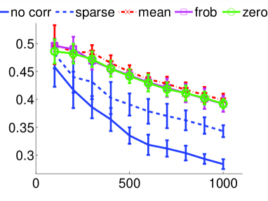
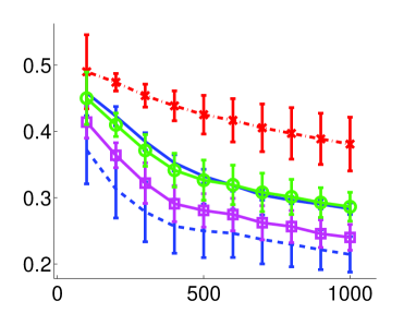
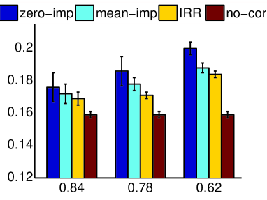
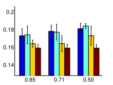
Figure 1: 0/1 loss as a function of $T$ for splice dataset with independent (top left) and dependent corruption (top right). RMSE on abalone across varying amounts of independent (bottom left) and dependent corruption (bottom right); fraction of features remaining indicated on x-axis.

	zero-imp	mean-imp	sparse-reg	no corr
2	$.035\pm.002$	$.039\pm.004$	$.033\pm.003$	$.024\pm.002$
3	$.041\pm.002$	$.043\pm.001$	$\mathbf{.039\pm.002}$	$.027\pm.003$
4	$.020\pm.002$	$.023\pm.002$	$.021\pm.001$	$.015\pm.001$
6	$.026\pm.002$	$.024\pm.002$	$\mathbf{.023\pm.002}$	$.015\pm.002$

Table 2: One-vs-all classification results on optdigits dataset (target digit in first column) with column-based corruption for 0/1 loss.

5.2 Imputed Ridge Regression

In this section we consider the performance of IRR across many datasets. We found standard SDP solvers to be quite slow for problem (9). We instead use a semi-infinite linear program (SILP) to find an approximately optimal solution (see e.g. [13] for details).

In Tables 3 and 4 we compare the performance of the IRR algorithm to zero and mean imputation as well as to standard ridge regression performance on the uncorrupted data. Here we see IRR provides improvement over zero-imputation in all cases and does at least as well as mean-imputation when dealing with data-independent corruption. For data-dependent corruption, IRR continues to perform well, while mean-imputation suffers. For this setting, we have also compared to an independent-imputation method, which imputes data using an ${\mathbf{M}}$ matrix that is trained independently of the learning algorithm. In particular the $i_{th}$ column of ${\mathbf{M}}$ is selected as the best linear predictor of the $i_{th}$ feature given the rest, i.e. the solution to: $\operatorname*{\rm argmin}_{\mathbf{v}}\sum_{k\in\mathcal{X}_{i}}([{\mathbf{x}}_{k}]_{i}-\sum_{j\neq i}[{\mathbf{x}}_{k}]_{j}[{\mathbf{v}}]_{j})^{2},$ where $\mathcal{X}_{i}$ is the set of training examples that have the $i_{th}$ feature present. Although, this method can perform better than mean-imputation, the joint optimization solution provided by IRR provides an even more significant improvement. At the bottom of Table 4 we also measure performance with thyroid which has naturally missing values. Here again IRR performs significantly better than the competitor methods. Zero-imputation is not shown due to space, but it performs uniformly worse. Figure 1 shows more detailed results for the abalone dataset across different levels of corruption and displays the consistent improvement which the IRR algorithm provides.

	zero-imp	mean-imp	IRR	no corr
A	$.199\pm.004$	$.187\pm.003$	$\mathbf{.183\pm.002}$	$.158\pm.002$
H	$.414\pm.025$	$\mathbf{.370\pm.019}$	$\mathbf{.373\pm.019}$	$.288\pm.001$
P	$.457\pm.006$	$\mathbf{.445\pm.004}$	$.451\pm.004$	$.422\pm.004$
W	$.280\pm.006$	$\mathbf{.268\pm.009}$	$\mathbf{.269\pm.008}$	$.246\pm.001$

Table 3: RMSE for various imputation methods across the datasets abalone (A), housing (H), park (P) and wine (W) when subject to data-independent corruption

	mean-imp	ind-imp	IRR	no corr
A	$.180\pm.006$	$.183\pm.012$	$\mathbf{.167\pm.011}$	$.159\pm.004$
H	$.400\pm.064$	$.363\pm.041$	$\mathbf{.326\pm.035}$	$.289\pm.001$
P	$.444\pm.008$	$.423\pm.015$	$\mathbf{.377\pm.035}$	$.422\pm.001$
W	$.264\pm.009$	$.260\pm.011$	$.256\pm.011$	$.247\pm.001$
T	$.531\pm.005$	$.528\pm.003$	$\mathbf{.521\pm.004}$	–

Table 4: RMSE for various imputation methods across the datasets abalone (A), housing (H), park (P) and wine (W) when subject to data-dependent corruption. The thyroid (T) dataset has naturally occurring missing features.

In Table 5 we see that, with respect to the column-corrupted optdigit dataset, the IRR algorithm performs significantly better than zero-imputation and mean-imputation in majority of tasks.

	zero-imp	mean-imp	IRR	no corr
2	$.352\pm.003$	$.351\pm.004$	$\mathbf{.346\pm.002}$	$.321\pm.003$
3	$.450\pm.005$	$.435\pm.004$	$\mathbf{.426\pm.005}$	$.398\pm.004$
4	$.372\pm.003$	$\mathbf{.363\pm.002}$	$\mathbf{.364\pm.003}$	$.345\pm.002$
6	$.369\pm.003$	$.360\pm.002$	$\mathbf{.353\pm.003}$	$.333\pm.003$

Table 5: RMSE (using binary labels) for one-vs-all classification on optdigits subject to column-based corruption.

6 Conclusion

We have introduced two new algorithms, addressing the problem of learning with missing features in both the adversarial online and i.i.d. batch settings. The algorithms are motivated by intuitive constructions and we also provide theoretical performance guarantees. Empirically we show encouraging initial results for online matrix-based corruption-dependent hypotheses as well as many significant results for the suggested IRR algorithm, which indicate superior performance when compared to several baseline imputation methods.

Acknowledgements

We gratefully acknowledge the support of the NSF under award DMS-0830410. AA was partially supported by an MSR PhD Fellowship. We also thank anonymous reviewers for suggesting additional references and improvements to proofs.

Appendix A Proof of Proposition 1

The strategy used here is to consider the total regret accumulated by an algorithm on several different tasks, each one indexed by a different ${\mathbf{z}}_{t}$.

First, in order to simplify the interaction between ${\mathbf{z}}_{t}$ and ${\mathbf{x}}_{t}$, suppose only the first $d/2$ coordinates of ${\mathbf{x}}_{t}$ contain information (and the rest are always set equal to 0) and assume only the last $d/2$ coordinates of ${\mathbf{z}}_{t}$ contain any information (the rest are always set equal to 1). Thus, for every one of the $2^{d/2}$ distinct values of ${\mathbf{z}}_{t}$ we associate a different independent ${\mathbf{w}}^{*}({\mathbf{z}}_{t})$, or task, which the algorithm is trying to learn.

The main intuition is that the learning problem now reduces to a multitask classification problem with $K=2^{d/2}$ different tasks. Without further assumptions, it can be shown that the minimax regret of such a multitask classification problem is as bad as solving the tasks independently.

We partition the total number of iterations $T=\sum_{i=1}^{2^{d/2}}T_{i}$, where each $T_{i}$ is the number of iterations a particular ${\mathbf{z}}_{t}$ was used by the adversary. In order to analyze the minimax regret, we can use von-Neumann duality (see e.g. [1]) to get

$$\inf_{{\mathbf{w}}_{1}}\sup_{({\mathbf{x}}_{1},{\mathbf{z}}_{1},y_{1})}\cdots\inf_{{\mathbf{w}}_{T}}\sup_{({\mathbf{x}}_{T},{\mathbf{z}}_{T},y_{T})}$$

$$\left[\sum_{t=1}^{T}\ell(\langle{\mathbf{w}}_{t}({\mathbf{z}}_{t}),{\mathbf{x}}_{t}^{\prime}\rangle,y_{t})-\inf_{{\mathbf{w}}\in\mathcal{W}}\sum_{t=1}^{T}\ell(\langle{\mathbf{w}}({\mathbf{z}}_{t}),{\mathbf{x}}_{t}^{\prime}\rangle,y_{t})\right]$$

$$=\sup_{\mathbf{p}}{\mathbf{E}}\left[\sum_{t=1}^{T}\inf_{{\mathbf{w}}_{t}\in\mathcal{W}}{\mathbf{E}}[\ell(\langle{\mathbf{w}}_{t}({\mathbf{z}}_{t}),{\mathbf{x}}_{t}^{\prime}\rangle,y_{t})|({\mathbf{x}}_{s},y_{s},{\mathbf{z}}_{s})_{1}^{t-1}]\right.$$

$$\qquad\qquad-\left.\inf_{{\mathbf{w}}\in\mathcal{W}}\sum_{t=1}^{T}\ell(\langle{\mathbf{w}}({\mathbf{z}}_{t}),{\mathbf{x}}_{t}^{\prime}\rangle,y_{t})\right],$$

where the supremum is over joint distributions on sequences $({\mathbf{x}}_{1},y_{1},{\mathbf{z}}_{1}),\ldots,({\mathbf{x}}_{T},y_{T},{\mathbf{z}}_{T})$.

It is clear that the first term decomposes over the $2^{d/2}$ tasks (since it decomposes over individual examples). The second minimization optimizes over all mappings in the set $\mathcal{W}$. This can be done alternatively by maximizing over the choice of a weight vector for each task individually. As a result, the minimax regret decomposes as a sum of the minimax regrets for each task.

If we choose $T_{i}=T/2^{d/2}$ then the total regret (which is the sum of the regrets accumulated from each task) is measured as follows,

$$\sum_{i=1}^{2^{d/2}}R^{*}(T_{i},\ell)=\sum_{i=1}^{2^{d/2}}R^{*}\left(\frac{T}{2^{d/2}},\ell\right)=2^{d/2}R^{*}\left(\frac{T}{2^{d/2}},\ell\right).$$

This completes the proof of the proposition.

Appendix B Proof of Theorem 1

The proof is standard and just included for completeness. We recall from the update rule that

$${\mathbf{A}}_{t+1}=\arg\min_{{\mathbf{A}}\in\mathcal{A}}\left\{\eta_{t}\langle\nabla\ell_{t}({\mathbf{A}}_{t}),{\mathbf{A}}\rangle_{F}+D_{\mathcal{R}}({\mathbf{A}},{\mathbf{A}}_{t})\right\}.$$

Consequently, ${\mathbf{A}}_{t+1}$ satisfies the first order optimality conditions:

$$\langle\eta_{t}\nabla\ell_{t}({\mathbf{A}}_{t})+\nabla\mathcal{R}({\mathbf{A}}_{t+1})-\nabla\mathcal{R}({\mathbf{A}}_{t}),{\mathbf{A}}-{\mathbf{A}}_{t+1}\rangle_{F}\geq 0,$$ (16)

for all ${\mathbf{A}}\in\mathcal{A}$. Now for any fixed ${\mathbf{A}}\in\mathcal{A}$, we can write the regret

$$\sum_{t=1}^{T}\ell_{t}({\mathbf{A}}_{t})-\ell_{t}({\mathbf{A}})\leq\sum_{t=1}^{T}\langle\nabla\ell_{t}({\mathbf{A}}_{t}),{\mathbf{A}}_{t}-{\mathbf{A}}\rangle_{F}$$

$$\leq\sum_{t=1}^{T}\left[\langle\nabla\ell_{t}({\mathbf{A}}_{t}),{\mathbf{A}}_{t+1}-{\mathbf{A}}\rangle_{F}+\langle\nabla\ell_{t}({\mathbf{A}}_{t}),{\mathbf{A}}_{t}-{\mathbf{A}}_{t+1}\rangle_{F}\right]$$

$$\leq\sum_{t=1}^{T}\left[\frac{1}{\eta_{t}}\langle\nabla\mathcal{R}({\mathbf{A}}_{t+1})-\nabla\mathcal{R}({\mathbf{A}}_{t}),{\mathbf{A}}-{\mathbf{A}}_{t+1}\rangle_{F}\right.$$

$$\left.\qquad\qquad\qquad\qquad+\langle\nabla\ell_{t}({\mathbf{A}}_{t}),{\mathbf{A}}_{t}-{\mathbf{A}}_{t+1}\rangle_{F}\right].$$ (17)

Here the first inequality follows from the convexity of the loss $\ell_{t}$ and the last inequality is a consequence of (16). Also, applying (16) with ${\mathbf{A}}={\mathbf{A}}_{t}$ gives

$$\eta_{t}\langle\nabla\ell_{t}({\mathbf{A}}_{t}),{\mathbf{A}}_{t}-{\mathbf{A}}_{t+1}\rangle_{F}$$

$$\geq\langle\nabla\mathcal{R}({\mathbf{A}}_{t+1})-\nabla\mathcal{R}({\mathbf{A}}_{t}),{\mathbf{A}}_{t+1}-{\mathbf{A}}_{t}\rangle_{F}$$

$$=D_{\mathcal{R}}({\mathbf{A}}_{t},{\mathbf{A}}_{t+1})+D_{\mathcal{R}}({\mathbf{A}}_{t+1},{\mathbf{A}}_{t})$$

$$\geq\|{\mathbf{A}}_{t}-{\mathbf{A}}_{t+1}\|^{2},$$

where the last step is a consequence of the strong convexity of the regularizer $\mathcal{R}$. Finally, applying Hölder’s inequality to the LHS of the above display yields

$$\|{\mathbf{A}}_{t}-{\mathbf{A}}_{t+1}\|^{2} \leq\eta_{t}\langle\nabla\ell_{t}({\mathbf{A}}_{t}),{\mathbf{A}}_{t}-{\mathbf{A}}_{t+1}\rangle_{F}$$

$$\leq\eta_{t}\|\nabla\ell_{t}({\mathbf{A}}_{t})\|_{*}\|{\mathbf{A}}_{t}-{\mathbf{A}}_{t+1}\|,$$

where $\|\cdot\|_{*}$ is the dual norm to $\|\cdot\|$. Hence we get

$$\|{\mathbf{A}}_{t}-{\mathbf{A}}_{t+1}\|\leq\eta_{t}G,$$ (18)

where the last step follows from the Lipschitz assumption in the theorem statement. As a result, we can bound the second term in (17) as

$$\langle\nabla\ell_{t}({\mathbf{A}}_{t}),{\mathbf{A}}_{t}-{\mathbf{A}}_{t+1}\rangle_{F} \leq\|\nabla\ell_{t}({\mathbf{A}}_{t})\|_{*}\|{\mathbf{A}}_{t}-{\mathbf{A}}_{t+1}\|$$

$$\leq\eta_{t}G^{2}.$$ (19)

For the first term in (17), we note that

$$\langle\nabla\mathcal{R}({\mathbf{A}}_{t+1})-\nabla\mathcal{R}({\mathbf{A}}_{t}),{\mathbf{A}}_{t+1}-{\mathbf{A}}_{t}\rangle_{F}$$

$$\leq D_{\mathcal{R}}({\mathbf{A}},{\mathbf{A}}_{t})-D_{\mathcal{R}}({\mathbf{A}}_{t+1},{\mathbf{A}}_{t})-D_{\mathcal{R}}({\mathbf{A}},{\mathbf{A}}_{t+1})$$

$$\leq D_{\mathcal{R}}({\mathbf{A}},{\mathbf{A}}_{t})-D_{\mathcal{R}}({\mathbf{A}},{\mathbf{A}}_{t+1}),$$

where the last step follows from non-negativity of Bregman divergences. Finally, we combine the two bounds from above and substitute for the value of $\eta_{t}=R/(G\sqrt{T})$. Simplifying yields the statement of the theorem.

Appendix C Proof of Proposition 2

In order to formulate a tractable problem we first rewrite the imputed ridge regression problem in its dual formulation.

$$\min_{{\mathbf{M}}}\max_{\boldsymbol{\alpha}}~{}~{}2\sum_{i=1}^{T}\alpha_{i}y_{i}-$$

$$~{}~{}\sum_{i,j=1}^{T}\!\alpha_{i}\alpha_{j}\big{(}({\mathbf{x}}_{i}+\overline{{\mathbf{Z}}}_{i}{\mathbf{M}}^{\top}{\mathbf{x}}_{i})^{\top}({\mathbf{x}}_{j}+\overline{{\mathbf{Z}}}_{j}{\mathbf{M}}^{\top}{\mathbf{x}}_{j})+\lambda T{\mathbf{I}}\big{)}$$

$$\mathrm{s.t.}~{}~{}\|{\mathbf{M}}\|_{F}^{2}\leq\gamma^{2}$$

The inner maximization problem is concave in ${\boldsymbol{\alpha}}$ and the optimal solution for any fixed ${\mathbf{M}}$ is found via the standard closed form solution for ridge regression:

$${\boldsymbol{\alpha}}^{*}=(\underbrace{({\mathbf{X}}+\overline{{\mathbf{Z}}}\circ{\mathbf{M}}{\mathbf{X}})({\mathbf{X}}+\overline{{\mathbf{Z}}}\circ{\mathbf{M}}{\mathbf{X}})^{\top}}_{{\mathbf{K}}_{\mathbf{M}}}+\lambda T{\mathbf{I}})^{-1}{\mathbf{y}}\,,$$

where $\circ$ denotes the component-wise (Hadamard) product between matrices and ${\mathbf{K}}_{\mathbf{M}}$ will be used to denote the Gram matrix containing dot-products between imputed training instances. Plugging this solution into the minimax problem results in the following matrix fractional minimization problem,

$$\min_{\mathbf{M}}~{}{\mathbf{y}}({\mathbf{K}}_{\mathbf{M}}+\lambda T{\mathbf{I}})^{-1}{\mathbf{y}},~{}~{}\mathrm{s.t.}~{}\|{\mathbf{M}}\|_{F}^{2}\leq\gamma^{2}\,.$$

This problem is still not convex in ${\mathbf{M}}$ due to the quadratic terms that appear in ${\mathbf{K}}_{\mathbf{M}}$. The main idea for the convex relation will be to introduce new variables $[{\mathbf{N}}_{k}]_{i,j}$ which substitute the quadratic terms $[{\mathbf{M}}]_{i,k}[{\mathbf{M}}]_{j,k}$, resulting in a matrix ${\mathbf{K}}_{{\mathbf{M}}{\mathbf{N}}}$ that is linear in terms of the optimization variables ${\mathbf{M}}$ and ${\mathbf{N}}_{k}$. This is shown precisely below:

$$[{\mathbf{K}}_{{\mathbf{M}}}]_{i,j} ={\mathbf{x}}_{i}^{\top}{\mathbf{x}}_{j}^{\top}+{\mathbf{x}}_{i}^{\top}{\mathbf{M}}\overline{{\mathbf{Z}}}_{i}{\mathbf{x}}_{j}+{\mathbf{x}}_{i}^{\top}\overline{{\mathbf{Z}}}_{j}{\mathbf{M}}^{\top}{\mathbf{x}}_{j}$$

$$~{}~{}+\underbrace{{\mathbf{x}}_{i}^{\top}{\mathbf{M}}\overline{{\mathbf{Z}}}_{i}\overline{{\mathbf{Z}}}_{j}{\mathbf{M}}^{\top}{\mathbf{x}}_{j}}_{\sum_{r,s,k=1}^{d}[{\mathbf{x}}_{i}]_{r}[{\mathbf{x}}_{j}]_{s}[\overline{{\mathbf{z}}}_{i}]_{k}[\overline{{\mathbf{z}}}_{j}]_{k}[{\mathbf{M}}]_{r,k}[{\mathbf{M}}]_{s,k}}$$

$$[{\mathbf{K}}_{{\mathbf{M}}{\mathbf{N}}}]_{i,j} ={\mathbf{x}}_{i}^{\top}{\mathbf{x}}_{j}^{\top}+{\mathbf{x}}_{i}^{\top}{\mathbf{M}}\overline{{\mathbf{Z}}}_{i}{\mathbf{x}}_{j}+{\mathbf{x}}_{i}^{\top}\overline{{\mathbf{Z}}}_{j}{\mathbf{M}}^{\top}{\mathbf{x}}_{j}$$

$$~{}~{}+\underbrace{\sum_{k=1}^{d}[\overline{{\mathbf{z}}}_{i}]_{k}[\overline{{\mathbf{z}}}_{j}]_{k}{\mathbf{x}}_{i}^{\top}{\mathbf{N}}_{k}{\mathbf{x}}_{j}}_{\sum_{r,s,k=1}^{d}[{\mathbf{x}}_{i}]_{r}[{\mathbf{x}}_{j}]_{s}[\overline{{\mathbf{z}}}_{i}]_{k}[\overline{{\mathbf{z}}}_{j}]_{k}[{\mathbf{N}}_{k}]_{r,s}}$$

Note that the matrix ${\mathbf{K}}_{{\mathbf{M}}{\mathbf{N}}}$ no longer necessarily corresponds to a Gram matrix and that $({\mathbf{K}}_{{\mathbf{M}}{\mathbf{N}}}+\lambda T{\mathbf{I}})$ may no longer be positive semi-definite (which is required for the convexity of a matrix fractional problem objective). Thus, we add an additional explicit positive semi-definiteness constraint resulting in the following optimization problem,

$$\min_{{\mathbf{M}},{\mathbf{N}},t} ~{}~{}t$$

$$\mathrm{s.t.} ~{}~{}t-{\mathbf{y}}^{\top}({\mathbf{K}}_{{\mathbf{M}}{\mathbf{N}}}+\lambda T{\mathbf{I}})^{-1}{\mathbf{y}}\geq 0$$

$$~{}~{}{\mathbf{K}}_{{\mathbf{M}}{\mathbf{N}}}\succeq 0$$

$$~{}~{}\|{\mathbf{M}}\|_{F}^{2}\leq\gamma^{2},~{}\sum_{k=1}^{d}\|{\mathbf{N}}_{k}\|_{F}^{2}\leq\gamma^{4}\,,$$

where we’ve additionally added the dummy variable $t$ and also constrained the norm of the new $[{\mathbf{N}}_{k}]_{i,j}$ variables. The choice of the upper bound is made with the knowledge that $[{\mathbf{N}}_{k}]_{i,j}$ replaces the variables $[{\mathbf{M}}]_{i,k}[{\mathbf{M}}]_{j,k}$ and that the bound $\|{\mathbf{M}}\|_{F}\leq\gamma$ implies $\sum_{i,j,k=1}^{d}[{\mathbf{M}}]_{i,k}^{2}[{\mathbf{M}}]_{j,k}^{2}=\sum_{k=1}^{d}(\sum_{i=1}^{d}[{\mathbf{M}}]_{i,k}^{2})^{2}\leq(\sum_{i,k=1}^{d}[{\mathbf{M}}]_{i,k}^{2})^{2}\leq\gamma^{4}$.

The constraint involving the dummy variable $t$ is a Schur complement and can be replaced with an equivalent positive semi-definiteness constraint, which results in a standard form semidefinite program and completes the proof.

Appendix D Proof of Theorem 2

It suffices to bound each of the following terms individually:

$$(a) ~{}~{}{\mathbf{E}}_{\boldsymbol{\sigma}}\bigg{[}\sup_{{\boldsymbol{\alpha}},{\mathbf{M}},{\mathbf{N}}}\Big{|}\sum_{i,j=1}^{T}\sigma_{i}\alpha_{j}{{\mathbf{x}}^{\prime}_{i}}^{\top}{\mathbf{x}}_{j}\Big{|}\bigg{]},$$

$$(b) ~{}~{}{\mathbf{E}}_{\boldsymbol{\sigma}}\bigg{[}\sup_{{\boldsymbol{\alpha}},{\mathbf{M}},{\mathbf{N}}}\Big{|}\sum_{i,j=1}^{T}\sigma_{i}\alpha_{j}{{\mathbf{x}}^{\prime}_{i}}^{\top}\overline{{\mathbf{Z}}}_{j}{\mathbf{M}}^{\top}{\mathbf{x}}_{j}\Big{|}\bigg{]},$$

$$(c) ~{}~{}{\mathbf{E}}_{\boldsymbol{\sigma}}\bigg{[}\sup_{{\boldsymbol{\alpha}},{\mathbf{M}},{\mathbf{N}}}\Big{|}\sum_{i,j=1}^{T}\sigma_{i}\alpha_{j}{{\mathbf{x}}^{\prime}_{i}}^{\top}{\mathbf{M}}\overline{{\mathbf{Z}}}^{\prime}_{i}{\mathbf{x}}_{j}\Big{|}\bigg{]},$$

$$(d) ~{}~{}{\mathbf{E}}_{\boldsymbol{\sigma}}\bigg{[}\sup_{{\boldsymbol{\alpha}},{\mathbf{M}},{\mathbf{N}}}\Big{|}\sum_{i,j=1}^{T}\sigma_{i}\alpha_{j}\sum_{k=1}^{d}[\overline{{\mathbf{z}}}^{\prime}_{i}]_{k}[\overline{{\mathbf{z}}}_{j}]_{k}{{\mathbf{x}}^{\prime}}_{i}^{\top}{\mathbf{N}}_{k}{\mathbf{x}}_{j}\Big{|}\bigg{]},$$

then combining the bounds and dividing by $T$ proves the theorem.

To bound $(a)$ we first apply the Cauchy-Schwarz inequality to separate the $\sigma_{i}$ and $\alpha_{j}$ terms:

$${\mathbf{E}}_{\bf\sigma}\big{[}\sup_{{\boldsymbol{\alpha}}}|\sum_{i,j=1}^{T}\sigma_{i}\alpha_{j}{{\mathbf{x}}^{\prime}_{i}}^{\top}{\mathbf{x}}_{j}|\big{]}\\ \leq\sup_{\boldsymbol{\alpha}}||\sum_{i=1}^{T}\alpha_{i}{\mathbf{x}}_{i}||{\mathbf{E}}_{\sigma}\big{[}||\sum_{i=1}^{T}\sigma_{i}{\mathbf{x}}^{\prime}_{i}||\big{]}$$

The $\alpha_{i}$ term is bounded as follows,

$$\sup_{\boldsymbol{\alpha}}||\sum_{i=1}^{T}\alpha_{i}{\mathbf{x}}_{i}|| =\sup_{\boldsymbol{\alpha}}\sqrt{{\boldsymbol{\alpha}}^{\top}{\mathbf{X}}{\mathbf{X}}^{\top}{\boldsymbol{\alpha}}}$$

$$\leq\sup_{\boldsymbol{\alpha}}\|{\boldsymbol{\alpha}}\|\|{\mathbf{X}}{\mathbf{X}}^{\top}\|_{2}^{1/2}$$

$$\leq\frac{B}{\lambda\sqrt{T}}\sqrt{\operatorname{Tr}[{\mathbf{X}}{\mathbf{X}}^{\top}]}\leq\frac{BR}{\lambda}\,.$$

The $\sigma_{i}$ term is bounded using the fact that for Rademacher independent variables $\sigma_{i}$ and $\sigma_{j}$ the expectation ${\mathbf{E}}[\sigma_{i}\sigma_{j}]=0$.

$${\mathbf{E}}_{{\boldsymbol{\sigma}}}\big{[}||\sum_{i=1}^{T}\sigma_{i}{\mathbf{x}}^{\prime}_{i}||\big{]} ={\mathbf{E}}_{{\boldsymbol{\sigma}}}\big{[}\sqrt{{\boldsymbol{\sigma}}^{\top}{\mathbf{X}}^{\prime}{\mathbf{X}}^{\prime\top}{\boldsymbol{\sigma}}}\big{]}$$

$$=\sqrt{\operatorname{Tr}[{\mathbf{X}}^{\prime}{\mathbf{X}}^{\prime\top}]}\leq R\sqrt{T}\,.$$

Thus, the first term is bounded as $(a)\leq\frac{BR^{2}\sqrt{T}}{\lambda}$. To bound the second term, $(b)$, we again apply Cauchy-Schwarz to separate the ${\boldsymbol{\sigma}}$ and $({\boldsymbol{\alpha}},{\mathbf{M}})$ terms. The ${\boldsymbol{\sigma}}$ portion is again bounded by $R\sqrt{T}$ and the remainder of the bound follows similar steps as in the bound of $(a)$ decomposing the norm into a product between $\|{\boldsymbol{\alpha}}\|$ and a trace term. If we define $[{\mathbf{B}}]_{i,j}={\mathbf{x}}_{i}{\mathbf{M}}\overline{{\mathbf{Z}}}_{i}\overline{{\mathbf{Z}}}_{j}{\mathbf{M}}^{\top}{\mathbf{x}}_{j}$, then

$$\sup_{{\boldsymbol{\alpha}},{\mathbf{M}}}\|\sum_{i=1}^{T}\alpha_{i}\overline{{\mathbf{Z}}}_{i}{\mathbf{M}}^{\top}{\mathbf{x}}_{i}\|=\sup_{{\boldsymbol{\alpha}},{\mathbf{M}}}\left({\boldsymbol{\alpha}}^{\top}{\mathbf{B}}{\boldsymbol{\alpha}}\right)^{1/2}\\ \leq\sup_{{\boldsymbol{\alpha}},{\mathbf{M}}}\|{\boldsymbol{\alpha}}\|\lambda_{\max}({\mathbf{B}})^{1/2}\leq\sup_{{\boldsymbol{\alpha}},{\mathbf{M}}}\|{\boldsymbol{\alpha}}\|\operatorname{Tr}({\mathbf{B}})^{1/2}\\ \leq\sup_{{\boldsymbol{\alpha}},{\mathbf{M}}}\|{\boldsymbol{\alpha}}\|\Big{(}\sum_{i=1}^{T}{\mathbf{x}}_{i}^{\top}{\mathbf{M}}\overline{{\mathbf{Z}}}_{i}\overline{{\mathbf{Z}}}_{i}{\mathbf{M}}^{\top}{\mathbf{x}}_{i}\Big{)}^{1/2}\,,$$ (20)

Where the second inequality follows from the fact that ${\mathbf{B}}$ is positive semi-definite. Note, since $\overline{{\mathbf{Z}}}_{i}$ is a diagonal $0/1$ matrix we have $\overline{{\mathbf{Z}}}_{i}\overline{{\mathbf{Z}}}_{i}=\overline{{\mathbf{Z}}}_{i}$. To bound the term depending on ${\mathbf{M}}$ we use the following set of inequalities

$$\sup_{\mathbf{M}}\Big{(}{\mathbf{x}}_{i}^{\top}{\mathbf{M}}\overline{{\mathbf{Z}}}_{i}{\mathbf{M}}^{\top}{\mathbf{x}}_{i}\Big{)}^{1/2} \leq\sup_{\mathbf{M}}\Big{(}\|{\mathbf{x}}_{i}\|^{2}\operatorname{Tr}[{\mathbf{M}}\overline{{\mathbf{Z}}}_{i}{\mathbf{M}}^{\top}]\Big{)}^{1/2}$$

$$\leq\sup_{\mathbf{M}}R\Big{(}\langle{\mathbf{M}},{\mathbf{M}}\overline{{\mathbf{Z}}}_{i}\rangle_{F}\Big{)}^{1/2}$$

$$\leq\sup_{\mathbf{M}}R\Big{(}\|{\mathbf{M}}\|_{F}\|{\mathbf{M}}\overline{{\mathbf{Z}}}_{i}\|_{F}\Big{)}^{1/2}$$

$$\leq\sup_{\mathbf{M}}R\|{\mathbf{M}}\|_{F}\leq\gamma R\,.$$

Thus, the final bound on the second term is $(b)\leq\frac{\gamma BR^{2}\sqrt{T}}{\lambda}$. In order to separate the ${\boldsymbol{\sigma}}$ terms from the $({\boldsymbol{\alpha}},{\mathbf{M}})$ terms in the third term, $(c)$, the expression is first expanded, using $[{\mathbf{M}}]_{:,s}$ to denote the $s_{th}$ column of the matrix ${\mathbf{M}}$, and then Cauchy-Schwarz is applied,

$$\sum_{i,j=1}^{T}\sigma_{i}\alpha_{j}{{\mathbf{x}}^{\prime}_{i}}^{\top}{\mathbf{M}}\overline{{\mathbf{Z}}}^{\prime}_{i}{\mathbf{x}}_{j}$$

$$=\sum_{i,j=1}^{T}\sigma_{i}\alpha_{j}{{\mathbf{x}}^{\prime}_{i}}^{\top}\big{(}\sum_{s=1}^{d}[{\mathbf{M}}]_{:,s}[\overline{{\mathbf{z}}}^{\prime}_{i}]_{s}[{\mathbf{x}}_{j}]_{s}\big{)}$$

$$=\sum_{s=1}^{d}\Big{(}\sum_{i=1}^{T}\sigma_{i}[\overline{{\mathbf{z}}}^{\prime}_{i}]_{s}{\mathbf{x}}^{\prime}_{i}\Big{)}^{\top}\Big{(}\sum_{j=1}^{T}\alpha_{j}[{\mathbf{x}}_{j}]_{s}[{\mathbf{M}}]_{:,s}\Big{)}$$

$$\leq\underbrace{\Big{(}\sum_{s=1}^{d}\Big{\|}\sum_{i=1}^{T}\sigma_{i}[\overline{{\mathbf{z}}}^{\prime}_{i}]_{s}{\mathbf{x}}^{\prime}_{i}\Big{\|}^{2}\Big{)}^{1/2}}_{\mathrm{(i)}}\underbrace{\Big{(}\sum_{s=1}^{d}\Big{\|}\sum_{j=1}^{T}\alpha_{j}[{\mathbf{x}}_{j}]_{s}[{\mathbf{M}}]_{:,s}\Big{\|}^{2}\Big{)}^{1/2}}_{\mathrm{(ii)}}$$

The inequality follows from the fact that, given vectors ${\mathbf{v}}_{s},{\mathbf{u}}_{s}$, we have:

$$\sum_{s}{\mathbf{v}}_{s}^{\top}{\mathbf{u}}_{s}=\sum_{s,r}[{\mathbf{v}}_{s}]_{r}[{\mathbf{u}}_{s}]_{r}\leq(\sum_{s,r}[{\mathbf{v}}_{s}]_{r}^{2}\sum_{s,r}[{\mathbf{u}}_{s}]_{r}^{2})^{1/2}\\ =(\sum_{s}\|{\mathbf{v}}_{s}\|^{2})^{1/2}(\sum_{s}\|{\mathbf{u}}_{s}\|^{2})^{1/2}\,,$$

where the inequality follow from Cauchy-Schwarz. To bound the term (i) that depends on ${\boldsymbol{\sigma}}$ we note

$${\mathbf{E}}_{\boldsymbol{\sigma}}\Big{[}\Big{(}\sum_{s=1}^{d}\Big{\|}\sum_{i=1}^{T}\sigma_{i}[\overline{{\mathbf{z}}}^{\prime}_{i}]_{s}{\mathbf{x}}^{\prime}_{i}\Big{\|}^{2}\Big{)}^{1/2}\Big{]}\\ \leq\Big{(}\sum_{s=1}^{d}{\mathbf{E}}_{\boldsymbol{\sigma}}\Big{[}\Big{\|}\sum_{i=1}^{T}\sigma_{i}[\overline{{\mathbf{z}}}^{\prime}_{i}]_{s}{\mathbf{x}}^{\prime}_{i}\Big{\|}^{2}\Big{]}\Big{)}^{1/2}$$

and for any $s$ bound the expectation as follows,

$${\mathbf{E}}_{\boldsymbol{\sigma}}\Big{[}\Big{\|}\sum_{i=1}^{T}\sigma_{i}[\overline{{\mathbf{z}}}^{\prime}_{i}]_{s}{\mathbf{x}}^{\prime}_{i}\Big{\|}^{2}\Big{]}=\sum_{i=1}^{T}[\overline{{\mathbf{z}}}_{i}^{\prime}]_{s}^{2}\|{\mathbf{x}}^{\prime}_{i}\|^{2}\leq TR^{2}\,.$$

Thus, the term (i) is bounded by $R\sqrt{dT}$. To bound (ii) we again first rewrite the expression in terms of $\|{\boldsymbol{\alpha}}\|$ and a matrix trace (using a similar argument as in (20), but with $[{\mathbf{B}}]_{i,j}=\sum_{s=1}^{d}[{\mathbf{x}}_{i}]_{s}[{\mathbf{x}}_{j}]_{s}\sum_{r=1}^{d}[{\mathbf{M}}]_{r,s}^{2}$), then apply the Cauchy-Schwarz inequality,

$$\sup_{{\boldsymbol{\alpha}},{\mathbf{M}}}\Big{(}\sum_{s=1}^{d}\Big{\|}\sum_{j=1}^{T}\alpha_{j}[{\mathbf{x}}_{j}]_{s}[{\mathbf{M}}]_{:,s}\Big{\|}^{2}\Big{)}^{1/2}$$

$$=\sup_{{\boldsymbol{\alpha}},{\mathbf{M}}}\Big{(}\sum_{i,j=1}^{T}\alpha_{i}\alpha_{j}\sum_{s=1}^{d}[{\mathbf{x}}_{i}]_{s}[{\mathbf{x}}_{j}]_{s}\sum_{r=1}^{d}[{\mathbf{M}}]_{r,s}^{2}\Big{)}^{1/2}$$

$$\leq\sup_{{\boldsymbol{\alpha}},{\mathbf{M}}}\|{\boldsymbol{\alpha}}\|\Big{(}\sum_{i=1}^{T}\sum_{s=1}^{d}[{\mathbf{x}}_{i}]_{s}^{2}\sum_{r=1}^{d}[{\mathbf{M}}]_{r,s}^{2}\Big{)}^{1/2}$$

$$\leq\frac{B}{\lambda\sqrt{T}}\sup_{{\mathbf{M}}}\Big{(}\sum_{i=1}^{T}(\sum_{s=1}^{d}[{\mathbf{x}}_{i}]_{s}^{4})^{1/2}(\sum_{s=1}^{d}(\sum_{r=1}^{d}[{\mathbf{M}}]_{r,s}^{2})^{2})^{1/2}\Big{)}^{1/2}$$

$$\leq\frac{B}{\lambda\sqrt{T}}\sup_{{\mathbf{M}}}\Big{(}\sum_{i=1}^{T}(\sum_{s=1}^{d}[{\mathbf{x}}_{i}]_{s}^{2})(\sum_{r,s=1}^{d}[{\mathbf{M}}]_{r,s}^{2})\Big{)}^{1/2}$$

$$=\frac{B}{\lambda\sqrt{T}}\sup_{{\mathbf{M}}}\Big{(}\sum_{i=1}^{T}\|{\mathbf{x}}_{i}\|^{2}\|{\mathbf{M}}\|_{F}^{2}\Big{)}^{1/2}\leq\frac{\gamma BR}{\lambda}\,.$$

Combining these two parts gives a bound of $(c)\leq\frac{\gamma BR^{2}\sqrt{dT}}{\lambda}$. Let ${\mathbf{V}}$ denote the matrix with $k_{th}$ column equal to ${\mathbf{N}}_{k}(\sum_{j=1}^{T}\alpha_{j}[\overline{{\mathbf{z}}}_{j}]_{k}{\mathbf{x}}_{j})$, then the bound on $(d)$ follows a similar pattern, first separating ${\boldsymbol{\sigma}}$ and $({\mathbf{N}},{\boldsymbol{\alpha}})$ using the Cauchy-Schwarz inequality:

$${\mathbf{E}}_{\boldsymbol{\sigma}}\bigg{[}\sup_{{\boldsymbol{\alpha}},{\mathbf{N}}}\Big{|}\sum_{i,j=1}^{T}\sigma_{i}\alpha_{j}\sum_{k=1}^{d}[\overline{{\mathbf{z}}}^{\prime}_{i}]_{k}[\overline{{\mathbf{z}}}_{j}]_{k}{{\mathbf{x}}^{\prime}}_{i}^{\top}{\mathbf{N}}_{k}{\mathbf{x}}_{j}\Big{|}\bigg{]}$$

$$={\mathbf{E}}_{\boldsymbol{\sigma}}\bigg{[}\sup_{{\boldsymbol{\alpha}},{\mathbf{N}}}\Big{|}\sum_{i=1}^{T}\sigma_{i}{\mathbf{x}}_{i}^{\prime\top}{\mathbf{V}}\overline{{\mathbf{z}}}^{\prime}_{i}\Big{|}\bigg{]}$$

$$={\mathbf{E}}_{\boldsymbol{\sigma}}\bigg{[}\sup_{{\boldsymbol{\alpha}},{\mathbf{N}}}\Big{|}\langle\sum_{i=1}^{T}\sigma_{i}{\mathbf{x}}_{i}^{\prime}\overline{{\mathbf{z}}}_{i}^{\prime\top},{\mathbf{V}}\rangle_{F}\Big{|}\bigg{]}$$

$$\leq{\mathbf{E}}_{\boldsymbol{\sigma}}\Big{[}\|\sum_{i=1}^{T}\sigma_{i}{\mathbf{x}}_{i}^{\prime}\overline{{\mathbf{z}}}_{i}^{\prime\top}\|_{F}\Big{]}\sup_{{\boldsymbol{\alpha}},{\mathbf{N}}}\|{\mathbf{V}}\|_{F}\,.$$

The ${\boldsymbol{\sigma}}$ term is bounded as follows,

$${\mathbf{E}}_{\boldsymbol{\sigma}}\Big{[}\|\sum_{i=1}^{T}\sigma_{i}{\mathbf{x}}_{i}^{\prime}\overline{{\mathbf{z}}}_{i}^{\prime\top}\|_{F}\Big{]}\\ \leq\Big{(}{\mathbf{E}}_{\boldsymbol{\sigma}}\Big{[}\sum_{i,j=1}^{T}\sigma_{i}\sigma_{j}\operatorname{Tr}\big{[}{\mathbf{x}}_{i}^{\prime}\overline{{\mathbf{z}}}_{i}^{\prime\top}\overline{{\mathbf{z}}}_{j}^{\prime}{\mathbf{x}}_{j}^{\prime\top}\big{]}\Big{]}\Big{)}^{1/2}\\ =\Big{(}\sum_{i=1}^{T}\|{\mathbf{x}}_{i}^{\prime}\|^{2}\|\overline{{\mathbf{z}}}_{i}^{\prime}\|^{2}\Big{)}^{1/2}\leq R\sqrt{dT}\,.$$

The supremum term is bounded as using the following set of inequalities,

$$\sup_{{\boldsymbol{\alpha}},{\mathbf{N}}}\|{\mathbf{V}}\|_{F} =\sup_{{\boldsymbol{\alpha}},{\mathbf{N}}}\Big{(}\sum_{k=1}^{d}\|\sum_{i=1}^{T}\alpha_{i}[\overline{{\mathbf{z}}}_{i}]_{k}{\mathbf{N}}_{k}{\mathbf{x}}_{i}\|^{2}\Big{)}^{1/2}$$

$$\leq\sup_{{\boldsymbol{\alpha}},{\mathbf{N}}}\|{\boldsymbol{\alpha}}\|\Big{(}\sum_{k=1}^{d}\sum_{i=1}^{T}[\overline{{\mathbf{z}}}_{i}]_{k}{\mathbf{x}}_{i}^{\top}{\mathbf{N}}_{k}^{\top}{\mathbf{N}}_{k}{\mathbf{x}}_{i}\Big{)}^{1/2}$$

$$\leq\frac{B}{\lambda\sqrt{T}}\sup_{\mathbf{N}}\Big{(}\sum_{i=1}^{T}\|{\mathbf{x}}_{i}\|^{2}\sum_{k=1}^{d}\|{\mathbf{N}}_{k}\|_{F}^{2}\Big{)}^{1/2}$$

$$\leq\frac{\gamma^{2}BR}{\lambda}\,.$$

Taking the sum over $k$ results in a bound of $(d)\leq\frac{\gamma^{2}BR^{2}\sqrt{dT}}{\lambda}$ and completes the bound.

Appendix E Rademacher Analysis for Non-Relaxed Class

In this section we analyze the generalization performance of the original (non-relaxed) class of imputation-based hypotheses:

$$\mathcal{G}=\Big{\{}h({\mathbf{x}}_{0},{\mathbf{z}}_{0})\mapsto{\mathbf{w}}^{\top}\big{(}{\mathbf{x}}_{0}+\overline{{\mathbf{Z}}}_{0}{\mathbf{M}}^{\top}{\mathbf{x}}_{0})\\ :\|{\mathbf{w}}\|\leq\Lambda,\|{\mathbf{M}}\|_{F}\leq\gamma\Big{\}}$$ (21)

Theorem 4

If we assume a bounded regression problem $\forall y,~{}|y|\leq B$ and $\forall{\mathbf{x}},~{}\|{\mathbf{x}}\|\leq R$, then the Rademacher complexity of the hypothesis set $\mathcal{G}$ is bounded as follows,

$$\mathfrak{R}_{T}(\mathcal{G})\leq(1+\gamma\sqrt{d})\Lambda R\sqrt{T}\,.$$

Proof: We wish to bound

$${\mathbf{E}}_{\boldsymbol{\sigma}}\Big{[}\sup_{{\mathbf{w}},{\mathbf{M}}}\big{|}\sum_{i=1}^{T}\sigma_{i}{\mathbf{w}}^{\top}({\mathbf{x}}_{i}+\overline{{\mathbf{Z}}}_{i}{\mathbf{M}}^{\top}{\mathbf{x}}_{i})\big{|}\Big{]}\\ \leq{\mathbf{E}}_{\boldsymbol{\sigma}}\!\Big{[}\sup_{{\mathbf{w}}}\big{|}\!\sum_{i=1}^{T}\!\sigma_{i}{\mathbf{w}}^{\top}\!{\mathbf{x}}_{i}\big{|}\Big{]}\!+{\mathbf{E}}_{\boldsymbol{\sigma}}\!\Big{[}\sup_{{\mathbf{w}},{\mathbf{M}}}\big{|}\!\sum_{i=1}^{T}\!\sigma_{i}{\mathbf{w}}^{\top}\overline{{\mathbf{Z}}}_{i}{\mathbf{M}}^{\top}\!{\mathbf{x}}_{i}\big{|}\Big{]}\,.$$

The first term is standard and is bounded by $\Lambda R\sqrt{T}$. We bound the second term by first separating the terms depending on ${\mathbf{w}},{\mathbf{M}}$ and those depending on ${\boldsymbol{\sigma}}$:

$$\sum_{i=1}^{T}\sigma_{i}{\mathbf{w}}^{\top}\!\overline{{\mathbf{Z}}}_{i}{\mathbf{M}}^{\top}{\mathbf{x}}_{i}=\!\!\sum_{s,r=1}^{d}[{\mathbf{w}}]_{r}[{\mathbf{M}}]_{s,r}\Big{(}\sum_{i=1}^{T}\sigma_{i}[{\mathbf{x}}_{i}]_{s}[\overline{{\mathbf{z}}}_{i}]_{r}\Big{)}\\ \leq\underbrace{\Big{(}\sum_{s,r=1}^{d}[{\mathbf{w}}]_{r}^{2}[{\mathbf{M}}]_{s,r}^{2}\Big{)}^{\frac{1}{2}}}_{\mathrm{(a)}}\underbrace{\Big{(}\sum_{s,r=1}^{d}\big{(}\sum_{i=1}^{T}\sigma_{i}[{\mathbf{x}}_{i}]_{s}[\overline{{\mathbf{z}}}_{i}]_{r}\big{)}^{2}\Big{)}^{\frac{1}{2}}}_{\mathrm{(b)}}\,,$$

where the inequality follows from the Cauchy-Schwartz inequality. We bound the first term using the fact that every term in the sum is positive and adding an additional summation:

$$\!\!\!\mathrm{(a)}\leq\Big{(}\!\big{(}\sum_{r=1}^{d}[{\mathbf{w}}]_{r}^{2}\big{)}\big{(}\sum_{r,s=1}^{d}[{\mathbf{M}}]_{s,r}^{2}\big{)}\!\Big{)}^{\frac{1}{2}}\!=\!\|{\mathbf{w}}\|\|{\mathbf{M}}\|_{F}\leq\Lambda\gamma.$$

The second term is bounded by first applying Jensen’s inequality and then the property that ${\mathbf{E}}_{\boldsymbol{\sigma}}[(\sum_{i}\sigma_{i}a_{i})^{2}]=\sum_{i}a_{i}^{2}$ for any constants $a_{i}$.

$$\mathrm{(b)}\leq\Big{(}\sum_{s,r=1}^{d}{\mathbf{E}}_{\boldsymbol{\sigma}}[(\sum_{i=1}^{T}\sigma_{i}[{\mathbf{x}}_{i}]_{s}[\overline{{\mathbf{z}}}_{i}]_{r})^{2}]\Big{)}^{\frac{1}{2}}\\ =\Big{(}\sum_{i=1}^{T}\sum_{s,r=1}^{d}[{\mathbf{x}}_{i}]_{s}^{2}[\overline{{\mathbf{z}}}_{i}]_{r}^{2}\Big{)}^{\frac{1}{2}}\leq\Big{(}\sum_{i=1}^{T}\|{\mathbf{x}}_{i}\|^{2}\|\overline{{\mathbf{z}}}_{i}\|^{2}\Big{)}^{\frac{1}{2}}\\ \leq R\sqrt{dT}\,.$$

Combining the two bounds and dividing by $T$ proves the theorem.  

Appendix F Experimental Setup

We start by explaining corruption-dependent and corruption-independent corruption processes. In the former case a probability of corruption is chosen uniformly at random from $[0,\beta]$ for each feature (where $\beta$ can be tuned to induce more or less corruption), independent of the other features and independent of data instance (i.e. ${\mathbf{z}}_{t}$ is independent of ${\mathbf{x}}_{t}$). In the latter case, a random threshold $\tau_{k}$ is chosen for each feature uniformly between $[0,1]$ as well as a sign $\sigma_{k}$ chosen uniformly from $\{-1,1\}$. Then, if a feature satisfies $\sigma([{\mathbf{x}}_{i}]_{k}-\tau_{k})>0$, it is deleted with probability $\beta$, which again can be tuned to induce more or less missing data. Table 1 shows the average fraction of features remaining after being subject to each type of corruption; that is, the total sum of features available over all instances divided by the total number of features that would be available in the corruption-free case.

The average error-rate along with one standard deviation is reported over 5 trials each with a random fold of $1000$ training points. In the batch setting the remainder of the dataset in each trial is used as the test set. When applicable, each trial is also subjected to a different random corruption pattern. All scores are reported with respect to the best performing parameters, $\lambda$, $C$, $\eta$ and $\gamma$, tuned across the values $\{2^{-12},2^{-11},\ldots,2^{10}\}$.

References

• [1] J. Abernethy, A. Agarwal, P. L. Bartlett, and A. Rakhlin. A stochastic view of optimal regret through minimax duality. CoRR, abs/0903.5328, 2009.
• [2] P.L. Bartlett and S. Mendelson. Rademacher and Gaussian complexities: Risk bounds and structural results. JMLR, 3, 2003.
• [3] A. Beck and M. Teboulle. Mirror descent and nonlinear projected subgradient methods for convex optimization. Operations Research Letters, 31(3), 2003.
• [4] N. Cesa-Bianchi and G. Lugosi. Prediction, Learning, and Games. Cambr. Univ. Press, 2006.
• [5] N. Cesa-Bianchi, S. Shalev-Shwartz, and O. Shamir. Efficient learning with partially observed attributes. ICML, 2010.
• [6] N. Cesa-Bianchi, S.S. Shwartz, and O. Shamir. Online Learning of Noisy Data with Kernels. COLT, 2010.
• [7] G. Chechik, G. Heitz, G. Elidan, P. Abbeel, and D. Koller. Max-margin classification of data with absent features. JMLR, 9, 2008.
• [8] T.M. Cover and E. Ordentlich. Universal portfolios with side information. Information Theory, IEEE Transactions on, 42(2):348 –363, mar 1996.
• [9] O. Dekel, O. Shamir, and L. Xiao. Learning to classify with missing and corrupted features. Machine learning, 2010.
• [10] A.P. Dempster, N.M. Laird, and D.B. Rubin. Maximum likelihood from incomplete data via the EM algorithm. Journ. of the Royal Stat. Society, 39(1), 1977.
• [11] A. Globerson and S. Roweis. Nightmare at test time: robust learning by feature deletion. In ICML, 2006.
• [12] E. Hazan and N. Megiddo. Online learning with prior information. In COLT, 2007.
• [13] K. Krishnan and J.E. Mitchell. Semi-infinite linear programming approaches to semidefinite programming problems. Novel approaches to hard discrete optimization problems, 37, 2003.
• [14] R.J.A. Little and D.B. Rubin. Statistical analysis with missing data. Wiley New York, 1987.
• [15] B. M. Marlin. Missing Data Problems in Machine Learning. PhD thesis, University of Toronto, 2008.
• [16] A. S. Nemirovski and D. B. Yudin. Problem Complexity and Method Efficiency in Optimization. 1983.
• [17] A. Rostamizadeh, A. Agarwal, and P. Bartlett. Online and Batch Learning Algorithms for Data with Missing Features. ArXiv e-prints, 2011.