The Nyquist-Shannon sampling theorem and the atomic pair distribution function

Abstract

We have systematically studied the optimal real-space sampling of atomic pair distribution data by comparing refinement results from oversampled and resampled data. Based on nickel and a complex perovskite system, we demonstrate that the optimal sampling is bounded by the Nyquist interval described by the Nyquist-Shannon sampling theorem. Near this sampling interval, the data points in the PDF are minimally correlated, which results in more reliable uncertainty prediction. Furthermore, refinements using sparsely sampled data may run many times faster than using oversampled data. This investigation establishes a theoretically sound limit on the amount of information contained in the PDF, which has ramifications towards how PDF data are modeled.

1 Introduction

Atomic pair distribution function (PDF) analysis of x-ray and neutron powder diffraction data is becoming prominent in structure analysis of complex materials due to an increasing interest in studying structure from nanoscale structural order. [1] Dedicated experimental facilities are appearing for PDF studies [2, 3] as well as specialized software. [4, 5, 6, 7, 8] As more people in the structure-characterization community adopt the PDF method, it is important to reevaluate and strengthen our analysis techniques. To this end, we have investigated the information content in the PDF data allowing us to determine optimal grid spacings to use when calculating PDFs. The sampling grid for PDFs is typically chosen in an ad-hoc way, for example, to give a visually smooth PDF. The information content in the PDF does not increase for grid intervals above a critical value. If the data are oversampled, not only is no new information introduced, the points in the PDF are not statistically independent, [9, 10] which leads to improper estimates of uncertainties in refinement parameters and slowing down the refinement. [11]

We have systematically studied the optimal PDF sampling interval for PDF data and demonstrate that it is consistent with the value predicted by the Nyquist-Shannon sampling theorem. [12] This gives the minimum amount of information we need to completely specify a PDF from a given $F(Q)$. When this optimal sampling is enforced, we see significant speed-up in our PDF refinements accompanied by a small increase in estimated uncertainties due to the reduction of statistical correlations among the PDF points. When the data are made sparser than the optimal sampling interval the refinement results rapidly become unreliable due to aliasing.

2 The PDF method

The PDF method is a total scattering technique for determining local order in nanostructured materials. [10] The technique does not require periodicity, so it is well suited for studying nanoscale features in a variety of materials. [13, 14] The experimental PDF, denoted $G(r)$, is the truncated Fourier transform of the total scattering structure function, $F(Q)=Q[S(Q)-1]$: [15]

$$G(r)=\frac{2}{\pi}\int_{Q_{\mathrm{min}}}^{Q_{\mathrm{max}}}F(Q)\sin(Qr)\>\mathrm{d}Q,$$ (1)

where $Q$ is the magnitude of the scattering momentum. The structure function, $S(Q)$, is extracted from the Bragg and diffuse components of x-ray, neutron or electron powder diffraction intensity. For elastic scattering, $Q=4\pi\sin(\theta)/\lambda$, where $\lambda$ is the scattering wavelength and $2\theta$ is the scattering angle. In practice, values of $Q_{\mathrm{min}}$ and $Q_{\mathrm{max}}$ are determined by the experimental setup and $Q_{\mathrm{max}}$ is often reduced below the experimental maximum to eliminate noisy data from the PDF since the signal to noise ratio becomes unfavorable in the high-$Q$ region.

The PDF gives the scaled probability of finding two atoms in a material a distance $r$ apart and is related to the density of atom pairs in the material. [10] For a macroscopic scatterer, $G(r)$ can be calculated from a known structure model according to

$$G(r) =4\pi r\left[\rho(r)-\rho_{0}\right],$$ (2)

$$\rho(r) =\frac{1}{4\pi r^{2}N}\sum_{i}\sum_{j\neq i}\frac{b_{i}b_{j}}{\langle b\rangle^{2}}\delta(r-r_{ij}).$$

Here, $\rho_{0}$ is the atomic number density of the material and $\rho(r)$ is the atomic pair density, which is the mean weighted density of neighbor atoms at distance $r$ from an atom at the origin. The sums in $\rho(r)$ run over all atoms in the sample, $b_{i}$ is the scattering factor of atom $i$, $\langle b\rangle$ is the average scattering factor and $r_{ij}$ is the distance between atoms $i$ and $j$.

In practice, we use Eqs. 2 to fit the PDF generated from a structure model to a PDF determined from experiment. For this purpose, the delta functions in Eqs. 2 are Gaussian-broadened and the equation is modified to account for experimental effects. PDF modeling is performed by adjusting the parameters of the structure model, such as the lattice constants, atom positions and anisotropic atomic displacement parameters, to maximize the agreement between the theoretical and an experimental PDF. This procedure is implemented in PDFgui, [4] which is the program used in this study. PDFgui uses the Levenberg-Marquardt algorithm [16, 17] to locally optimize the model structure. The algorithm also provides estimates of uncertainties on those parameters upon convergence, though strictly the estimates are only accurate if the data are independent and the statistical errors are Gaussian distributed and properly determined. [11]

3 The Nyquist-Shannon sampling theorem

The Nyquist-Shannon sampling theorem specifies an upper bound on the sampling interval of a discretized signal in the time domain such that the sample contains all the available frequency information from the signal. This upper bound is $\pi/\Delta\omega$, where $\Delta\omega$ is the angular frequency bandwidth of the signal. [12] The quantity $\pi/\Delta\omega$ is commonly referred to as the Nyquist interval. A continuous or discrete signal sampled on a grid finer than the Nyquist interval can be, in principle, perfectly reconstructed via interpolation, since the sampling does not compromise the information content of the signal.

In relation to the PDF, the angular frequency domain is $Q$-space and we are interested in sampling in $r$-space, the analogue of the time domain. The frequency information is specified by $F(Q)$ (see Eq. 1), which has bandwidth $Q_{\mathrm{max}}$. This gives a Nyquist interval of

$$dr_{N}=\pi/Q_{\mathrm{max}}.$$ (3)

The sampling theorem states that the PDF can be sampled on any grid with intervals shorter than this without losing any information from $F(Q)$.

Whittaker [18] and Shannon [12] describe an interpolation formula for reconstructing a signal from samples taken on a grid with interval, $dr$, less than the Nyquist interval. In terms of the PDF, the reconstruction formula is

$$G^{\prime}(r)=\sum_{n}G(ndr)\frac{\sin(\pi(r/dr-n))}{\pi(r/dr-n)},$$ (4)

where $n$ iterates over the points of the sample. Later we will demonstrate the benefits of modeling the PDF on an optimally sampled grid. This formula allows us to interpolate a model PDF onto a denser grid, e.g. for convenient visual inspection. In practice, the sampled data must extend beyond the desired range to avoid reconstruction errors in the high-$r$ region.

3.1 Aliasing

Sampling $G(r)$ at or coarser than the Nyquist interval results in aliasing. This term refers to how, in undersampled data, high $Q$ information in $F(Q)$ can masquerade as intensity at lower $Q$. This is demonstrated for the PDF by considering its Fourier series over $-r_{\mathrm{max}}\leq r\leq r_{\mathrm{max}}$. We choose this range because it lets us consider the sine-Fourier series ($G(r)$ is odd) and because the PDF over this range contains the same information as the PDF over $0\leq r\leq r_{\mathrm{max}}$. Now,

$$G(r)=\sum_{m=1}^{m_{\mathrm{max}}}b_{m}\sin(Q_{m}\,r),$$

where $Q_{m}=m\pi/r_{\mathrm{max}}$. Since $G(r)$ contains no frequency components greater than $Q_{\mathrm{max}}$, $Q_{m}\leq Q_{\mathrm{max}}$, and thus $m_{\mathrm{max}}\leq Q_{\mathrm{max}}r_{\mathrm{max}}/\pi$.

Consider the $m^{\mathrm{th}}$ term of the series sampled on the interval $dr=\pi/Q^{\prime}$, where $Q^{\prime}$ and $m$ are chosen such that $Q^{\prime}\leq Q_{m}\leq Q_{\mathrm{max}}$. For the $n^{\mathrm{th}}$ sample, the contribution to the Fourier series is $b_{m}\sin(ndr\,Q_{m})$. Given the relationship between $Q_{m}$ and $Q^{\prime}$, $ndrQ_{m}\geq n(\pi/Q^{\prime})Q^{\prime}=n\pi$. Thus, we can represent the argument as $(Q_{m}-2Q^{\prime})\,ndr+2n\pi$, so that the $m^{th}$ frequency component of the sample looks like $-b_{m}\sin((2Q^{\prime}-Q_{m})ndr)$ for all $n$. The contribution to $G(r)$ from $F(Q)$ at $Q=Q_{m}$ therefore appears in $G(r)$ as if it came from $Q=2Q^{\prime}-Q_{m}$ in $F(Q)$. Consequently, in $F(Q)$ the signal above $Q^{\prime}$ gets “folded” back to lower $Q$ and overlaps with the signal in the range $2Q^{\prime}-Q_{\mathrm{max}}\leq Q\leq 2Q^{\prime}$. This explains how information in $F(Q)$ is progressively lost in $G(r)$ if $G(r)$ is calculated on grids that are too coarse. The more undersampled the data, the greater the $Q$-range that is folded back and the greater the loss of information in $G(r)$ due to overlapping signals from different $Q$-values. The effect is illustrated in Fig. 1.

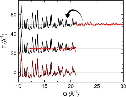
Figure 1: Demonstration of aliasing in $F(Q)$. (Top) Experimental nickel $F(Q)$ with $Q_{\mathrm{max}}=29.9~{}{\text{\AA}}^{-1}$ featuring regions above and below $Q^{\prime}=20.9~{}{\text{\AA}}^{-1}$. (Center) Experimental nickel $F(Q)$ with the region above $Q^{\prime}$ “folded” over to lower $Q$. (Bottom) Aliased $F(Q)$ obtained by sampling the PDF from the experimental $F(Q)$ on a grid with interval $dr=0.15~{}{\text{\AA}}$ and Fourier transforming back to $F(Q)$ (solid line). This sampling interval is larger than the Nyquist interval ($dr_{N}=0.105~{}{\text{\AA}}$) and corresponds to $Q^{\prime}=\pi/dr=20.9~{}{\text{\AA}}^{-1}$. Overlaid is the $F(Q)$ obtained by adding the unfolded and folded segments of the experimental $F(Q)$ (dashed line). Note that the $Q$-axis starts at $10~{}{\text{\AA}}^{-1}$.

We note that the case where the data are sampled precisely on a grid with the Nyquist interval, $dr=dr_{N}$, then $Q^{\prime}=Q_{m}=Q_{\mathrm{max}}$ and there is no folding. However, there is still loss of information since $\sin(Q_{m}ndr)=0$, and so the $m^{th}$ Fourier amplitude, $b_{m}$, can take on any value. This is why a strict inequality between the sampling interval and the Nyquist interval is required to avoid aliasing: $dr<dr_{N}$.

Aliasing implies that the sampled signal does not uniquely identify its source. Since some frequency components alias others, the PDF could represent the aliased $F(Q)$ just as well as the unaliased one. When back-Fourier transforming a sparsely sampled $G(r)$ into $Q$ space, the aliased $F(Q)$ will result. The sampling theorem states that aliasing does not occur when sampling at an interval smaller than the Nyquist interval.

3.2 Structural Information in the PDF

The sampling theorem determines the number of data points required to reconstruct a PDF signal from samples, which is

$$N=\Delta r/dr_{N}=\frac{\Delta rQ_{\mathrm{max}}}{\pi},$$ (5)

where $\Delta r$ is the extent of the PDF in $r$-space. What is more relevant to PDF modeling is the amount of structural information in the PDF. $N$ is an upper bound on this since we cannot extract more independent observations of the structure than raw information from the signal. Given perfect data and the proper model, one can meaningfully extract $N$ structural parameters from a PDF signal.

Factors such as noise and peak overlap can obscure the structural information in the PDF and therefore determine whether $N$ is a good estimate of the amount of structural information in the PDF. For example, consider a situation where the PDF contains a single peak, but has a very large $Q_{\mathrm{max}}$. In this case, a complete crystal model cannot be obtained from fitting this single peak, no matter how large $N$ is. In another extreme case, imagine that the majority of PDF peaks have a single point or no points due to a small $Q_{\mathrm{max}}$. In this situation the anisotropic displacement parameters cannot be determined with certainty.

In practice, the amount of structural information in the PDF cannot be precisely known. To perform a reliable refinement, the signal-to-noise ratio must be favorable, [10] the PDF peaks must be apparent, and the fit range must be such that the structural features one is seeking to model are accessible. In addition to this, we recommend using Rietveld refinement guidelines when refining the PDF, which advise that the ratio of independent observations to the number of refinement parameters should be around three to five, preferring the latter. [19]

4 Method

Powder diffraction data were collected from nickel and LaMnO₃ (LMO) samples. The nickel data were collected using the rapid acquisition pair distribution function (RaPDF) technique [20] with synchrotron x-rays on beamline 6-ID-D at the Advanced Photon Source at Argonne National Laboratory. The sample was purchased from Alfa Aesar. The powdered sample was packed in a flat plate holder with thickness of 1.0 mm and sealed between Kapton tapes. Data were collected at room temperature in transmission geometry with an x-ray energy of 98.001 keV ($\lambda=0.12651~{}{\text{\AA}}$). An image plate camera (Mar345) with diameter of 345 mm was mounted orthogonally to the beam with a sample to detector distance of 178.4 mm.

The raw 2D data were reduced to 1D integrated intensity profiles using the Fit2D program. [21] Corrections for environmental scattering, incoherent and multiple scattering, polarization and absorption were performed according to the standard procedures [10] using PDFgetX2 [5] to obtain the PDF with $Q_{\mathrm{max}}=29.9~{}{\text{\AA}}^{-1}$. This corresponds to $dr_{N}=0.105~{}{\text{\AA}}$.

The LMO data were collected using time-of-flight neutron diffraction at the NPDF instrument at the Los Alamos Neutron Scattering Center at Los Alamos National Laboratory. The LMO sample preparation and data collection have been described in detail elsewhere. [22] The LMO PDFs were produced with PDFgetN [7] using $Q_{\mathrm{max}}=32.0~{}{\text{\AA}}^{-1}$. This corresponds to $dr_{N}=0.0982~{}{\text{\AA}}$.

In each case, experimental PDFs were generated with $r_{\mathrm{max}}=20~{}{\text{\AA}}$ using $dr=0.01~{}{\text{\AA}}$. PDF data on sparser grids were created by removing points from this PDF in order to get the desired sampling interval. Pruning the data in this way is equivalent to recalculating the PDF from $F(Q)$ on the sparser grid. We produced 31 data-sets with varying $dr$ against which models were refined.

We took as a reference data-set the PDF generated on the default grid of $dr=0.01~{}{\text{\AA}}$ and structural models were refined to the data. We then refined the same models to data-sets on sparser grids. We define as $\Delta_{p}(dr)$ for a parameter $p$ as the absolute difference between the value of the parameter $p$ refined for the data-set sampled at interval $dr$ and that refined for the reference data-set. The accuracy of the refined parameters becomes unacceptable when $\Delta_{p}(dr)$ exceeds the statistical uncertainty on the difference, $\sigma(\Delta_{p}(dr))$. This is given by $\sigma(\Delta_{p}(dr))=\sqrt{\sigma^{2}(p(dr))+\sigma^{2}(p(0.01))}$, where $\sigma(p(dr))$ and $\sigma(p(0.01))$ are the estimated uncertainties on parameter $p$ taken from the refinement for the data-set sampled at interval $dr$ and the reference data-set, respectively. To determine if a refined parameter extracted from a sparse data set is accurate, we define a parameter quality factor, $\mathcal{Q}_{p}(dr)=\Delta_{p}(dr)/\sigma(\Delta_{p}(dr))$. If $\mathcal{Q}_{p}(dr)$ is less than or equal to one, the parameter value refined from the data-set sampled at interval $dr$ is within the expected uncertainty of the best estimate and is considered accurate. If $\mathcal{Q}_{p}(i)$ is greater than one, the change in the parameter’s value is greater than the expected uncertainty, and the result is considered unreliable.

The parameter quality measure, $\mathcal{Q}_{p}(i)$, is biased due to a couple of assumptions. First, by comparing all results with the refinement of the undiluted data we assume that this refinement gives the best estimate for each parameter. The validity of this assumption is dependent on the systematic bias of the refinement results due to the quality of the data and the suitability of the refinement model. Since this bias is present in the diluted data as well, its effects should be negligible. Second, we assume that the uncertainty value derived from the refinement results is accurate. We discuss later that the uncertainty values derived from refinements of oversampled data-sets are too small. This inflates the estimated quality factor when the data are oversampled, but does not invalidate the accompanying results.

The refinements from unaltered and sampled data-sets were performed identically over a range from $r_{\mathrm{min}}=0.01~{}{\text{\AA}}$ to $r_{\mathrm{max}}=20.0~{}{\text{\AA}}$ using the program PDFgui. [4] For the nickel data, the lattice parameter, isotropic atomic displacement parameter (ADP), dynamic correlation factor, scale factor and resolution factor were varied in the refinements. In the LMO fits, three lattice parameters, four isotropic ADPs (one each for the La, Mn and axial and planar oxygen atoms), and seven fractional coordinates were varied along with the scale and correlation factors (see [23]). From Eq. 5 we get that refinements over this range, $\Delta r=19.99~{}{\text{\AA}}$, yield $N_{Ni}=191$ and $N_{LMO}=203$. For the nickel data set, we have an observation-to-parameter ratio (OPR) greater than 30 and for LMO the OPR is greater than 10. The refinements are therefore comfortably over-constrained and the optimization problem is well conditioned.

Various refinements were timed to measure the speed-up in the program execution due to sampling.

5 Results

When the nickel and LMO data are made sparser, the PDF profiles appear less smooth and the detailed shape of the peak profiles becomes less apparent. This is shown in Figs. 2 and 3. The data in panel (a) in both figures are on the reference grid ($dr=0.01~{}{\text{\AA}}$) and are both smooth and have well-defined Gaussian-like peaks. [10] The data in panel (b) are sampled with $dr=0.1~{}{\text{\AA}}$, close to the Nyquist interval, and are not nearly as smooth, though the peaks are still well defined. Lastly, the data in panel (c) are sampled with $dr=0.3~{}{\text{\AA}}$, where there is apparent loss of information. The refined parameters from these fits are given in Table 1 and Table 2. Note that the uncertainty in the refined parameters increases from $dr=0.01~{}{\text{\AA}}$ to $dr=0.1~{}{\text{\AA}}$, although each of these data-sets produce acceptable results.

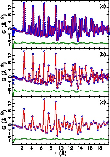
Figure 2: Fits to sampled nickel PDFs. (a) Unaltered data with $dr=0.01~{}{\text{\AA}}$. (b) Sampled data with $dr=0.1~{}{\text{\AA}}$. (c) Sampled data with $dr=0.3~{}{\text{\AA}}$. The data are shown as circles, the fits are the lines through the data and the difference is shown offset below. All fits are of similar quality, despite the poor visual quality of the data in panels (b) and (c). The data shown in panel (c) is undersampled and produced unacceptably uncertain results, though this is not apparent from the difference curve.

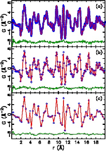
Figure 3: Fits to sampled LaMnO₃ PDFs. (a) Unaltered data with $dr=0.01~{}{\text{\AA}}$. (b) Sampled data with $dr=0.1~{}{\text{\AA}}$. (c) Sampled data with $dr=0.3~{}{\text{\AA}}$. The data are shown as circles, the fits are the lines through the data and the difference is shown offset below. All fits are of similar quality, despite the poor visual quality of the data in panels (b) and (c). The data shown in panel (b) and (c) are undersampled, and the data in panel (c) produced unacceptably uncertain results. Note that in panel (c) several peaks are not resolved.

Table 1: Parameters from Ni refinements using data with various $dr$. The Nyquist interval, $dr_{N}$, is $0.105~{}{\text{\AA}}$. Here, $a$ denotes the lattice parameter, $U_{iso}$ the isotropic ADP, $\delta_{2}$ the vibrational correlation parameter, $scale$ the data scale and $Q_{damp}$ the experimental resolution factor.

$dr({\text{\AA}})$	$0.01$	$0.10$	$0.12$	$0.30$
$a({\text{\AA}})$	3.53159(2)	3.53158(6)	3.53158(6)	3.53186(10)
$U_{iso}({\text{\AA}}^{2})$	0.005446(7)	0.00545(2)	0.00543(2)	0.00570(4)
$\delta_{2}({\text{\AA}}^{2})$	2.25(2)	2.20(5)	2.15(5)	2.2(2)
$scale$	0.7324(7)	0.733(2)	0.734(3)	0.761(4)
$Q_{damp}({\text{\AA}}^{-1})$	0.06307(11)	0.0632(4)	0.0634(4)	0.0653(7)

Table 2: Parameters from LaMnO₃ refinements using data with various $dr$. The Nyquist interval, $dr_{N}$, is $0.0982~{}{\text{\AA}}$. Here, $a$, $b$ and $c$ denote the lattice parameters, $U_{iso}$ the isotropic ADP (one for each primitive atom), $x$, $y$ and $z$ the fractional atomic coordinates, $\delta_{2}$ the vibrational correlation parameter and $scale$ the data scale.

$dr({\text{\AA}})$	$0.01$	$0.10$	$0.12$	$0.30$
$a({\text{\AA}})$	5.5394(2)	5.5394(6)	5.5393(7)	5.5362(14)
$b({\text{\AA}})$	5.7441(2)	5.7443(7)	5.7442(8)	5.7536(13)
$c({\text{\AA}})$	7.7059(2)	7.7059(9)	7.7054(10)	7.697(2)
$\delta_{2}({\text{\AA}}^{2})$	2.44(3)	2.38(9)	2.35(9)	2.49(14)
$scale$	0.7941(11)	0.794(3)	0.795(4)	0.803(6)
La
$x$	0.99234(10)	0.9923(3)	0.9926(4)	0.9917(6)
$y$	0.04828(8)	0.0482(2)	0.0481(3)	0.0469(5)
$U_{iso}({\text{\AA}}^{2})$	0.00508(4)	0.00506(13)	0.0052(2)	0.0055(2)
Mn
$U_{iso}({\text{\AA}}^{2})$	0.00376(7)	0.0038(2)	0.0038(2)	0.0024(3)
O1
$x$	0.07300(11)	0.0730(4)	0.0730(4)	0.0739(7)
$y$	0.48625(10)	0.4862(3)	0.4864(4)	0.4874(7)
$U_{iso}({\text{\AA}}^{2})$	0.00682(8)	0.0067(3)	0.0068(3)	0.0075(3)
O2
$x$	0.72515(8)	0.7251(2)	0.7252(3)	0.7247(5)
$y$	0.30682(8)	0.3068(3)	0.3069(3)	0.3072(5)
$z$	0.03876(6)	0.0388(2)	0.0389(2)	0.0399(3)
$U_{iso}({\text{\AA}}^{2})$	0.00689(4)	0.0069(2)	0.0068(2)	0.0062(2)

In Fig. 4 we show the parameter quality values, $\mathcal{Q}_{p}(i)$, plotted against the sampling interval. The quality factor is satisfactory for data-sets that are sampled with grids close to the reference data-set. This indicates that these refinements are producing the same parameter values. Near the Nyquist interval (indicated by the vertical dashed line), various quality factors become unacceptable.

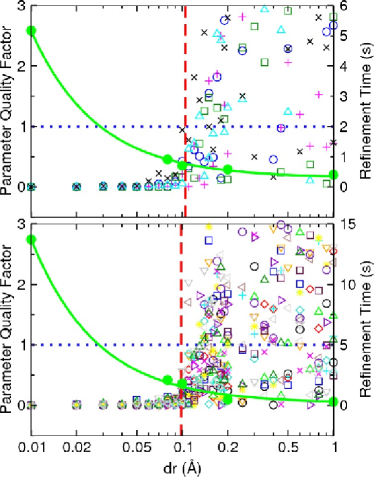
Figure 4: Refined parameter quality (open symbols) and refinement times (solid circles) measured using sampled Ni (top) and LaMnO₃ (bottom) data. The dotted horizontal line shows the cutoff between acceptable and unacceptable parameter quality. The dashed vertical line shows the value of $dr_{N}$ predicted by the sampling theorem. For $dr$ values larger than this the quality of some parameters transition into the unacceptable region. The time values demonstrate the decrease in refinement time with increasing $dr$, with more than a seven-fold speed up near $dr_{N}$. The solid curve through the time values is fit to the form $a+b/dr$.

6 Discussion

Figure 4 indicates that the onset of unreliable refinements coincides with the Nyquist interval. The refined parameter values are all acceptable, and largely independent of the sampling interval in the oversampling region ($dr<dr_{N}$). Figures 2, 3 and 4 indicate that visual appearance is not a good indicator of data quality.

The sampling theorem tells us that the information content in the data does not change as long as we sample on a grid finer than the Nyquist interval. We expect to and do refine the same parameters from such samples. As the data are sampled onto grids coarser than the Nyquist interval, we expect to lose structural information gradually. In contrast, refined values of the parameters become unreliable quickly as the Nyquist interval is exceeded. This is somewhat surprising since the refinements are highly overconstrained and have an estimated OPR greater than 5 even when sampled at twice the Nyquist interval. In Fig. 4 we see the quality of the refined parameters diverge well before this point. Intuition would tell us that it is possible to lose a considerable quantity of information by sampling before refinements become unstable. This is not observed. The instability is not caused solely by information loss, but by information corruption due to aliasing.

Aliasing has two effects on a PDF signal, as described in Section 3.1. Foremost, aliasing lowers the effective maximum $Q$-value in $F(Q)$ from $Q_{\mathrm{max}}$ to $Q^{\prime}=\pi/dr$. This creates the obvious effect of lower resolution in the PDF, as seen in Figs. 2 and 3. In extreme cases, this will lead to poorly defined peaks in the PDF. Less obviously, sampling on a grid coarser than the Nyquist interval allows for the possibility that the PDF has originated from a different, aliased, $F(Q)$ as shown in Fig. 1. When calculating the model PDF, we enforce $F(Q>Q_{\mathrm{max}})=0$. When there is aliasing the structure function resulting from $G(r)$ has $F(Q>\pi/dr=0)$, and extra intensity below $\pi/dr$. Thus, aliasing makes it possible to find a different set of refinement parameters that describes the sampled PDF. This is true regardless of the optimization algorithm.

The estimated uncertainties on the fitting parameters for $dr$ in the region of stable refinements are dependent on the sampling interval. We see from Tables 1 and 2 that the uncertainties on the parameters increase when estimated from the data sampled near the Nyquist interval compared to the reference data. The sampling theorem gives the number of data points necessary to fully represent the PDF. Any data sampled on a grid finer than the Nyquist interval are necessarily redundant. If a set of fitting parameters reproduces a particular set of points well on a optimal grid, those parameters will also reproduce the associated redundant points well. By not taking into account the correlations between data points, [9] as in this study, this results in under-estimated uncertainty values on parameters. Refining optimally sampled data reduces these correlations while retaining all the structural information available in the data and gives a more reliable estimate of uncertainties.

A fortunate side-effect of refining optimally sampled data is a decreased refinement time. Shown in Fig. 4 is a plot of refinement times for some chosen sampling intervals. The trend in the plot shows that refinement time is proportional to the inverse of $dr$ (shown as the broad solid line), or directly proportional to the number of data points, with a constant offset. This trend reflects the fact that the calculation of the PDF grows linearly with the number of sample points. Carrying out refinements on optimally sampled data gives a significant speed increase compared to the reference data; in this case the speed increases by more than a factor of seven.

These observations indicate that PDF refinements should be performed on the sparsest grid possible with sampling interval less than the Nyquist interval. To produce an esthetically pleasing presentation of the PDF, one can interpolate onto a finer grid using the Whittaker-Shannon interpolation formula (Eq. 4).

7 Conclusions

The purpose of this research was to demonstrate the consequences of the Nyquist-Shannon sampling theorem as it applies to the PDF. We show that the quality of refined parameters diverges when sampling the PDF at intervals larger than the Nyquist interval, which is the result of aliasing. Furthermore, we show that the estimated uncertainties of refined parameters are more reliable when the PDF is optimally sampled. Statistically reliable uncertainties on refined parameters can be obtained by taking into account the correlations between all the points in $G(r)$, [9] but this comes at the computational expense of inverting a large error matrix. By optimally sampling the PDF, the correlations among points in the PDF are minimized while preserving all the available structural information. This gives improved uncertainty estimates without costly computation, and may expedite refinements when the PDF can be computed over fewer points.

The Nyquist-Shannon sampling theorem gives an upper bound on the amount of structural information contained in an experimental PDF. This determines the $Q$- and $r$-extent that are required for a model refinement to be overconstrained. Oversampling the PDF does not add more information to a refinement, and therefore provides no benefit other than an esthetically pleasing visualization. This result emphasizes the importance of collecting diffraction data to high $Q$ when it is to be used for PDF modeling, since a larger $Q_{\mathrm{max}}$ decreases the Nyquist interval, and makes accessible smaller structural details.

8 Acknowledgments

M. S. would like to thank the entire Billinge-group lab for helping and supporting her throughout this summer project - Jiwu, Pavol, Ahmad, and especially Hyun-Jeong. Lastly, she thanks Dr. Richmond at Michigan State University for putting together an amazing summer high-school research experience program. Research in the Billinge group was supported by the US National Science foundation through Grant DMR-0703940. Use of the APS is supported by the U.S. DOE, Office of Science, Office of Basic Energy Sciences, under Contract No. W-31-109-Eng-38. The 6ID-D beamline in the MUCAT sector at the APS is supported by the U.S. DOE, Office of Science, Office of Basic Energy Sciences, through the Ames Laboratory under Contract No. W-7405-Eng-82. Beamtime on NPDF at Lujan Center at Los Alamos National Laboratory was funded under DOE Contract No. DEAC52-06NA25396.

References

- [1] Billinge, S. J. L. and Levin, I. (2007) Science 316, 561–565.
- [2] Proffen, T., Egami, T., Billinge, S. J. L., Cheetham, A. K., Louca, D., and Parise, J. B. (2002) Appl. Phys. A 74, s163–s165.
- [3] Chupas, P. J., Chapman, K. W., and Lee, P. L. (2007) J. Appl. Crystallogr. 40, 463–470.
- [4] Farrow, C. L., Juhás, P., Liu, J., Bryndin, D., Božin, E. S., Bloch, J., Proffen, T., and Billinge, S. J. L. (2007) J. Phys: Condens. Mat. 19, 335219.
- [5] Qiu, X., Thompson, J. W., and Billinge, S. J. L. (2004) J. Appl. Crystallogr. 37, 678.
- [6] Tucker, M. G., Dove, M. T., and Keen, D. A. (2001) J. Appl. Crystallogr. 34, 630–638.
- [7] Peterson, P. F., Gutmann, M., Proffen, T., and Billinge, S. J. L. (2000) J. Appl. Crystallogr. 33, 1192–1192.
- [8] Proffen, T. and Billinge, S. J. L. (1999) J. Appl. Crystallogr. 32, 572–575.
- [9] Toby, B. H. and Billinge, S. J. L. (2004) Acta Crystallogr. A 60, 315–317.
- [10] Egami, T. and Billinge, S. J. L. (2003) Underneath the Bragg peaks: structural analysis of complex materials, Pergamon Press, Elsevier, Oxford, England.
- [11] Schwarzenbach, D., Abrahams, S. C., Flack, H. D., Gonschorek, W., Th. Hahn, Huml, K., Marsh, R. E., Prince, E., Robertson, B. E., Rollett, J. S., and Wilson, A. J. C. (1989) Acta Crystallogr. A 45, 63–75.
- [12] Shannon, C. E. (1949) Proc. IRE 37, 10–21.
- [13] Billinge, S. J. L. (2008) J. Solid State Chem. 181, 1698–1703.
- [14] Billinge, S. J. L. and Kanatzidis, M. G. (2004) Chem. Commun. 2004, 749–760.
- [15] Farrow, C. L. and Billinge, S. J. L. (2009) Acta Crystallogr. A 65(3), 232–239.
- [16] Levenberg, K. (1944) Q. Appl. Math 2, 164–168.
- [17] Marquardt, D. (1963) SIAM J. Appl. Math 11, 431–441.
- [18] Whittaker, E. (1915) Proc. R. Soc. Edinb. A 35, 181–194.
- [19] McCusker, L. B., Dreele, R. B. V., Cox, D. E., Louër, D., and Scardi, P. (1999) J. Appl. Crystallogr. 32, 36.
- [20] Chupas, P. J., Qiu, X., Hanson, J. C., Lee, P. L., Grey, C. P., and Billinge, S. J. L. (2003) J. Appl. Crystallogr. 36, 1342–1347.
- [21] Hammersley, A. P. Fit2d v9.129 reference manual v3.1 ESRF Internal Report ESRF98HA01T (1998).
- [22] Qiu, X., Th. Proffen, Mitchell, J. F., and Billinge, S. J. L. (2005) Phys. Rev. Lett. 94, 177203.
- [23] Božin, E. S., Qiu, X., Schmidt, M., Paglia, G., Mitchell, J. F., Radaelli, P. G., Proffen, T., and Billinge, S. J. L. (2006) Physica B 385-386, 110–112.