Primordial Non-Gaussianity and the Statistics of Weak Lensing and other Projected Density Fields

Abstract

Estimators for weak lensing observables such as shear and convergence generally have non-linear corrections, which, in principle, make weak lensing power spectra sensitive to primordial non-Gaussianity. In this paper, we quantitatively evaluate these contributions for weak lensing auto- and cross-correlation power spectra, and show that they are strongly suppressed by projection effects. This is a consequence of the central limit theorem, which suppresses departures from Gaussianity when the projection reaches over several correlation lengths of the density field, $L_{P}\sim 55\,{\rm Mpc}/h$. Furthermore, the typical scales that contribute to projected bispectra are generally smaller than those that contribute to projected power spectra. Both of these effects are not specific to lensing, and thus affect the statistics of non-linear tracers (e.g., peaks) of any projected density field. Thus, the clustering of biased tracers of the three-dimensional density field is generically more sensitive to non-Gaussianity than observables constructed from projected density fields.

I Introduction

In recent years, a renewed interest in the effects of primordial non-Gaussianity on the large-scale structure of the Universe has emerged, prompted by the significant effect on the bias of dark matter halos at large scales measured in N-body simulations Dalal et al. (2008); Desjacques et al. (2009); Grossi et al. (2009); Pillepich et al. (2010); Wagner and Verde (2011); Desjacques et al. (2011a). The observation of this effect in redshift surveys would be able to provide an independent confirmation of a possible detection of primordial non-Gaussianity from the anisotropies of the cosmic microwave background (CMB). Such a detection would open a completely new perspective on inflation and the high-energy physics of the early Universe (see, for instance, Komatsu et al., 2009a).

In fact, a specific type of non-Gaussian initial conditions, i.e. the local model of primordial non-Gaussianity (Salopek and Bond, 1990; Komatsu and Spergel, 2001), induces a strongly scale-dependent correction to the linear halo bias. This correction has been derived using several approaches, mostly based on the peak-background split formalism (Dalal et al., 2008; Slosar et al., 2008; Afshordi and Tolley, 2008; Desjacques et al., 2009; Giannantonio and Porciani, 2010; Schmidt and Kamionkowski, 2010) or on the statistics of high-peaks (Matarrese et al., 1986; Matarrese and Verde, 2008) (also, see (McDonald, 2008) for a different perspective). On the other hand, one can make the simple assumption of a local but nonlinear bias relation between the galaxy distribution and the underlying matter field Scoccimarro (2000). When applied to the local model of non-Gaussianity, this yields the same scale-dependent correction as obtained in the former two approaches Taruya et al. (2008); Desjacques et al. (2011b).

The effect due to nonlinear local biasing shows an especially close analogy with the case of non-linear weak lensing estimators we consider in this paper. A nonlinear but local galaxy bias relation can be expressed by the Taylor expansion (Fry and Gaztañaga, 1993)

$$\delta_{g}(x)=b_{1}\,\delta(x)+\frac{1}{2}b_{2}\,\delta^{2}(x)+\cdots\,,$$ (1)

where $\delta_{g}(x)$ and $\delta(x)$ represent, respectively, the galaxy and matter density contrasts and $b_{1}$ and $b_{2}$ are the linear and quadratic bias parameters, which are assumed to be constants for a given galaxy sample. This leads to the following perturbative expansion for the galaxy two-point correlation function:

$$\langle\delta_{g}(x_{1})\delta_{g}(x_{2})\rangle=\> b_{1}^{2}\langle\delta(x_{1})\delta(x_{2})\rangle$$

$$+\frac{1}{2}b_{1}b_{2}\left[\langle\delta(x_{1})\delta^{2}(x_{2})\rangle+(x_{1}\leftrightarrow x_{2})\right]$$

$$+\cdots\,,$$ (2)

where the second term on the r.h.s. depends on the matter 3-point correlation function or bispectrum. For Gaussian initial conditions, the matter bispectrum induced by gravitational instability leads to negligible corrections in the two-point correlation on large scales. For non-Gaussian initial conditions of the local type, on the other hand, the correction becomes relevant on large scales.

Since such behavior arises simply from the nonlinear relation between the observed distribution $\delta_{g}$ and the matter distribution $\delta$, we expect similar effects to show up for any other large-scale structure observables where analogous nonlinearities are present.

Weak lensing measures the three components $\kappa$, $\gamma_{1}$, $\gamma_{2}$ of the tidal tensor of the lensing potential $\psi$,

$$\psi_{,ij}=\> \left(\begin{array}[]{cc}\kappa+\gamma_{1}&\gamma_{2}\\ \gamma_{2}&\kappa-\gamma_{1}\end{array}\right)\,,$$ (5)

$$\psi(\bm{\theta})\equiv\> \int_{0}^{\chi_{s}}d\chi\>\frac{\chi_{s}-\chi}{\chi\chi_{s}}\>\Phi_{-}(\chi\bm{\theta};\chi)\,,$$ (6)

where derivatives are with respect to angular coordinates on the sky (we assume small angles, zero curvature, and a flat sky limit throughout), $\chi$ denotes comoving distance, while $\chi_{s}$ is the distance to the source galaxy being lensed, and $\Phi_{-}=(\Psi-\Phi)/2$ is the lensing potential in conformal Newtonian, or longitudinal, gauge.

While the two components of the shear $\gamma_{i}$ can be measured using galaxy ellipticities, the convergence $\kappa$ can be measured either through its effects on the number density of galaxies (magnification bias), or on galaxy sizes and fluxes. In all of these cases, the estimators are not purely linear. This is not surprising since Eq. (5) is only a lowest order approximation to the lensing effect. Given that the shear $\gamma$ is a (two-dimensional) spin-2 field while $\kappa$ is a scalar, we can generally write

$$\gamma^{\rm obs}(\bm{\theta})=\> \gamma(\bm{\theta})+c_{\gamma}\kappa(\bm{\theta})\gamma(\bm{\theta})+\cdots$$ (7)

$$\kappa^{\rm obs}(\bm{\theta})=\> \kappa(\bm{\theta})+c_{\kappa 1}\kappa^{2}(\bm{\theta})$$ (8)

$$+c_{\kappa 2}[\gamma_{1}^{2}(\bm{\theta})+\gamma_{2}^{2}(\bm{\theta})]+\cdots,$$

where $\kappa^{\rm obs},\gamma^{\rm obs}$ are the measured convergence and shear, and the dots indicate third- and higher order terms. For simplicity, we have assumed that all additive and multiplicative biases have been removed so that to lowest order, $\kappa^{\rm obs}=\kappa$ and $\gamma^{\rm obs}=\gamma$.

In the case of shear measurements from galaxy surveys, corrections to the leading order come from two sources: the fact that galaxy shapes estimate the reduced shear $g=\gamma/(1-\kappa)$ rather than the shear $\gamma$ (White, 2005; Dodelson et al., 2006a; Bernardeau et al., 2010); and lensing bias Schmidt et al. (2009a), the fact that we preferentially select lensed galaxies in a flux- and size-limited source galaxy sample. Following the estimate of Schmidt et al. (2009b), these two effects add up, yielding $c_{\gamma}$ roughly between $2$ and $3$.

Examples of measurements of the convergence include using the number density of background galaxies via the magnification and size bias effects (Broadhurst et al., 1995; Scranton et al., 2005), and using the sizes and other measured characteristics of galaxies (Jain, 2002; Bertin and Lombardi, 2006; Rozo and Schmidt, 2010). All these estimators in fact measure the magnification $\mu$,

$$\mu(\bm{\theta})=\frac{1}{(1-\kappa)^{2}-|\gamma|^{2}}=1+2\kappa+3\kappa^{2}+|\gamma|^{2}+\cdots$$ (9)

Hence, in the ideal case we expect $c_{\kappa 1}=3/2$ and $c_{\kappa 2}=1/2$. These values will likely be modified in practice due to galaxy selection effects similar to those present in the shear. Note that it is often possible to vary the non-linearity coefficients $c_{\gamma},c_{\kappa}$ experimentally, for example by applying different cuts on the source galaxy sample.

In analogy with Eq. (2), the two-point correlation of a non-linear estimator such as Eqs. (7)–(8) receives corrections from three- and higher point functions of the underlying density field. This is easy to see e.g. for the shear two-point function (neglecting the spinor indices for simplicity):

$$\langle\gamma^{\rm obs}(\bm{\theta})\gamma^{\rm obs}(\bm{\theta}^{\prime})\rangle=\> \langle\gamma(\bm{\theta})\gamma(\bm{\theta}^{\prime})\rangle$$

$$+2c_{\gamma}\langle\kappa(\bm{\theta})\gamma(\bm{\theta})\gamma(\bm{\theta}^{\prime})\rangle+\cdots$$ (10)

The leading correction term is a three-point function of shear and convergence, evaluated in the limit where two of the three vertices coincide. In Dodelson et al. (2006b); Shapiro (2009); Schmidt et al. (2009a), this contribution was investigated for non-Gaussianities from the non-linear evolution of the matter density. However, primordial non-Gaussianity also modifies the shear and convergence power spectra in the same way. Throughout this paper, we shall focus on the local model of non-Gaussianity, where the bispectrum of primordial curvature perturbations, evaluated at last scattering, is given by

$$B_{\phi}(k_{1},k_{2},k_{3})=2{f_{\rm{NL}}}[P_{\phi}(k_{1})P_{\phi}(k_{2})+{\rm perm.}].\vspace*{0.2cm}$$ (11)

Our conclusions however are broadly valid for any primordial bispectrum shape.

It will be useful to compare the impact of non-Gaussianity on weak lensing correlations with the analogous effects on the clustering of large-scale structure tracers such as galaxies or halos. As shown in Dalal et al. (2008), tracers with a linear (Eulerian) bias $b_{1}$ acquire a scale-dependent bias correction in the presence of local non-Gaussianity given by

$$\Delta b_{1}(k;z)=\frac{2{f_{\rm{NL}}}(b_{1}-1)\delta_{c}}{\mathcal{M}(k,z)},$$ (12)

where $\delta_{c}=1.686$ is the critical density for the spherical collapse in the flat matter dominated universe. The function $\mathcal{M}(k,z)$, which relates the matter density fluctuations to the initial curvature perturbations as $\delta(\mathbf{k})=\mathcal{M}(k,z)\phi(\mathbf{k})$, is given by

$$\mathcal{M}(k,z)\equiv\frac{k^{2}\>T(k)}{C_{P}}D(z).$$ (13)

where $T(k)$ is the matter transfer function, $C_{P}\equiv 3/2\>\Omega_{m}H_{0}^{2}$, and $D(z)$ is the linear growth function normalized to the scale factor at last scattering (at which in our convention $f_{\rm NL}$ is defined), that is $D(z_{ls})=1/(1+z_{ls})$.

Throughout this paper, we shall also assume the Limber approximation and work in the small angle limit, where the spherical harmonic transform is reduced to the two-dimensional Fourier transform. This very useful approximation does not significantly influence our results Jeong et al. (2009). We also assume that sources reside at a fixed redshift. Our fiducial cosmology is defined through the maximum likelihood cosmological parameters in Table 1 (“WMAP5+BAO+SN”) of Komatsu et al. (2009b).

We begin in Sec. II by studying the impact of non-Gaussianity on shear and convergence power spectra. We then investigate the cross-correlation of shear and convergence with large-scale structure (LSS) tracers in Sec. III. Sec. IV extends the arguments to the general case of the clustering of peaks (or more generally nonlinear tracers) identified in projected density fields. We conclude in Sec. V

II Shear and convergence power spectra

We first consider the impact of primordial non-Gaussianity on large-scale shear and convergence power spectra. By Fourier transforming Eq. (I) and the analogous equation for the convergence, we obtain the observed shear and convergence power spectra:

$$C_{\gamma^{\rm obs}}(\ell)=\> C_{\kappa}(\ell)+2c_{\gamma}\!\int\!\frac{d^{2}\ell_{1}}{(2\pi)^{2}}\cos 2\phi_{\ell_{1}}B_{\kappa}(\ell_{1},|\bm{\ell}-\bm{\ell}_{1}|,\ell)\,,$$ (14)

$$C_{\kappa^{\rm obs}}(\ell)=\> C_{\kappa}(\ell)+2\!\int\!\frac{d^{2}\ell_{1}}{(2\pi)^{2}}\left[c_{\kappa 1}+2c_{\kappa 2}\cos 2(\phi_{\ell_{1}}-\phi_{\ell-\ell_{1}})\right]B_{\kappa}(\ell_{1},|\bm{\ell}-\bm{\ell}_{1}|,\ell)\,.$$ (15)

Here, $B_{\kappa}$ is the convergence bispectrum, and we have aligned $\bm{\ell}_{1}$ so that $\phi_{\ell}=0$. Further, we have used that in Fourier space $\gamma(\bm{\ell})=\gamma_{1}(\bm{\ell})+i\gamma_{2}(\bm{\ell})=\exp(2i\phi_{\ell})\kappa(\bm{\ell})$, and hence the leading order shear power spectrum is equal to the leading order convergence power spectrum $C_{\kappa}(\ell)$. The convergence power spectrum and bispectrum are related to the corresponding matter correlators $P_{m},\;B_{m}$ via

$$C_{\kappa}(\ell)\! = \!C_{P}^{2}\!\int_{0}^{\chi_{s}}\frac{d\chi}{\chi}\frac{W_{L}^{2}(\chi_{s},\chi)}{\chi\>a^{2}(\chi)}P_{m}(\ell/\chi;\chi)\,,\ \ \ \$$ (16)

$$B_{\kappa}(\ell_{1},\ell_{2},\ell_{3})\! = \!C_{P}^{3}\!\int_{0}^{\chi_{s}}\frac{d\chi}{\chi}\frac{W_{L}^{3}(\chi_{s},\chi)}{\chi^{3}\>a^{3}(\chi)}$$ (17)

$$\qquad\times B_{m}\!\left(\frac{\ell_{1}}{\chi},\frac{\ell_{2}}{\chi},\frac{\ell_{3}}{\chi};\chi\right),$$

where $W_{L}(\chi_{s},\chi)\equiv\chi/\chi_{s}(\chi_{s}-\chi)$ denotes the lensing kernel.

In Eulerian Perturbation Theory (PT), the leading order expression (“tree-level”) of the matter bispectrum, valid at large scales, is given by the sum of a primordial component, $B_{I}$, present for non-Gaussian initial conditions, and a contribution $B_{G}$ due to second-order corrections to the matter density induced by gravitational instability. We have

$$B_{m}=B_{I}+B_{G}+...\,,$$ (18)

where the dots represent higher-order corrections in PT. The primordial component $B_{I}$ is directly related to the primordial curvature bispectrum $B_{\phi}$ via

$$B_{I}(k_{1},k_{2},k_{3};z)=\> \mathcal{M}(k_{1},z)\mathcal{M}(k_{2},z)\mathcal{M}(k_{3},z)$$

$$\times B_{\phi}(k_{1},k_{2},k_{3})\,,$$ (19)

while the non-linear component $B_{G}$ is given by

$$B_{G}(k_{1},k_{2},k_{3};z)=\> 2F_{2}(\mathbf{k}_{1},\mathbf{k}_{2})P_{L}(k_{1};z)P_{L}(k_{2};z)$$

$$+(2~{}{\rm perm.})\,,$$ (20)

where $P_{L}(k;z)=\mathcal{M}(k,z)^{2}P_{\phi}(k)$ is the linear matter power spectrum, and

$$F_{2}(\mathbf{k}_{1},\mathbf{k}_{2})=\> 5/7+(1/2)\mathbf{\hat{k}}_{1}\cdot\mathbf{\hat{k}}_{2}(k_{1}/k_{2}+k_{2}/k_{1})$$

$$+(2/7)(\mathbf{\hat{k}}_{1}\cdot\mathbf{\hat{k}}_{2})^{2}.$$ (21)

Note that at small scales, additional perturbative corrections become relevant and, in general, it is not possible to separate out the purely primordial components in the matter bispectrum (Sefusatti, 2009; Sefusatti et al., 2010). We shall return to this issue below.

From the non-Gaussianity viewpoint, Eqs. (14)–(15) come as no surprise: neglecting the distinction between $\gamma$ and $\kappa$ for the moment, Eqs. (7)–(8) say that the observed shear and convergence are biased estimates of the true $\gamma$, $\kappa$ with linear bias $b_{1}=1$ and quadratic bias parameters $b_{2}=c_{\gamma},c_{\kappa}$. Hence, Eqs. (14)–(15) are analogous to the expression for the non-Gaussian halo power spectrum Taruya et al. (2008), with two differences: first, we are dealing with the projected density field $\kappa$; second, the relation between shear and convergence leads to cosine factors in the integral. Note that on large scales, the bispectrum $B_{\kappa}$ is evaluated in the squeezed limit, since typically $\ell\ll\ell_{1}$. This is again similar to the halo clustering case.

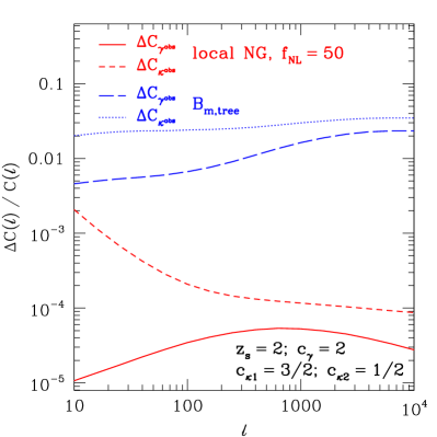
Figure 1: Relative correction to the shear and convergence power spectra from primordial NG of the local type (red solid/dashed), and the tree-level matter bispectrum from non-linear evolution (blue long-dashed/dotted). Here, we have assumed sources located at $z_{s}=2$ and non-linear parameters as indicated in the figure (see Sec. I).

Fig. 1 shows the relative amplitude of the correction to the shear and convergence power spectra from a numerical evaluation of Eqs. (14)–(15) when using the primordial bispectrum of the local type. We also show the tree-level bispectrum from non-linear evolution which contributes at the percent-level to $C_{\gamma^{\rm obs}}$ and $C_{\kappa^{\rm obs}}$. Clearly, the contributions from primordial non-Gaussianity are strongly suppressed: they are always below $10^{-4}$ for the shear, and only reach $10^{-3}$ at the very largest scales for the convergence. This is in stark contrast to the results for the halo power spectrum Dalal et al. (2008); Slosar et al. (2008) where order unity corrections are observed for this type of non-Gaussianity on large scales.

In order to understand where this suppression comes from, we make an order of magnitude estimate of Eqs. (14)–(15). We approximate the convergence power and bispectrum as

$$C_{\kappa}(\ell)\sim C_{P}^{2}\,\bar{\chi}\,x_{P}^{2}\,P_{L}(\ell/\bar{\chi};\bar{\chi})\,,$$ (22)

and

$$B_{\kappa}(\ell_{1},\ell_{2},\ell_{3})\sim C_{P}^{3}\,x_{B}^{3}\,B_{I}\left(\frac{\ell_{1}}{\bar{\chi}},\frac{\ell_{2}}{\bar{\chi}},\frac{\ell_{3}}{\bar{\chi}};\bar{\chi}\right)\,.$$ (23)

Here, $\bar{\chi}$ is an effective lens distance, and $x_{P}$, $x_{B}$ are dimensionless geometrical factors of order unity which we leave unspecified for the moment. On large scales, the bispectrum is evaluated in the squeezed limit, $k_{1}\gg k$. In the squeezed limit, Eq. (11) asymptotes approximately to

$$B_{I}(k_{1},k,|\mathbf{k}_{1}\!-\!\mathbf{k}|)\> =2\,f_{\rm NL}\,\mathcal{M}(k)\mathcal{M}(k_{1})\mathcal{M}(|\mathbf{k}_{1}\!-\!\mathbf{k}|)$$

$$\quad\times P_{\phi}(k)\left[P_{\phi}(k_{1})\!+\!P_{\phi}(|\mathbf{k}_{1}\!-\!\mathbf{k}|)\right]\ \$$ (24)

$$\sim 4\,f_{\rm NL}\,\mathcal{M}(k)P_{\phi}(k)P_{L}(k_{1})$$ (25)

neglecting the third permutation which is suppressed. In the second approximate equality, we also set $|\mathbf{k}_{1}-\mathbf{k}|\approx k_{1}$. Further, for the moment all power spectra are assumed to be evaluated at $z(\bar{\chi})$. After some manipulation, we arrive at the following estimates:

$$\Delta C_{\gamma^{\rm obs}}(\ell)\approx\> 0\,,$$ (26)

$$\Delta C_{\kappa^{\rm obs}}(\ell)\approx\> 8f_{\rm NL}\frac{(c_{\kappa 1}+c_{\kappa 2})\sigma_{\kappa}^{2}}{C_{P}\bar{\chi}^{2}x_{B}}\left(\frac{x_{B}}{x_{P}}\right)^{2}$$

$$\times\mathcal{M}^{-1}(\ell/\bar{\chi})C_{\kappa}(\ell)\,,$$ (27)

where

$$\sigma_{\kappa}^{2}=\int\frac{d^{2}\ell}{(2\pi)^{2}}C_{\kappa}(\ell).$$ (28)

The $\cos 2\phi_{\ell_{1}}$ factor in Eq. (14) leads to a complete cancelation of the effect on $C_{\gamma^{\rm obs}}$ in this approximation, while the phase factor in the second term of Eq. (15) becomes unity. Further, note that in reality there is a high$-\ell$ cut-off in Eq. (28) due to the resolution or pixel size of the shear survey. As long as this cut-off is less than $\sim$ arcmin-scale, however, the quantitative results do not depend sensitively on the resolution.

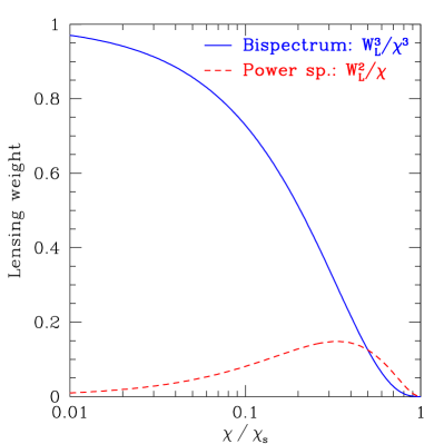
Figure 2: Effective lensing weight functions for the shear power spectrum (red dashed), and the shear bispectrum (blue solid).

Using Eq. (22), Eq. (27) can be further simplified to yield

$$\frac{\Delta C_{\kappa^{\rm obs}}(\ell)}{C_{\kappa}(\ell)}\approx 8f_{\rm NL}\frac{c_{\kappa}}{\ell^{2}T(\ell/\bar{\chi})}\frac{\sigma_{\kappa}^{2}}{x_{B}}\left(\frac{x_{B}}{x_{P}}\right)^{4},$$ (29)

where $c_{\kappa}=c_{\kappa 1}+c_{\kappa 2}$. Note the appearance of an $\ell^{-2}$, just as a factor of $k^{-2}$ appears in the halo biasing in the local model of NG Dalal et al. (2008). In fact, it is instructive to compare Eq. (29) to a similar estimate for the angular power spectrum of some biased tracer “$h$”. Using the Limber approximation, we have

$$C_{hh}(\ell)=\int\frac{d\chi}{\chi}\frac{F_{h}(\chi)^{2}}{\chi}P_{hh}\left(\frac{\ell}{\chi};\chi\right),$$ (30)

where $F_{h}(\chi)$ is the selection function, normalized to unity in comoving distance. Let us now assume that the tracer is localized in a narrow redshift slice around a comoving distance $\bar{\chi}$. Given that $P_{hh}(k)=[b_{1}+\Delta b(k)]^{2}P_{m}(k)$ where $\Delta b$ is given by Eq. (12) in the local model of NG, we can approximately write the leading correction to $C_{hh}$ as

$$\frac{\Delta C_{hh}(\ell)}{C_{hh}(\ell)}\approx 2{f_{\rm{NL}}}\frac{b_{1}-1}{b_{1}}\delta_{c}\frac{C_{P}\bar{\chi}^{2}}{D(\bar{z})\,\ell^{2}T(\ell/\bar{\chi})},$$ (31)

where $\bar{z}=z(\bar{\chi})$. Assuming that $\bar{\chi}$ is a cosmological distance, all factors in Eq. (31) are in fact of order unity. Comparing Eq. (31) with Eq. (29) shows that the suppression of the impact of non-Gaussianity on weak lensing power spectra comes from two sources: first, it is suppressed by $\sigma_{\kappa}^{2}\sim 10^{-3}$. As we will show in Sec. IV, this suppression factor is due to the projection of the density field over many correlation lengths, and thus ultimately a consequence of the central limit theorem. Second, the projection kernel for the bispectrum strongly prefers small lens distances, so that $x_{B}\ll x_{P}\sim 0.5$. To illustrate this, Fig. 2 shows the redshift weighting function of the shear bispectrum and power spectrum in comparison. Clearly, most of the contribution to the shear bispectrum comes from low redshifts, $\chi/\chi_{s}\lesssim 0.2$. In other words, for a survey with $z_{s}=2$ ($\chi_{s}\sim 3700\,{\rm Mpc}/h$), the shear bispectrum hardly probes scales above $700\,{\rm Mpc}/h$. Since the effect (at least from local NG) peaks on large scales, this is a severe limitation.

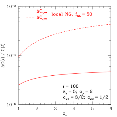
Figure 3: Relative amplitude of the non-linear lensing correction from primordial non-Gaussianity to the shear and convergence power spectra as function of the source redshift $z_{s}$, for a fixed multipole $\ell=100$. The other parameters are at the same values as for Fig. 1.

Finally, choosing some numbers, $\sigma_{\kappa}^{2}=10^{-3}$, $x_{B}=0.2$, $x_{P}=0.5$, and setting $T=1$, we have

$$\frac{\Delta C_{\kappa^{\rm obs}}(\ell)}{C_{\kappa}(\ell)}\sim 10^{-4}\left(\frac{f_{\rm NL}}{100}\right)\left(\frac{\ell}{100}\right)^{-2}.$$ (32)

Comparing with Fig. 1, we see that the order-of-magnitude estimate predicts the right amplitude to within a factor of a few. We also see the $\ell^{-2}$ behavior for $\Delta C_{\kappa^{\rm obs}}$ on large scales, and that $\Delta C_{\gamma^{\rm obs}}$ is indeed strongly suppressed for small $\ell$ due to the cosine factor in Eq. (14). The restriction to small scales due to the lensing projection can be somewhat mitigated by going to larger source redshifts. Fig. 3 shows the evolution of the non-linear corrections with source redshift. While the corrections, especially $\Delta C_{\kappa^{\rm obs}}$, increase with $z_{s}$, the corrections remain much smaller than $10^{-3}$ at $\ell=100$.

II.1 Impact of non-linearities on small scales

So far, we have only considered the leading order (tree-level) contribution to the matter bispectrum from primordial non-Gaussianity. A simple estimate of the effect of non-linearities can be obtained directly from Eq. (29), by replacing $\sigma_{\kappa}^{2}$ with the non-linear variance of the convergence. Since $\sigma_{\kappa,\rm NL}^{2}\sim 5\sigma_{\kappa}^{2}$ (estimated using the non-linear matter power spectrum from halofit Smith et al. (2003)), non-linearities are expected to increase $\Delta C_{\kappa}^{\rm obs}(\ell)$ by the same factor. We can obtain a somewhat more sophisticated estimate by using the fact that, in the local model of non-Gaussianity, a long wavelength (linear) perturbation $\phi_{l}$ acts to increase the variance of small-wavelength matter perturbations $\delta_{L,s}$ Dalal et al. (2008); Slosar et al. (2008):

$$\langle\delta_{L,s}^{2}\rangle\rightarrow\langle\delta_{L,s}^{2}\rangle\>(1+4f_{\rm NL}\phi_{l})\,,$$ (33)

where all perturbations here are evaluated at early times, i.e. in Lagrangian space (indicated by subscript “$L$”). This is clearly reflected in the approximate squeezed-limit expression for $B_{m}$, Eq. (25) (since $\mathcal{M}(k)P_{\phi}(k)=\langle\delta_{l}\phi_{l}\rangle$).

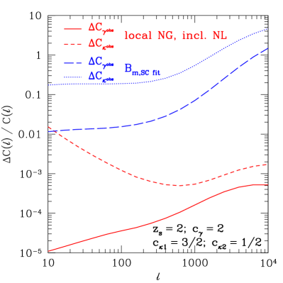
Figure 4: Same as Fig. 1, but with non-linear corrections included. For the corrections from primordial non-Gaussianity (red solid/dashed), we use the matter bispectrum from Eq. (35) with $P_{\mathrm{N}L}(k)$ given by halofit Smith et al. (2003). For the corrections from non-linear evolution (blue long-dashed/dotted), we use the fitting formula from Scoccimarro and Couchman (2001). All other parameters as in Fig. 1.

In other words, a given region in such a non-Gaussian Universe with a fixed value of $f_{\rm NL}\phi_{l}>0$ is statistically equivalent to a region in a Gaussian Universe with a slightly higher amplitude of the primordial power spectrum. Thus, we can model the change in the statistics of the late-time, non-linear small-scale modes (in Eulerian space) in the presence of a fixed large-scale mode as

$$\langle\delta_{E,s}(k)\delta_{E,s}(-k)\rangle\rightarrow\> \langle\delta_{E,s}(k)\delta_{E,s}(-k)\rangle$$

$$\times\left(1+4f_{\rm NL}\phi_{l}\frac{\partial P_{\rm NL}(k)}{\partial\ln\mathcal{A}_{s}}\right)\,,$$ (34)

where $P_{\rm NL}(k)$ is the non-linear matter power spectrum in a $\Lambda$CDM cosmology with Gaussian initial conditions. Specifically, we estimate the contribution to the non-linear matter bispectrum due to primordial non-Gaussianity in the squeezed limit ($k_{1}\gg k$) as

$$B_{I,\rm NL}(k_{1},k,k^{\prime})\> \simeq 2f_{\rm NL}\mathcal{M}(k)\mathcal{M}(k_{1})\mathcal{M}(k^{\prime})$$

$$\quad\times P_{\phi}(k)\left[\mathcal{M}^{-2}(k_{1})\frac{\partial P_{\rm NL}(k)}{\partial\ln\mathcal{A}_{s}}\right.$$

$$\qquad\qquad\left.+\mathcal{M}^{-2}(k^{\prime})\frac{\partial P_{\rm NL}(k^{\prime})}{\partial\ln\mathcal{A}_{s}}\right]\,,$$ (35)

with $\mathbf{k}^{\prime}\equiv\mathbf{k}_{1}-\mathbf{k}$. Since $P_{L}\propto\mathcal{A}_{s}$, this equation recovers Eq. (24) when all $k$-vectors are in the linear regime. We use the halofit prescription to evaluate the derivatives of $P_{\rm NL}$. Fig. 4 shows the correction to the shear and convergence power spectra when using the matter bispectrum from Eq. (35). Note that for $\ell\gtrsim 400$ the squeezed limit is not a good assumption anymore and Eq. (35) loses its validity. We see that $\Delta C_{\kappa^{\rm obs}}$ is indeed boosted by matter non-linearities by a factor of $\sim 8$ on large scales, comparable to the simpler estimate using Eq. (27). On the other hand, $\Delta C_{\gamma^{\rm obs}}$ is still suppressed on large scales and remains insignificant. Fig. 4 also shows the correction purely from non-linear evolution for Gaussian initial conditions, calculated using the bispectrum fitting formula from Scoccimarro and Couchman (2001) combined with halofit (this is the same prescription as adopted in Dodelson et al. (2006b); Shapiro (2009); Schmidt et al. (2009a)). This contribution is clearly boosted as well by including non-linearities on small scales, so that it still dominates over the correction from primordial non-Gaussianity up to very large scales.

III Galaxy-galaxy lensing

We now consider the cross-correlation between a large scale structure tracer $h$ (such as galaxies or galaxy clusters) and weak lensing shear $\gamma$ and convergence $\kappa$. Such cross correlations, called galaxy-galaxy lensing, probe the tracer-mass cross power spectrum. As derived in Jeong et al. (2009); Namikawa et al. (2011), the two-point angular power spectrum between tracer and lensing convergence is to leading order in the lensing quantities given by

$$C_{h\kappa}(\ell)=\> C_{P}\left[b_{1}(z_{L})+\Delta b\left(k=\ell/\chi_{L};z_{L}\right)\right]$$

$$\times(1+z_{L})\frac{W_{L}(\chi_{s},\chi_{L})}{\chi_{L}^{2}}P_{m}\left(\ell/\chi_{L};z_{L}\right),$$ (36)

Here, we have again used the Limber approximation. $C_{h\kappa}$ can be estimated either through convergence estimators or through shear, by using the relation between $\kappa$ and $\gamma$ in Fourier space.

The derivation of the nonlinear lensing corrections proceeds in close analogy to Sec. II, and we obtain:

$$\Delta C_{h\gamma^{\rm obs}}(\ell)=\> c_{\gamma}\int\frac{d^{2}\ell_{1}}{(2\pi)^{2}}\cos 2\phi_{\ell_{1}}$$

$$\quad\quad\times B_{h\kappa\kappa}(\ell,\ell_{1},|\bm{\ell}-\bm{\ell}_{1}|)\,,$$ (37)

$$\Delta C_{h\kappa^{\rm obs}}(\ell)=\> c_{\kappa 1}\int\frac{d^{2}\ell_{1}}{(2\pi)^{2}}B_{h\kappa\kappa}(\ell,\ell_{1},|\bm{\ell}-\bm{\ell}_{1}|)$$

$$+c_{\kappa 2}\int\frac{d^{2}\ell_{1}}{(2\pi)^{2}}\cos 2(\phi_{\ell_{1}}-\phi_{\ell-\ell_{1}})$$

$$\quad\quad\quad\quad\times B_{h\kappa\kappa}(\ell_{1},|\bm{\ell}-\bm{\ell}_{1}|,\ell)\,.$$ (38)

Here, the halo-$\kappa$-$\kappa$ bispectrum is defined through

$$\left\langle h(\bm{\ell}_{1})\kappa(\bm{\ell}_{2})\kappa(\bm{\ell}_{3})\right\rangle\equiv(2\pi)^{2}\delta_{D}(\bm{\ell}_{123})B_{h\kappa\kappa}(\ell_{1},\ell_{2},\ell_{3})\,.$$ (39)

In the Limber approximation (and assuming linear biasing), it is given in terms of the matter bispectrum by:

$$B_{h\kappa\kappa}(\ell_{1},\ell_{2},\ell_{3};z_{L})=\> \left[C_{P}W_{L}(\chi_{s},\chi_{L})(1+z_{L})\right]^{2}\frac{1}{\chi_{L}^{4}}$$

$$\times[b_{1}+\Delta b(\ell_{1}/\chi_{L};z_{L})]$$

$$\times B_{m}\left(\frac{\ell_{1}}{\chi_{L}},\frac{\ell_{2}}{\chi_{L}},\frac{\ell_{3}}{\chi_{L}};z_{L}\right).$$ (40)

Again, we assume sufficiently large scales so that $B_{m}=B_{I}+B_{G}$. Note that we have two contributions of order $f_{\rm NL}$, $\propto b_{1}B_{I}$ and $\propto\Delta b_{1}B_{G}$, and a contribution of order $f_{\rm NL}^{2}$, $\propto\Delta b_{1}B_{I}$.

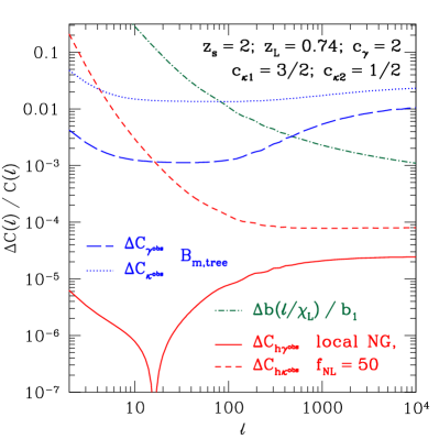
Figure 5: Relative correction to the halo-shear and halo-convergence cross power spectra from primordial NG of the local type (red solid/dashed). The blue long-dashed/dotted lines show the correction from the tree-level matter bispectrum from non-linear evolution in the absence of primordial non-Gaussianity. Here, we have assumed a lens redshift of $z_{L}=0.74$ and sources at $z_{s}=2$ so that $\chi_{s}=2\chi_{L}$. The dash-dotted line shows the correction to $C_{h\gamma},C_{h\kappa}$ from the scale-dependent halo bias Eq. (12) [via Eq. (36)], assuming $b_{1}=2$.

Fig. 5 shows the numerical result for Eqs. (37)–(38), assuming lens galaxies at $z_{L}=0.74$ and source galaxies at $z_{S}=2.0$. The redshift of the source galaxies is chosen by requiring $\chi_{s}=2\chi_{L}$. We assume that the linear bias parameter of lens galaxies is $b_{1}=2$, and the amplitude of non-Gaussianity is given by ${f_{\rm{NL}}}=50$. We adopt the same values for the non-linearity coefficients $c_{\gamma},c_{\kappa 1},c_{\kappa 2}$ as in the last section. We again see that the correction to $C_{h\gamma}$ is suppressed, while $C_{h\kappa}$ receives a correction that strongly increases towards large scales; in fact, at $\ell\lesssim 10$, the term $\propto\Delta b\>B_{I}\propto\ell^{-4}$ becomes larger than the contribution from the tree level matter bispectrum for these parameter values. Following similar steps to Sec. II, we can obtain an order of magnitude estimate of the nonlinear correction to $C_{h\kappa}$ from the local primordial bispectrum $B_{I}$ (for $C_{h\gamma}$ we again have a cosine factor which leads to a cancelation in the large-scale limit). Assuming the approximation of Eq. (24) we can write $\Delta C_{h\kappa^{\rm obs}}$ as

$$\Delta C_{h\kappa^{\rm obs}}(\ell)\approx\> \frac{4\,c_{\kappa}\,b_{1}\,{f_{\rm{NL}}}}{\mathcal{M}\left(\ell/\chi_{L};\>z_{L}\right)}C_{P}^{2}\,\left[\frac{D(z_{L})}{D(0)}\right]^{2}\,P_{L}\left(\frac{\ell}{\chi_{L}};z_{L}\right)$$

$$\times W^{2}_{L}(\chi_{s},\chi_{L})\frac{(1+z_{L})^{2}}{\chi_{L}^{2}}L_{P},$$ (41)

where $c_{\kappa}$ is defined below Eq. (29). Hence the relative correction to the tracer-convergence cross-correlation becomes

$$\frac{\Delta C_{h\kappa}(\ell)}{C_{h\kappa}(\ell)}\approx\> 4\,c_{\kappa}\,{f_{\rm{NL}}}\,(1+z_{L})\,D(z_{L})$$

$$\times\frac{C_{P}^{2}\,\chi_{L}^{2}\,W_{L}(\chi_{s},\chi_{L})\,L_{p}}{\ell^{\,2}\,T(\ell/\chi_{L})\,D^{2}(0)}\,.$$ (42)

Note that the bias factor $b_{1}+\Delta b(l/\chi_{L})$ drops out. In these expressions, a new length scale appears due to the projection,

$$L_{p}\equiv\int\frac{d^{2}k}{(2\pi)^{2}}P_{m}(k,z=0)\,.$$ (43)

$L_{p}$ can be seen as the one-dimensional coherence length of the density field at $z=0$, in the sense that the variance of the density field projected along a thin slab of thickness $\Delta\chi$ at redshift $z$ is given by

$$\sigma_{\delta\>\rm proj}^{2}=\left[\frac{D(z)}{D(0)}\right]^{2}\frac{L_{p}}{\Delta\chi}.$$ (44)

In our fiducial cosmology, $L_{p}=54.6\>\mathrm{Mpc}/h$.

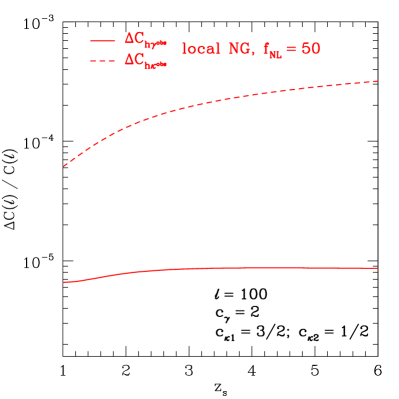
Figure 6: Relative amplitude of the non-linear lensing correction from primordial non-Gaussianity to the halo-shear and halo-convergence cross-correlation, as function of the lens redshift $z_{L}$, for a fixed multipole $\ell=100$. The other parameters are the same as for Fig. 5.

Since on large scales $T(\ell/\chi_{L})\approx 1$, Eq. (42) again recovers the $\ell^{-2}$ scaling of the non-linear correction, similar to what was found for the weak lensing power spectrum. Compared to the change in $C_{h\kappa}(\ell)$ due to the scale-dependent halo bias in Eq. (36) (green dot-dashed line in Fig. 5), which is exactly $1/2$ the effect on the halo angular power spectrum Eq. (31), the effect of the non-linear lensing correction is suppressed by a factor of

$$C_{P}W_{L}(\chi_{L},\chi_{s})L_{p}\sim L_{p}H_{0}\sim 0.02,$$ (45)

where we have assumed that $W_{L}$ is of order the horizon scale. While this is a significant reduction, the projection effect does not suppress the correction in galaxy-galaxy lensing quite as severely as it does for the shear power spectrum. This is mainly because in the cross-correlation with biased tracers the dominant contribution arises at $z_{L}$, rather than at low redshifts as in the lensing auto-correlation. Comparing with Fig. 5, the order of magnitude prediction again matches quite well.

Fig. 6 shows the amplitude of the corrections to $\Delta C_{h\kappa}$, $\Delta C_{h\gamma}$ as a function of source redshift. Here, we have chosen the lens redshift such that $\chi_{s}=2\chi_{L}$ in each case; thus maximizing the lensing kernel $W_{L}$. The scaling in redshift is very similar to that seen in the weak lensing power spectra, Fig. 3.

IV General statements on Peak clustering in Projected Fields

The results derived in the last two sections allow us to make some interesting and general statements on the effectiveness of using the clustering of peaks (or, more generally, non-linear tracers) identified in two-dimensional, projected density fields. Applications of this include shear peaks as well as peaks identified in diffuse background maps.

Consider a general projected density field

$$\lambda(\bm{\theta})\equiv\int d\chi F_{\lambda}(\chi)\delta(\chi\bm{\theta};\chi)\,,$$ (46)

where $F_{\lambda}(\chi)$ is a filter function normalized to unity in $\chi$. Using the Limber approximation, the angular power spectrum of $\lambda$ is then straightforwardly obtained as

$$C_{\lambda}(\ell)=\int\frac{d\chi}{\chi}\frac{F_{\lambda}^{2}(\chi)}{\chi}P_{m}\left(\frac{\ell}{\chi};\chi\right).$$ (47)

Now assume we identify peaks in $\lambda$; that is, we apply some nonlinear transformation so that the peak density is perturbatively given by

$$\lambda_{\rm pk}(\bm{\theta})=c_{1}\lambda(\bm{\theta})+\frac{c_{2}}{2}\lambda^{2}(\bm{\theta})+\cdots$$ (48)

The simplest example is thresholding, i.e. $\lambda_{\rm pk}(\bm{\theta})=\Theta(\lambda(\bm{\theta})-\lambda_{c})$, where $\Theta$ is the Heaviside function. If $\lambda_{c}\gg\sigma_{\lambda}$, $\sigma_{\lambda}$ being the r.m.s. fluctuation of $\lambda$ given by

$$\sigma_{\lambda}^{2}=\int\frac{d\chi}{\chi}\frac{F_{\lambda}^{2}(\chi)}{\chi}\int\frac{d^{2}\ell}{(2\pi)^{2}}P_{m}(\ell/\chi;\chi)\,,$$ (49)

$c_{1},\>c_{2}$ attain the well-known values Matarrese et al. (1986)

$$c_{1}=\frac{\lambda_{c}}{\sigma_{\lambda}^{2}};\quad c_{2}=c_{1}^{2}\,.$$ (50)

The following considerations are completely independent of the precise peak definition and value of $c_{2}$, however. Analogous to our derivations in Sec. II and III, the angular power spectrum of peaks can be written as

$$C_{\lambda_{\rm pk}}(\ell)=\> c_{1}^{2}\>C_{\lambda}(\ell)+\Delta C_{\lambda_{\rm pk}}(\ell)\,,$$

$$\Delta C_{\lambda_{\rm pk}}(\ell)=\> c_{1}c_{2}\int\frac{d^{2}\ell}{(2\pi)^{2}}B_{\lambda}(\ell,\ell_{1},|\ell_{1}-\ell|)\,.$$ (51)

The second term can in principle be used to probe primordial non-Gaussianity. We can now use the Limber approximation, and in the large scale limit make the same set of approximations as in the previous sections. As a further simplification, we will assume that the kernel $F_{\lambda}(\chi)$ is peaked at some distance $\bar{\chi}$. We then obtain the following estimate for the impact of non-Gaussianity on the clustering of peaks in the projected field $\lambda$:

$$\frac{\Delta C_{\lambda_{\rm pk}}(\ell)}{C_{\lambda_{\rm pk}}(\ell)}\approx\> 8f_{\rm NL}\frac{c_{2}\sigma_{\lambda}^{2}}{c_{1}}\frac{C_{P}\bar{\chi}^{2}}{\ell^{2}T(\ell/\bar{\chi})}\frac{1}{D(\bar{z})}$$

$$\approx\> 8f_{\rm NL}\frac{c_{2}}{c_{1}}\frac{C_{P}\bar{\chi}^{2}}{\ell^{2}T(\ell/\bar{\chi})\,D^{2}(0)}D(\bar{z})\frac{L_{p}}{\Delta\chi_{\lambda}}\,.$$ (52)

Here, $\bar{z}=z(\bar{\chi})$ and $\Delta\chi_{\lambda}\equiv[\int d\chi F_{\lambda}^{2}(\chi)]^{-1}$ is the effective width of the projection kernel. In the second line, we have introduced the correlation length $L_{P}$ via Eq. (44).

This result summarizes the different expressions for non-Gaussian corrections to angular power spectra derived in this paper: the first line of Eq. (52) clearly shows a strong similarity to the expression for halo clustering, Eq. (31), upon identifying $c_{2}\sigma_{\lambda}^{2}=c_{1}\delta_{c}$ from Eq. (50). Inserting the appropriate value for the width $\Delta\chi_{L}\equiv[C_{P}(1+z_{L})W_{L}]^{-1}$ of the lensing kernel (at fixed source redshift), setting $c_{1}=1,\;c_{2}=c_{\kappa}$, and dividing by a factor of 2 we also recover the expression for galaxy-galaxy lensing Eq. (42) (the factor of 2 comes in since Eq. (52) is for the auto-correlation while Eq. (42) is for a cross-correlation). Finally, we see that the quantity $\sigma_{\kappa}^{2}\sim L_{P}/\Delta\chi_{L}$ is suppressed by the same projection effect.

In summary, the clustering of peaks identified in the projected density field is suppressed relative to the angular clustering of peaks identified in the three-dimensional density field [Eq. (31)] by a factor of $D^{2}(\bar{z})\,L_{p}/\Delta\chi_{\lambda}$. In fact, if the kernel is broad, then the contributions to the bispectrum $B_{\lambda}$ are dominated by low redshifts, as we have seen in Sec. II, which further suppresses $\Delta C_{\lambda_{\rm pk}}$ beyond Eq. (52). Note that the Limber approximation and hence Eq. (52) break down if $\Delta\chi_{\lambda}\lesssim L_{p}$, i.e. for very narrow kernels.

Thus, unless the line-of-sight projection Eq. (46) can somehow be restricted to a range $\Delta\chi_{\lambda}\lesssim D^{2}(\bar{z})L_{p}\approx 54.6\,D^{2}(\bar{z})\,{\rm Mpc}/h$, the impact of primordial non-Gaussianity on the clustering of peaks identified in a projected density field is strongly suppressed.

V Conclusion

Observations of the large-scale structure in the Universe offer very promising opportunities for probing the initial conditions of the Universe, complementing the searches for deviations from Gaussianity in the temperature anisotropies of the cosmic microwave background. Weak lensing is one of the most powerful probes of large-scale structure, as it directly probes the underlying matter distribution, thus circumventing many of the uncertainties in the tracer-mass relation.

In this paper, we have shown that shear and convergence power spectra are in principle subject to corrections from primordial non-Gaussianity, since weak lensing estimators generally have non-linear corrections. However, projection effects severely reduce the impact of primordial non-Gaussianity, and the effects are generally much smaller than those from nonlinear gravitational evolution. This also holds when approximately including the effect of non-linear growth on small scales. We also investigate the same effects for galaxy-galaxy lensing, i.e. the cross-correlation of shear and convergence with some large-scale structure tracer. In this case, the suppression is somewhat mitigated, but still significant.

Finally, in Sec. IV we provide a general argument why this suppression is generic to searching for non-Gaussianity in two-dimensional projected density fields. If the projection occurs over a longer line-of-sight distance than the one-dimensional coherence length of the density field, $L_{P}\approx 54.6\>\,{\rm Mpc}/h$ (at $z=0$), the projected density field is more Gaussian than the underlying 3D density field, a consequence of the central limit theorem Scoccimarro et al. (1999). Thus, the effect of primordial non-Gaussianity on the clustering of peaks identified in such a projected density field is suppressed by $\sim L_{P}/\Delta\chi$, where $\Delta\chi$ is the width of the projection kernel. This applies to peaks identified in weak lensing shear maps (where $\Delta\chi\sim H_{0}$) as well as in diffuse backgrounds—unless a definite connection between such peaks and dark matter halos in the 3D density field can be made. Thus, we expect that the statistics of tracers of the 3D density field will generally provide tighter constraints on primordial non-Gaussianity than those of projected fields.