Kinematic Effect of Indistinguishability and Its Application
to Open Quantum Systems

Abstract

In quantum mechanics, useful experiments require multiple measurements performed on the identically prepared physical objects composing experimental ensembles. Experimental systems also suffer from environmental interference, and one should not assume that all objects in the experimental ensemble suffer interference identically from a single, uncontrolled environment. Here we present a framework for treating multiple quantum environments and fluctuations affecting only subsets of the experimental ensemble. We also discuss a kinematic effect of indistinguishability not applicable to closed systems. As an application, we treat inefficient photon scattering as an open system. We also create a toy model for the environmental interference suffered by systems undergoing Rabi oscillations, and we find that this kinematic effect may explain the puzzling Excitation Induced Dephasing generally measured in experiments.

I Introduction

It is because quantum theory makes probabilistic predictions that all quantitatively useful experiments require repeated measurements performed on identically prepared physical objects dirac_qm_book . These identically prepared physical objects constitute what we will call the experimental ensemble. And one cannot assume that all ensemble members, while treated identically by an experimenter, are also treated identically by an uncontrolled environment.

First we will explain what is meant by the experimental ensemble. Then to treat multiple quantum environments we will introduce a framework that one can use in addition to the typical reduced dynamics of open systems petruccione_open_quantum_systems . We will also explore a kinematic effect arising from the indistinguishability of different ensemble members. As applications, and to isolate the kinematics, we will work within the framework to model systems with either trivial or simple closed-system dynamics. We will treat as an open system the inefficient scattering of photons from a beam splitter. Then we will create a toy model for real experimental systems undergoing Rabi oscillations. We find that the general yet often puzzling phenomenon called Excitation Induced Dephasing results from the kinematics of indistinguishable ensemble members, and consequently we find very good quantitative agreement with a wide variety of experiments. For one well-known experiment meekhof_rabi_1996 , we find unprecedented quantitative agreement.

II Measurements and the Experimental Ensemble

The experimental ensemble is particularly easy to identify in modern experiments, such as nagourney_dehmelt_shelved_1986 ; bergquist_qjumps_1986 ; sauter_toschek_qjumps_1986 ; peik_qjumps_1994 ; meekhof_rabi_1996 ; brune_rabi_1996 , in which one repeatedly prepares, manipulates, and then measures the state of single physical objects, one at a time.

For example, in meekhof_rabi_1996 , a single beryllium ion is confined in a Paul trap. It is prepared to be in a motional and hyperfine ground state, and then a laser drives stimulated Raman transitions for a time duration, $t$, after which the state of the single ion is measured. Following that single observation, the preparation–evolution–measurement process is repeated. For every value of $t$ at which the experiment is performed, the result is the average of 4000 observations wineland_experimental_1998 . There is an experimental ensemble for every measured value of $t$, and in this example every ensemble has size 4000.

We offer these experiments only as clear illustrations of the experimental ensemble (though we will address meekhof_rabi_1996 and brune_rabi_1996 again in Section VI). Often multiple objects from the experimental ensemble are present simultaneously in the laboratory.

To generalize for systems and observables with discrete spectra, let $\lambda$ label a possible result of a quantum mechanical measurement. Assume that one performs $N$ measurements, and that the result $\lambda$ is found $n_{\lambda}$ times. The results of these measurements are counting ratios:

$$\frac{n_{\lambda}}{N}(t).$$ (1)

As is clear from experiments, the $t$ in (1) corresponds to a duration in time rather than to a time on the laboratory’s clock. Depending on the type of experiment, the ensemble size, $N$, may or may not be a function of $t$.

The $N$ measurements in (1) are performed on an experimental ensemble of $N$ identically prepared physical objects. Because individual measurements are always assumed to be independent of each other, the individual members of the experimental ensemble are assumed not to interact with each other. Thus the experimental ensemble must not be confused with a many-particle state having interacting components, for which useful measurements require an experimental ensemble of many-particle objects. A major subject of this study is whether or not the members can be considered also statistically independent in terms of exchange symmetry or other correlations. This will be discussed in detail later.

III Kinematic Aspects of Quantum Theory

One compares the experimental results in the form of (1) to theoretical probabilities. The theoretical image of any closed, quantum mechanical system is an operator algebra defined in a linear scalar-product space, $\Phi$. The vectors $\phi_{\alpha}$ span $\Phi$, and every linear combination of the $\phi_{\alpha}\in\Phi$ can possibly represent the state of the system. Assume that preparable states are represented by the basis vectors $\phi_{\alpha}$. In practice, one infers from a measurement or from a preparation procedure the state of an experimental system. From the $\phi_{\alpha}$ one constructs the appropriate density operator,

$$\rho(t)=\sum_{\alpha}w_{\alpha}|\phi_{\alpha}(t)\rangle\langle\phi_{\alpha}(t)|,\quad\textrm{with }\sum_{\alpha}w_{\alpha}=1,$$

to represent the inferred state of the closed system. In this paper, we will only consider systems for which $\alpha$ takes discrete values.

One characterizes an experimental observable by a prescription for how it is to be measured, and in the theory one represents it using a linear operator in $\Phi$. For simplicity and because it is appropriate for the experiments described above, we will consider a projection operator, $\Lambda=|\lambda\rangle\langle\lambda|$, into the one-dimensional subspace of $\Phi$ that is associated with the observable labeled above by $\lambda$. If $\lambda$ can be a value of the index $\alpha$, then the subspace spanned by $|\lambda\rangle\langle\lambda|$ will be spanned also by one of the $|\phi_{\alpha}\rangle\langle\phi_{\alpha}|$, such that the inner product $\langle\lambda|\phi_{\alpha}\rangle\propto\delta_{\alpha\lambda}$. It is straightforward to generalize to observables that do not have the $\phi_{\alpha}$ as eigenvectors.

These are kinematic aspects of quantum theory, and they are thus independent of any particular quantum system. The dynamics specific to a particular system enters the theory only through a concrete choice of the space $\Phi$ and of the operator algebra defined in it.

For projection operators such as $\Lambda$, the expectation value is the probability of finding the discrete value $\lambda$ in a measurement. The predictions of quantum theory are calculated in the form of Born probabilities, $\mathcal{P}_{\Lambda}\big{(}\rho(t)\big{)}$, where

$$\mathcal{P}_{\Lambda}\big{(}\rho(t)\big{)}=\mathrm{Tr}\big{(}\Lambda\,\rho(t)\big{)}.$$

The explicit comparison between experiment and theory is

$$\textrm{counting ratio}\equiv\frac{n_{\lambda}}{N}(t) \stackrel{{\scriptstyle?}}{{=}} \mathcal{P}_{\Lambda}\big{(}\rho(t)\big{)}\equiv\textrm{ Born probability}.$$ (2)

Experiment Theory

When comparing experimental results to theoretical predictions (2), increasing $N$ leads to stronger statistical conclusions regarding an inferred outcome, but increasing $N$ does not change the outcome itself. In other words, the theoretical predictions on the right hand side of (2) are always independent of the number of members in an ensemble, $N$, because no theoretical prediction should depend on the number of times one performs an experiment to verify it. A theory’s independence from $N$ is a necessary condition for the identification of the experimental ensemble.

IV Multiple Quantum Environments for a Single Experiment

Experimental systems cannot be perfectly isolated, and actual measurements always reveal the experimental signatures of environmental interference. In quantum theory there exist well-understood mechanisms to treat the interference between a quantum system and its environment petruccione_open_quantum_systems . The result is often a reduced dynamics, which can be used to calculate for an open system an increase in entropy or a loss of coherence.

One has typically not considered the possibility that different ensemble members might suffer interference from different environmental systems or from fluctuations within a single environmental system. That this possibility is relevant is especially obvious for the experiments described above nagourney_dehmelt_shelved_1986 ; bergquist_qjumps_1986 ; sauter_toschek_qjumps_1986 ; peik_qjumps_1994 ; meekhof_rabi_1996 ; brune_rabi_1996 , in which no two ensemble members are ever present simultaneously in the laboratory. Of course, because quantum theory describes physical phenomena independently of how many ensemble members are present simultaneously, then it must be relevant for all experiments and any number of simultaneously present members.

By ignoring the possibility that different ensemble members suffer interference differently, one implicitly assumes either that the uncontrolled environment treats them all identically or that experimenters can prepare and control the state of the entire environment. In practice, this is either unlikely or impossible.

IV.1 Different environments from the beginning

The simplest possibility for treating multiple quantum environments is to associate, for the entirety of the experiment, different ensemble members with different environmental systems. We will use $m$ to label these different environmental systems, $E_{m}$. The density operator representing the state of $E_{m}$ will be labeled $\rho_{E_{m}}$. The state of the subset of ensemble members suffering interference from the environmental system $E_{m}$ will be represented by $\rho_{m}$. One must also label the time evolution operator, $U_{m}(t)$, defined so that as a function of the duration, $t$, after active preparation, the time evolution of the composite of system and environment is

$$U_{m}(t)\,\rho_{m}\otimes\rho_{E_{m}}\,U^{\dagger}_{m}(t).$$

For a measurement performed at $t$, the states of the ensemble members are represented by the density operators

$$\rho_{m}(t)=\mathrm{Tr}_{E_{m}}\big{(}U_{m}(t)\,\rho_{m}\otimes\rho_{E_{m}}\,U^{\dagger}_{m}(t)\big{)},$$ (3)

where $\mathrm{Tr}_{E_{m}}$ denotes a partial trace over the degrees of freedom of the environmental system, $E_{m}$. This is the typical reduced dynamics for open systems petruccione_open_quantum_systems , but we have added the index $m$ to label the dynamics corresponding to the different environmental systems.

The density operator, $\rho(t)$, to be used in comparison with experimental data (2) is then

$$\rho(t)=\sum_{m=0}^{M}\,a_{m}\,\rho_{m}(t).$$ (4)

Here $M$ is the number of different environments deemed necessary for a model. So that the left hand side of (4) is a valid density operator, the real numbers $a_{m}$ in (4) must satisfy the convexity requirements

$$a_{m}\geq 0\quad\textrm{and}\quad\sum_{m=0}^{M}\,a_{m}=1.$$

IV.2 Interference events

With (4), any given ensemble member remains for the entirety of the experiment in the subset corresponding to a given environmental system. This will be problematic if there occur fluctuations in the environmental systems themselves, and the fluctuations affect only portions of subsets. We have assumed that members of the entire ensemble suffer interference differently, so we must assume also that members of any subset from (4) suffer differently. In a general treatment, there will be no fixed subsets of ensemble members.

To treat the possibility that members of any subset suffer environmental interference differently, one can assume that different fluctuations occur during different events throughout an experiment’s duration. Such events could describe something as simple as a temporary loss of homogeneity of a magnetic field. Another possibility for an interference event is the actual passive measurement of an observable in the state of an ensemble member. In the context of decoherence, Leggett has called this measurement process “garbling” leggett_arrow_qmeasurement .

We imagine the following sequence of interference events. Recall that, when treating actual data (2), and thus when representing the state of ensemble members, the $t$ represents a duration from active preparation. All members are therefore initially prepared at $t=0$.

1. A physicist actively prepares the initial state of all experimental ensemble members such that they are represented by a density operator labeled $\rho_{0}(t)$. At $t=t^{*}_{1}$ there occurs an interference event that cannot be described by the closed-system dynamics. If we ignore for now any finite duration of the event and any other source of environmental interference, then before the interference event ($0\leq t<t^{*}_{1}$) all ensemble members are represented by $\rho_{0}(t)$.

2. At $t=t^{*}_{1}$ the interference event affects some subset of the experimental ensemble. Because the closed-system dynamics cannot describe the interference, the affected members can no longer be represented by $\rho_{0}(t)$. Thus, to represent the state of the affected subset, one requires a new density operator: $\rho_{1}(t-t^{*}_{1})$. The unaffected members will continue to be in a state represented by $\rho_{0}(t)$.

3. If there is another interference event occurring at a duration $t_{2}^{*}$, then another density operator, $\rho_{2}(t-t^{*}_{2})$, will be required.

The density operator, $\rho(t)$, to be used in comparison with experimental data (2) will thus exhibit a branching behavior as time progresses:

$$\rho(\tilde{t})=\begin{cases}\rho_{0}(t_{0})&0\leq\tilde{t}<t^{*}_{1}\\ a_{0}\,\rho_{0}(t_{0})+a_{1}\,\rho_{1}(t_{1})&t^{*}_{1}\leq\tilde{t}<t_{2}^{*}\\ a_{0}\,\rho_{0}(t_{0})+a_{1}\,\rho_{1}(t_{1})+a_{2}\,\rho_{2}(t_{2})&t^{*}_{2}\leq\tilde{t}.\end{cases}$$ (5)

There is a notational complication here because the time parameter for experimental results, and thus the $t$ in (2), represents a duration from preparation. We will write $\tilde{t}$ on the left hand side to represent duration from active preparation of ensemble members. The branches on the right hand side of (5) will be functions of the different $t_{i}=t-t^{*}_{i}$, representing duration from the times $t^{*}_{i}$ when the $\rho_{i}$ became necessary. If the distinction is unnecessary, we will use $t$. For closed systems, this notation is not needed because $t_{i}\rightarrow t=\tilde{t}$.

Every line in (5) could be written in the same form as (4), but here $M$ would be the number of interference events. If there is a sequence of such events, say at $t^{*}_{i}$, then the number of density operators on the right hand side will depend on the time duration, $\tilde{t}$, and more and more branches will appear as the time duration grows.

Note that nothing new has been introduced to standard quantum mechanics, and that we have not assumed any new microphysical phenomena. In the absence of environmental interference, these approaches obviously reduce to the theory for closed systems. In the limit that all members suffer external interference identically, one has the typical formalism for open systems. All we have done differently is apply the standard theory to open systems in such a way that one can address the possibility that different ensemble members may suffer environmental interference differently. One should not read (5) to mean that the density operator undergoes a particular, dynamical change. Rather, this expression means that subsets of ensemble members suffer differently and therefore require different density operators to represent their states.

IV.3 The branching process

To represent the possibility that between $\tilde{t}$ and $\tilde{t}+\Delta\tilde{t}$ and before active measurement, some subset of the experimental ensemble suffers interference and afterward must be described by a new density operator, $\rho_{1}$, let us write from (5)

$$\rho_{0}(\tilde{t})\quad\longrightarrow\quad a_{0}\,\rho_{0}(\tilde{t}+\Delta\tilde{t})+a_{1}\,\rho_{1}(\tilde{t}+\Delta\tilde{t}).$$ (6)

Note that (6) is not mathematically correct. Let $\rho_{i}$ be constructed from vectors in the space $\Phi_{i}$. In $\Phi_{i}$ is defined the operator algebra representing the system’s dynamics following one particular type of environmental interference, which may not be defined in the space of the closed system itself. The dynamics of environmental interference is uncontrolled and may be unknown. In general, $\Phi_{i}\neq\Phi_{j\neq i}$, and one cannot perform the sum in (6). Instead, (6) is a phenomenological statement that is required because one can neither perfectly isolate experimental systems nor ensure that all ensemble members suffer interference identically.

While (6) might not make mathematical sense, it will have a sensible physical interpretation if the calculated probabilities are real numbers between 0 and 1. The corresponding expression for the Born probability is

$$\mathrm{Tr}\big{(}\Lambda_{0}\rho_{0}(\tilde{t})\big{)} \longrightarrow a_{0}\,\mathrm{Tr}\big{(}\Lambda_{0}\rho_{0}(\tilde{t}+\Delta\tilde{t})\big{)}$$ (7)

$$+\,a_{1}\,\mathrm{Tr}\big{(}\Lambda_{1}\rho_{1}(\tilde{t}+\Delta\tilde{t})\big{)}.$$

To calculate Born probabilities one must decide how the operators $\Lambda_{i}$ or $\rho_{i}$ might be extended or limited to other spaces such that this requirement is fulfilled. For the remainder of this paper, we will assume that this can be done. Again, the weights, $a_{0}$ and $a_{1}$, in (6) and  (7) must satisfy $a_{0}+a_{1}=1$.

We have ignored any dynamics hidden by the arrow in (6). If the timescale associated with the interference event, $\Delta\tilde{t}$ in (6), is very small compared to the dynamical timescales of the experiment, then one can safely ignore it. If it is not, then in models one must include interference dynamics along with the regular system dynamics.

IV.4 Partitioning and indistinguishability

Finally, let us consider the weights, $a_{i}$, in (4) and (5). The $a_{i}$ express the relative sizes of the ensemble’s different subsets, which are in states represented by the different $\rho_{i}$. To determine the relative sizes of these subsets, one must partition an ensemble of arbitrary size, $N$.

To complicate matters, there is a kinematic requirement that limits one’s knowledge of which members suffer interference from which environments. When the spatial wave functions of $n$ simultaneously present ensemble members overlap, any $n$-body wave function must transform as one of the irreducible representations of the permutation group of order $(n!)$. Even if the non-interacting ensemble members are sufficiently spaced that particle statistics can be ignored, when an external system cannot distinguish them, interactions still must respect a permutation symmetry. It is this condition that leads to the well-known phenomenon of super-radiance dicke_superrad_1954 . This phenomenon has previously been investigated in the context of open systems lidar_decofree_2001 and called collective decoherence, in which a bath (environment) cannot distinguish between $n$ qubits. Here we have generalized to allow multiple baths, and we will attempt to treat the case that $n$ varies and is not known.

Clearly, if one does not know $n$, then one cannot explicitly address a permutation symmetry when determining the $a_{i}$. The physical interpretation of the permutation symmetry is that some simultaneously present members of the ensemble are indistinguishable and cannot be given physically meaningful labels.

We conclude with a set of restrictions on partitioning:

1. $\rho$ represents the state of an arbitrary number, $N$, of ensemble members (see Section III).

2. Subsets are therefore also of arbitrary size.

3. One cannot explicitly address the number of ensemble members simultaneously affected by a single, uncontrolled environment.

4. One cannot give individual ensemble members a physically meaningful label.

These restrictions seem to prevent one from avoiding partitioning by defining within a standard reduced dynamics any single, “effective” environment or any interaction operator that dynamically mimics the kinematic effects of indistinguishability for the average ensemble member. In the next two sections, we will use the framework to treat different physical systems. To isolate the effects of kinematics, in Section V we create a model with trivial dynamics, and in Section VI we create a model with simple dynamics.

V Application: Beam Splitter

Consider the simple system of a photon, $\gamma$, incident on a beam splitter, being either transmitted into one phototube or else reflected into a different phototube. Figure 1 is a schematic of the experiment.

Figure 1: Schematic of the photon scattering experiment. It is divided into System $A$, the incident photons, and System $B$, the reflected and transmitted photons. Reflected photons are registered by phototube 1, and transmitted photons are registered by phototube 2. Not shown is an imagined source incident from the top.

The photon scattering system is interesting as the basis of a photon current. The probabilistic nature of the scattering at the beam splitter is for the photon current a source of noise buttiker_92 characterized by correlations between photons in the transmitted and reflected branches.

V.1 Second quantization calculation

Second quantization provides a simple and effective framework for calculating correlations, in terms of occupation numbers in the incident, transmitted, and reflected currents. In the next section we will use our framework and compare to the results of this section. We are not interested in the microscopic scattering dynamics for a photon incident on a beam splitter, so following loudon_91 for this simple case we will deal only with asymptotic in and out states at fixed energy, and ignore other quantum numbers.

One comment is required, however. Because the scattering operator, $\hat{S}$, does not change the space of asymptotic states, one requires another input channel in Figure 1, corresponding to photons incident from the top. Such photons, were they present, would transmit into phototube 1 and reflect into phototube 2. This imagined photon source is not present in the actual experiment, however, so one fixes its input as the vacuum state. Though it emits no photons, only when the imagined photon source is present in the calculation does one calculate the correct values for the correlation functions loudon_91 .

To preserve the symmetry implied by the theoretical approach, let us temporarily change the input system to include this imagined source. The creation and annihilation operators for incoming photons will be $\hat{a}^{\dagger}_{i}$ and $\hat{a}_{i}$, where $i=1,2$, and

$$[\hat{a}_{i},\hat{a}_{j}^{\dagger}]=\delta_{ij}.$$ (8)

The actual source, seen in Figure 1, will correspond to $i=1$, and the imagined source will correspond to $i=2$.

For photons in the reflected and transmitted currents, one defines the creation and annihilation operators, $\hat{b}^{\dagger}_{i}$ and $\hat{b}_{i}$, with $i=1,2$ corresponding to the label on the phototubes in Figure 1, and also satisfying (8).

The reflection or transmission at the beam splitter is then treated as a scattering event, and one can relate the incoming photons to the transmitted and reflected photons by buttiker_92 ,

$$\left(\begin{array}[]{c}\hat{b}_{1}\\ \hat{b}_{2}\\ \end{array}\right)=\left(\begin{array}[]{cc}r_{1\,1}&t_{1\,2}\\ t_{2\,1}&r_{2\,2}\\ \end{array}\right)\left(\begin{array}[]{c}\hat{a}_{1}\\ \hat{a}_{2}\\ \end{array}\right).$$ (9)

Here the unitary scattering matrix is written in terms of the complex reflection coefficient, $r$, and the complex transmission coefficient, $t$, which satisfy $|r|^{2}+|t|^{2}=1$. The vacuum state for the input photons is $|0\rangle_{1}|0\rangle_{2}\equiv|0\rangle$. We will consider an input state, $|n\rangle$, containing $n$ photons emitted by the actual source, $i=1$, so that

$$|n\rangle=\frac{(\hat{a}_{1}^{\dagger})^{n}}{\sqrt{n!}}|0\rangle.$$ (10)

Following buttiker_92 , we let $|r_{11}|^{2}\equiv R$ and $|t_{21}|^{2}\equiv T$, and we assume unit efficiencies for measurement. The operator representing the occupation number in the reflected channel of Figure 1 is $\hat{n}_{R}=\hat{b}^{\dagger}_{1}\hat{b}_{1}$, and the the operator representing the occupation number in the transmitted channel of Figure 1 is $\hat{n}_{T}=\hat{b}^{\dagger}_{2}\hat{b}_{2}$. Using (9) and (10), one calculates for the correlations between occupation numbers:

$$\langle\hat{n}_{R}\hat{n}_{T}\rangle = \langle n|\hat{b}^{\dagger}_{1}\hat{b}_{1}\hat{b}^{\dagger}_{2}\hat{b}_{2}|n\rangle=RTn(n-1)$$

$$\langle\hat{n}_{R}\rangle = nR$$

$$\langle\hat{n}_{T}\rangle = nT$$ (11)

$$\langle(\Delta\hat{n}_{R})^{2}\rangle = \langle(\Delta\hat{n}_{T})^{2}\rangle=nRT$$

$$\langle\Delta\hat{n}_{R}\Delta\hat{n}_{T}\rangle = -nRT$$

V.2 Scattering as an interference event

In this section we will begin to work within the open systems framework of Section IV, and in the next section we will introduce losses. The scattering system of Figure 1 is naturally divided at the beam splitter, into subsystems:

1. System $A$, which includes the incident photons:
   The density operator $\rho_{A}(t)$ represents the state of the incident photons. It is defined in the linear scalar-product space $\Phi_{A}$, which is spanned by the ket $|i\rangle$. In this basis, $\rho_{A}=|i\rangle\langle i|$. The Hamiltonian operator is $H_{A}$, and System $B$ is external, so we assume trivial dynamics with $[\rho_{A},H_{A}]=0$.

2. System $B$, which includes the reflected and transmitted photons:
   The density operator for a single photon, $\rho_{B}(t)$, is defined in the space $\Phi_{B}$, which is spanned by the orthogonal kets $|r\rangle$, representing the state of reflected photons, and $|t\rangle$, representing the state of transmitted photons. The Hamiltonian operator is $H_{B}$, and the dynamics is again trivial, with $[\rho_{B},H_{B}]=0$.

To measure the expectation values in (V.1), one actively prepares $n$ photons simultaneously in the incident channel. The $n$ photons then scatter from the beam splitter, and one measures the state of the $n$ photons by counting the numbers registered in phototubes 1 and 2. If one performs $N$ measurements, then one has identically prepared the state of $n$ photons a total of $N$ times.

Every incident photon is actively prepared in a state represented by $\rho_{A}=|i\rangle\langle i|$. Eventually every photon reaches the beam splitter and is scattered, which is the interference event during which the uncontrolled environment passively prepares every photon such that its state must be described by $\rho_{B}$. According to the framework proposed in Section IV, in addition to the typical reduced dynamics, density operators undergo the branching

$$\rho_{A}(t)\longrightarrow w_{A}\,\rho_{A}(t+\Delta t)+w_{B}\,\rho_{B}(t+\Delta t)$$ (12)

whenever subsets of ensemble members are passively prepared by an uncontrolled environment. All dynamics for in and out states is trivial, so we will drop the time dependence from equations in this section.

The scattering matrix in (9) preserves photon number loudon_91 . From this we deduce for (12) that $w_{A}+w_{B}=1$. For the simple scattering experiment in which one assumes unit efficiencies, all photons are eventually scattered into states in System $B$. We can therefore deduce further that $w_{A}=0$, fixing $w_{B}=1$.

If one knows the scattering theory (9) for the passive preparation of photons by the beam splitter, then one can write for $n=1$

$$\rho_{A}\longrightarrow\rho_{B} = R\,|r\rangle\langle r|+T\,|t\rangle\langle t|$$ (13)

$$+r_{1\,1}t^{*}_{2\,1}\,|r\rangle\langle t|+t_{2\,1}r^{*}_{1\,1}\,|t\rangle\langle r|.$$

By assuming the most general form for $\rho_{B}$, one would also arrive at (13) up to the coefficients. For this example with trivial dynamics, the framework simply reproduces an expression (13) commonly used in the study of quantum optics gerry_optics_book . The only difference for our framework is that (13) represents the state of only the $n=1$ subset of the experimental ensemble.

Of course, one often will not know the complete theory for passive preparations by an unknown environment. The measurements that lead to (V.1) are not sensitive to entanglement, and the dependence of the correlation functions on $n$ is entirely kinematic.

Without more sophisticated measurements or a complete scattering theory, by imagining that a physicist actively prepares any number of photons in a sequence $n_{j}$, $j=1,2,3\ldots$, one can deduce a form for $\rho_{B}$ that, though incomplete, is consistent with (V.1). For any sequence $n_{j}$, the probability that any given photon is reflected is

$$\sum_{j}\left(\frac{\langle\hat{n_{j}}_{R}\rangle}{n_{j}}\right)=R=\mathcal{P}_{R}(\rho_{B}).$$

After an incident photon is scattered, then, the probability to find it in the reflected channel is

$$\mathcal{P}_{R}(\rho_{B})=\mathrm{Tr}\left(|r\rangle\langle r|\,\rho_{B}\right)=R.$$ (14)

Similarly, the probability to find the photon in the transmitted channel is

$$\mathcal{P}_{T}(\rho_{B})=\mathrm{Tr}\left(|t\rangle\langle t|\,\rho_{B}\right)=T.$$ (15)

Knowing (14) and (15) from measurements, and without knowing about the entanglement in (13), one deduces for (12)

$$\rho_{A}\longrightarrow\rho_{B}=R\,|r\rangle\langle r|+T\,|t\rangle\langle t|.$$ (16)

We are interested in exploring the kinematics of indistinguishability without knowing the number, $n$, of photons present, and therefore not concerned with entanglement. If the beam splitter is to represent an unknown environment, when developing models one presumably would not even know about entanglement or the imagined photon source. For the remainder of this section we will ignore off-diagonal elements of the density operator (13) and restrict ourselves to operators of the form (16).

In (16) we have also ignored the kinematics associated with the simultaneous presence of $n$ incident photons. One cannot start with (16) and directly calculate the correlation functions in (V.1). One way to include the kinematic information is to write the analogue of (16) for $n$ incident photons. This is demonstrated in Appendix A for $n=3$. Here we will show for general $n$ that by counting indistinguishable reflection events and indistinguishable transmission events, one can instead partition the experimental ensemble represented by $\rho_{B}$ in (16) into an ensemble of $n$-photon objects while respecting permutation symmetry and the requirements of Section IV.4.

Each of the single photons is passively prepared with probability $R$ to be in the state $|r\rangle$ and with probability $T$ to be in the state $|t\rangle$. The ensemble members are otherwise indistinguishable, so to partition the ensemble we will use the binomial distribution,

$$\binom{n}{k}R^{k}T^{n-k},$$

to average over the partitions containing combinations of $k$ indistinguishable photons reflected with probability $R$ and $(n-k)$ indistinguishable photons transmitted with probability $T$.

The expectation values $\langle\hat{n}_{R}\rangle$ and $\langle\hat{n}_{T}\rangle$ are then related to the first moment of the binomial distribution. We calculate

$$\langle\hat{n}_{R}\rangle=\sum_{k=0}^{n}\binom{n}{k}R^{k}T^{n-k}k=nR,$$ (17)

and

$$\langle\hat{n}_{T}\rangle=\sum_{k=0}^{n}\binom{n}{k}R^{k}T^{n-k}(n-k)=nT.$$ (18)

In this method, we put $k$ inside the summation to represent the number of photons reflected. We put $(n-k)$ inside the summation to represent the number of photons transmitted. Therefore $\langle\hat{n}_{R}\hat{n}_{T}\rangle$ is

$$\langle\hat{n}_{R}\hat{n}_{T}\rangle = \sum_{k=0}^{n}\binom{n}{k}R^{k}T^{n-k}k(n-k)=RTn(n-1).$$ (19)

For the remaining relations, we find

$$\langle(\Delta\hat{n}_{R})^{2}\rangle = \sum_{k=0}^{n}\binom{n}{k}R^{k}T^{n-k}(k-nR)^{2}=nRT$$ (20)

$$\langle(\Delta\hat{n}_{T})^{2}\rangle = \sum_{k=0}^{n}\binom{n}{k}R^{k}T^{n-k}\big{(}(n-k)-nT\big{)}^{2}=nRT$$ (21)

$$\langle\Delta\hat{n}_{R}\Delta\hat{n}_{T}\rangle = \sum_{k=0}^{n}\binom{n}{k}R^{k}T^{n-k}(k-nR)\big{(}(n-k)-nT\big{)}=-nRT,$$ (22)

as expected from (V.1). Though we have not yet introduced losses or dynamics, we have treated the scattering event as an interference event, and we have partitioned an experimental ensemble.

V.3 Open systems and inefficiencies

With the generalization of the theory of open systems and the partitioning method of Section V.2, it is straightforward to introduce losses into the photon scattering system. We will consider two sources of inefficiency. The first occurs if photons are scattered toward the phototubes of Figure 1 but the phototubes fail to register the photons. Unless one models the detector quantum mechanically, detector inefficiency does not require an open system treatment. Let $\Lambda_{R}^{\prime}$ be the operator representing observation of reflected photons, and let $\Lambda_{T}^{\prime}$ represent observation of transmitted photons. If there is some probability of a failed registration, then one has

$$\Lambda_{R}^{\prime}\Rightarrow(1-\epsilon_{R})|r\rangle\langle r|\quad\textrm{and}\quad\Lambda_{T}^{\prime}\Rightarrow(1-\epsilon_{T})|t\rangle\langle t|,$$

where $\epsilon_{R}$ is the probability that a photon fails to register in phototube 1, and $\epsilon_{T}$ is the probability that a photon fails to register in phototube 2. The probability to measure a reflected photon is

$$\mathcal{P}_{R}\big{(}\rho_{B}\big{)}=(1-\epsilon_{R})R,$$

and the probability to measure a transmitted photon is

$$\mathcal{P}_{T}\big{(}\rho_{B}\big{)}=(1-\epsilon_{T})T.$$

The second type of inefficiency occurs when the beam splitter scatters photons into such directions that they will not hit either phototube. Then one introduces another system, System $C$, that includes these photons. System $B$ is the system of interest, and System $C$ corresponds to the environmental system of the typical framework petruccione_open_quantum_systems . Unmeasurable photons are in a state represented by a density operator, $\rho_{C}$, constructed from vectors in the space $\Phi_{C}$, which does not contain $|r\rangle$ or $|t\rangle$. Instead of (16), one uses

$$\rho_{A} \longrightarrow w_{B}\,\rho_{B}+w_{C}\,\rho_{C}$$ (23)

$$=w_{B}\big{(}R|r\rangle\langle r|+T|t\rangle\langle t|\big{)}+w_{C}\,\rho_{C}$$

to represent passive preparation at the beam splitter (again ignoring entanglement).

It is important to note again that (23) is not mathematically correct because $\rho_{B}$ and $\rho_{C}$ are not defined in the same space. The probability after scattering to measure the observable represented by $\Lambda$ is

$$\mathcal{P}_{\Lambda_{B}}\big{(}w_{B}\rho_{B}\big{)}+\mathcal{P}_{\Lambda_{C}}\big{(}w_{C}\rho_{C}\big{)}\qquad$$

$$=w_{B}\mathcal{P}_{\Lambda_{B}}\big{(}\rho_{B}\big{)}+w_{C}\mathcal{P}_{\Lambda_{C}}\big{(}\rho_{C}\big{)},$$ (24)

where $w_{B}+w_{C}=1$, and $\Lambda_{C}$ is the appropriate operator in the space $\Phi_{C}$. Because System $C$ contains photons that are not measured, $\Lambda_{C}$ is the zero operator in $\Phi_{C}$. The probability to measure a reflected photon is

$$\mathcal{P}_{R}\big{(}w_{B}\rho_{B}\big{)}=w_{B}R,$$

and the probability to measure a transmitted photon is

$$\mathcal{P}_{T}\big{(}w_{B}\rho_{B}\big{)}=w_{B}T.$$

In real experiments, both sources of measurement inefficiency will appear, and one will have for the probabilities

$$\mathcal{P}_{R}\big{(}\rho_{B}\big{)}=w_{B}(1-\epsilon_{R})R$$

and

$$\mathcal{P}_{T}\big{(}\rho_{B}\big{)}=w_{B}(1-\epsilon_{T})T.$$

Now we can check the results in (V.1), for the case that one does not have unit efficiencies. Let $R^{\prime}$ be the probability that a reflected photon is registered and $T^{\prime}$ be the probability that a transmitted photon is registered. Let $\eta$ be the probability that an ensemble member is not measured, such that

$$R^{\prime}+T^{\prime}+\eta=1.$$ (25)

If the experimental ensemble contains all photons actively prepared in the incident channel, then

$$R^{\prime} = w_{B}(1-\epsilon_{R})R$$

$$T^{\prime} = w_{B}(1-\epsilon_{T})T$$ (26)

$$\eta = 1-w_{B}(1-\epsilon_{R}R-\epsilon_{T}T).$$

If, instead, the experimental ensemble contains only those photons scattered into System $B$, then $w_{B}=1$, and

$$R^{\prime} = (1-\epsilon_{R})R$$

$$T^{\prime} = (1-\epsilon_{T})T$$ (27)

$$\eta = \epsilon_{R}R+\epsilon_{T}T.$$

In general, one will not know if a photon remains unmeasured because of inefficiencies in scattering or because of inefficiencies in the phototubes. In other words, one can measure $R^{\prime}$ and $T^{\prime}$, but one will not know which of (V.3) or (V.3) is appropriate.

In (23) we have the theory for the state of any single photon before and after an interference event. To calculate correlation functions for different $n$, again we partition the experimental ensemble. Now we must use the multinomial distribution:

$$\langle\hat{n}_{R}\rangle = \sum_{j=0}^{n}\sum_{k=0}^{n}\sum_{\ell=0}^{n}\frac{n!}{j!k!\ell!}R^{\prime j}T^{\prime k}\eta^{\prime\ell}\,\delta_{n,j+k+\ell}\,j=nR^{\prime}(R^{\prime}+T^{\prime}+\eta)^{n-1}$$ (28)

$$\langle\hat{n}_{T}\rangle = \sum_{j=0}^{n}\sum_{k=0}^{n}\sum_{\ell=0}^{n}\frac{n!}{j!k!\ell!}R^{\prime j}T^{\prime k}\eta^{\prime\ell}\,\delta_{n,j+k+\ell}\,k=nT^{\prime}(R^{\prime}+T^{\prime}+\eta)^{n-1}$$ (29)

$$\langle\hat{n}_{R}\hat{n}_{T}\rangle = \sum_{j=0}^{n}\sum_{k=0}^{n}\sum_{\ell=0}^{n}\frac{n!}{j!k!\ell!}R^{\prime j}T^{\prime k}\eta^{\prime\ell}\,\delta_{n,j+k+\ell}\,jk=R^{\prime}T^{\prime}n(n-1)(R^{\prime}+T^{\prime}+\eta)^{n-2}$$ (30)

where $\delta_{n,j+k+\ell}$ is the Kronecker delta. Because of (25), we have $\langle\hat{n}_{R}\rangle=nR^{\prime}$, $\langle\hat{n}_{T}\rangle=nT^{\prime}$, and $\langle\hat{n}_{R}\hat{n}_{T}\rangle=R^{\prime}T^{\prime}n(n-1)$.

Using (25), the other expectation values are

$$\langle(\Delta\hat{n}_{R})^{2}\rangle = \sum_{j=0}^{n}\sum_{k=0}^{n}\sum_{\ell=0}^{n}\frac{n!}{j!k!\ell!}R^{\prime j}T^{\prime k}\eta^{\prime\ell}\,\delta_{n,j+k+\ell}\,(j-nR^{\prime})^{2}=nR^{\prime}(T^{\prime}+\eta)$$ (31)

$$\langle(\Delta\hat{n}_{T})^{2}\rangle = \sum_{j=0}^{n}\sum_{k=0}^{n}\sum_{\ell=0}^{n}\frac{n!}{j!k!\ell!}R^{\prime j}T^{\prime k}\eta^{\prime\ell}\,\delta_{n,j+k+\ell}\,(k-nT^{\prime})^{2}=nT^{\prime}(R^{\prime}+\eta)$$ (32)

$$\langle\Delta\hat{n}_{R}\Delta\hat{n}_{T}\rangle = \sum_{j=0}^{n}\sum_{k=0}^{n}\sum_{\ell=0}^{n}\frac{n!}{j!k!\ell!}R^{\prime j}T^{\prime k}\eta^{\prime\ell}\,\delta_{n,j+k+\ell}\,(j-nR^{\prime})(k-nT^{\prime})=-nR^{\prime}T^{\prime}$$ (33)

Comparing (28)–(33), where $R^{\prime}+T^{\prime}+\eta=1$, one can see how to generalize to imperfect measurements the results (V.1) of Section V.1, where $R+T=1$ and inefficiencies were ignored. The main difference is that $\langle(\Delta\hat{n}_{R})^{2}\rangle\neq\langle(\Delta\hat{n}_{T})^{2}\rangle$ when $\eta\neq 0$. If one writes from (V.1) that $\langle(\Delta\hat{n}_{R})^{2}\rangle=nR(1-R)$ and $\langle(\Delta\hat{n}_{T})^{2}\rangle=nT(1-T)$, however, then one can correctly take $R\rightarrow R^{\prime}$ and $T\rightarrow T^{\prime}$.

In the language of the theory of open systems petruccione_open_quantum_systems , the system of interest includes measurable photons in states described by $\rho_{B}$, which is constructed from vectors in $\Phi_{B}$. The environment contains unmeasurable photons in states described by $\rho_{C}$, which is constructed from vectors in $\Phi_{C}$. All scattered photons are represented by vectors in $\Phi=\Phi_{B}\oplus\Phi_{C}$, which is the space of states of the combined “system plus environment,” when entanglement with the environment is ignored.

In scattering experiments, one does not measure a dynamical dissipation in currents. In (16) and (23) we therefore have models without dynamics. Inefficiencies appear as a measurement event rate smaller than the incidence rate per area of incoming objects, for a given cross section. While an experimenter continues to supply photons, the losses appear only as measurement inefficiencies, which are treated by normalizing measured data to the total number of photons registered in the phototubes over the course of the experiment.

VI Application: Rabi Oscillations Experiments

As an application with simple dynamics, we will create a toy model for systems undergoing Rabi oscillations. Here time cannot be ignored, and we must deduce a form for environmental interactions. We will also implement the technique used in the previous section to partition the ensemble of single photons represented by (16) into an ensemble of $n$-photon objects.

VI.1 Rabi Oscillations

The theory of Rabi oscillations is well established dodd_atoms_1991 . It describes a two level system, with levels described by the projection operators $|g\rangle\langle g|$ representing the ground state and $|e\rangle\langle e|$ representing the excited state. When the system is prepared at $t=0$ to be in the excited state, $|e\rangle$, and it is coupled to a correctly tuned radiation field, the probability at $t$ to find the system in the ground state, $|g\rangle$, is

$$\mathcal{P}_{|g\rangle\langle g|}\big{(}\rho(t)\big{)}=\textrm{sin}^{2}(\Omega t)=\frac{1}{2}\big{(}1-\textrm{cos}(2\Omega t)\big{)},$$ (34)

where $\Omega$ is called the Rabi frequency. (The probability to find the system in the same state in which it was prepared is $\textrm{cos}^{2}(\Omega t)$.) These expressions are calculated using the dynamics for closed systems undergoing Rabi oscillations. The probability in (34) is to be compared with experimental results (2).

In actual experiments, because of environmental interference one never measures the result in (34). In this paper we wish to consider several very different but very clean and well-controlled experiments meekhof_rabi_1996 ; brune_rabi_1996 ; petta_coherent_2005 ; cole_nature_2001 ; zrenner_nature_2002 ; wang_macdonald_prb_2005 ; ramsay_prl_2010 .

In one experiment meekhof_rabi_1996 , also discussed in Section II, internal levels of a ⁹Be⁺ ion couple to the harmonic binding potential. Rabi oscillations occur between two of the coupled internal and vibrational levels, and the oscillations between different sets of levels are measured. In another experiment brune_rabi_1996 , Rabi oscillations are observed between the circular states of a Rydberg atom coupled to a field stored in a high $Q$ cavity. In petta_coherent_2005 , the Rabi oscillations are between the spin states of two electrons in a double quantum dot. In cole_nature_2001 , Rabi oscillations occur between motional states of electrons bound to shallow donors in semiconductors. These motional states mimic the levels of a hydrogen atom. In three experiments zrenner_nature_2002 ; wang_macdonald_prb_2005 ; ramsay_prl_2010 , oscillations occur between excitation levels of electrons confined in quantum dots.

The measured results in meekhof_rabi_1996 ; brune_rabi_1996 ; petta_coherent_2005 , do not match the prediction in (34). Instead, the measured probability is fit by an appropriately damped sinusoid that is a function of the time duration, $\tilde{t}$, from active preparation,

$$\mathcal{P}_{|g\rangle\langle g|}\big{(}\rho(\tilde{t})\big{)}=\frac{1}{2}\big{(}1-e^{-\gamma\tilde{t}}\,\textrm{cos}(2\Omega\tilde{t})\big{)},$$ (35)

where $\gamma$ is an experimentally determined damping factor.

In petta_coherent_2005 , amplitude, offset, and phase are fit as well, because the oscillations are measured also as a function of a swept detuning voltage. In wang_macdonald_prb_2005 ; ramsay_prl_2010 , photocurrent is measured, and from it the dephasing of the Rabi oscillations is inferred. Numerically solving the models they fit to their data, the subsystems undergoing Rabi oscillations fit (35).

VI.2 Dynamics for the toy model

Already having the kinematic requirements for open systems and indistinguishable ensemble members, our next task is to deduce the proper dynamics for the experimental system in question. This means we must identify the spaces $\Phi_{i}$ and the corresponding algebras of observables. Starting with the branched density operator from (5), we calculate the probability at a duration $\tilde{t}$ from active preparation:

$$\mathcal{P}_{\Lambda}\big{(}\rho(\tilde{t})\big{)} = \mathrm{Tr}\big{(}\Lambda_{0}\,a_{0}\,\rho_{0}(t_{0})\big{)}+\mathrm{Tr}\big{(}\Lambda_{1}\,a_{1}\,\rho_{1}(t_{1})\big{)}+\ldots$$ (36)

$$= a_{0}\,\mathcal{P}_{\Lambda_{0}}\big{(}\rho_{0}(t_{0})\big{)}+a_{1}\,\mathcal{P}_{\Lambda_{1}}\big{(}\rho_{1}(t_{1})\big{)}+\ldots\,\,\,\,\,\,$$

where, as before, $\rho_{i}$ is constructed from vectors in $\Phi_{i}$.

For the long-time behavior of the measured result in (35), one has

$$\lim_{\tilde{t}\rightarrow\infty}\mathcal{P}_{|g\rangle\langle g|}\big{(}\rho(\tilde{t})\big{)}=\frac{1}{2}.$$

From this we deduce that there is no dissipation for the experimental system, and that the terms $\mathcal{P}_{\Lambda_{i}}\big{(}\rho_{i}(t_{i})\big{)}$ in (36) ought not to introduce the type of losses considered for the beam splitter in Section V.3. For these experiments, we then hypothesize that immediately after the interference event, $\Phi_{0}=\Phi_{1}=\Phi_{i}$ for all $i$, so we can take $\Phi_{i}\rightarrow\Phi$. The algebra of observables will therefore be the typical algebra for the closed system, so we will take $\Lambda_{i}\rightarrow\Lambda=|g\rangle\langle g|$. We want a probability of the form

$$\mathcal{P}_{\Lambda}\big{(}\rho(\tilde{t})\big{)}=\sum_{m=0}^{M_{branch}}\,a_{m}\,\mathcal{P}_{\Lambda}\big{(}\rho_{m}(t_{m})\big{)}$$ (37)

where $M_{branch}$ is the number of branches. To keep track of the branches, we will find it convenient to retain the label $i$ for the $\rho_{i}$, even though all $\rho_{i}$ are defined in the same space, $\Phi$. This formula is deceptively simple in appearance, because, in general, the number of branches, $M_{branch}$, will depend on $\tilde{t}$, and the value of $a_{m^{\prime}}$ for a fixed $m^{\prime}$ will depend on $M_{branch}$.

The $\rho_{i}$ are all defined in $\Phi$, and to keep our model simple we will assume that during interference events the environment prepares the system to be in energy eigenstates, $|g\rangle$ and $|e\rangle$, ignoring entanglement. When a passive preparation occurs at $t_{i}=0$, the most general form for $\rho_{i}$ in (5) is then

$$\rho_{i}(t_{i}=0)=w_{i}\,\,|g\rangle\langle g|+v_{i}\,\,|e\rangle\langle e|,$$ (38)

with $w_{i}+v_{i}=1$. In (38), $w$ is a weight appropriate for ensemble members prepared passively to be in the ground state, and $v$ is a weight for ensemble members prepared in the excited state.

Note that this is not a new idea. Leggett has suggested leggett_arrow_qmeasurement that decoherence “is exactly the result of a ‘measurement’ whose result is uninspected,” and he has called this process “garbling.” With this toy model, developed within our framework, we will treat the effects of garbling. We ignore the dynamics of the measurement process itself because it is simply not understood and apparently occurs over very small durations in time.

VI.3 Born probability

For simplicity, we will assume that the passive measurements for our systems are fair measurements, though this would not generally be required. To isolate kinematic effects, we will also ignore any reduced dynamics expressed in (3) and (4).

When modeling experiments or using more sophisticated models for environmental interaction, one would probably use a full simulation. To maintain transparency, however, we will search for an analytical formula for our toy model. We will start with a sequence of interference events described in Section IV.2. Because the damping of the oscillations in (35) is exponential, the decay rate is constant, and we can deduce that there should be a single timescale, $\Delta\tilde{t}$, for regularly spaced interference events. Then the Born probability when there may have been $n$ interference events is $\mathcal{P}_{|g\rangle\langle g|}\big{(}\rho(n\Delta\tilde{t})\big{)}$.

As discussed in Section III, models should not depend on the ensemble size or on the number of members simultaneously present. Intuitively, one would like a model that does depend on the number of interference events that have occurred. Note from our treatment of photon scattering that counting indistinguishable ensemble members is equivalent to counting as indistinguishable the events in which they are prepared.

We are consequently led to a model with two parameters. $\Delta\tilde{t}$ is the timescale for interference. $\beta$ represents the probability that a randomly chosen time interval will have preceded an interference event, with $0\leq\beta\leq 1$ and $\beta=1$ for a perfectly isolated system. This can be better understood after equation (42). We will again use the binomial distribution,

$$b(n,k,\beta)\equiv{n\choose k}\beta^{k}(1-\beta)^{n-k},$$

and the normalization

$$\sum_{k=0}^{n}{n\choose k}\beta^{k}(1-\beta)^{n-k}=1.$$

To illustrate the model, let us write (36) for the case that the average ensemble member will have suffered only one interference event before an active measurement occurs. This will truncate our formula at a reasonable size, and we will generalize to multiple events below. The probability at $4\Delta\tilde{t}$ to find in $|g\rangle$ members that have been initially prepared at $\tilde{t}=0$ to be in $|e\rangle$ is

$$\mathcal{P}_{|g\rangle\langle g|}\big{(}\rho(4\Delta\tilde{t})\big{)} = b(4,4,\beta)\Big{(}\textrm{sin}^{2}(\Omega\,4\Delta\tilde{t})\,\textrm{cos}^{2}(\Omega\,0\Delta\tilde{t})+\textrm{cos}^{2}(\Omega\,4\Delta\tilde{t})\,\textrm{sin}^{2}(\Omega\,0\Delta\tilde{t})\Big{)}+$$ (39)

$$b(4,3,\beta)\Big{(}\textrm{sin}^{2}(\Omega\,3\Delta\tilde{t})\,\textrm{cos}^{2}(\Omega\,1\Delta\tilde{t})+\textrm{cos}^{2}(\Omega\,3\Delta\tilde{t})\,\textrm{sin}^{2}(\Omega\,1\Delta\tilde{t})\Big{)}+$$

$$b(4,2,\beta)\Big{(}\textrm{sin}^{2}(\Omega\,2\Delta\tilde{t})\,\textrm{cos}^{2}(\Omega\,2\Delta\tilde{t})+\textrm{cos}^{2}(\Omega\,2\Delta\tilde{t})\,\textrm{sin}^{2}(\Omega\,2\Delta\tilde{t})\Big{)}+$$

$$b(4,1,\beta)\Big{(}\textrm{sin}^{2}(\Omega\,1\Delta\tilde{t})\,\textrm{cos}^{2}(\Omega\,3\Delta\tilde{t})+\textrm{cos}^{2}(\Omega\,1\Delta\tilde{t})\,\textrm{sin}^{2}(\Omega\,3\Delta\tilde{t})\Big{)}+$$

$$b(4,0,\beta)\Big{(}\textrm{sin}^{2}(\Omega\,0\Delta\tilde{t})\,\textrm{cos}^{2}(\Omega\,4\Delta\tilde{t})+\textrm{cos}^{2}(\Omega\,0\Delta\tilde{t})\,\textrm{sin}^{2}(\Omega\,4\Delta\tilde{t})\Big{)}.$$

The explanation of (39) is straightforward. It is in the form of the probability in (36), and each line corresponds to a branch of the density operator in (5). From partitioning the ensemble for the beam splitter (Section V), we know that the size of a subset is proportional to the number of events in which ensemble members are appropriately prepared, if we count the events themselves as indistinguishable. We must relate the binomial distribution to the passage of time, so at every step $k$, with $0\leq k\leq n=4$, we count the (normalized) number of combinations for arranging the $n$ time intervals between possible event times, such that $k$ of them came before the single interference event. This number is given by $b(n,k,\beta)$, and is called $a_{i}$ in (36) and (5).

Because possible interference events occur at increments of the time scale, $\Delta\tilde{t}$, the weight $b(n,k,\beta)$ is attached to any passive preparation occurring at $k\Delta\tilde{t}$. Consider the second line, where $k=3$, and compare to the notation in (38). The weight $w=\textrm{sin}^{2}(\Omega\,3\Delta\tilde{t})$. The weight $v=\textrm{cos}^{2}(\Omega\,3\Delta\tilde{t})$. The duration from passive preparation to $4\Delta\tilde{t}$ is then $(4-3)\Delta\tilde{t}=1\Delta\tilde{t}$, so the functions with argument $1\Delta\tilde{t}$ contain the time dependence of the Born probability of the mixed state.

Let us introduce the notation $\mathcal{P}^{(i)}_{|g\rangle\langle g|}\big{(}\rho(n\Delta\tilde{t})\big{)}$ to represent the Born probability under the assumption that members on average will have suffered $i$ interference events before active measurement. Then for general $n$,

$$\mathcal{P}^{(1)}_{|g\rangle\langle g|}\big{(}\rho(n\Delta\tilde{t})\big{)}=\sum_{k=0}^{n}b(n,k,\beta)\Big{(}\textrm{sin}^{2}(\Omega\,k\Delta\tilde{t})\,\textrm{cos}^{2}(\Omega(n-k)\Delta\tilde{t})+\textrm{cos}^{2}(\Omega\,k\Delta\tilde{t})\,\textrm{sin}^{2}(\Omega(n-k)\Delta\tilde{t})\Big{)}.$$ (40)

By simply exchanging $\textrm{cos}^{2}(\Omega\,k\Delta\tilde{t})$ and $\textrm{sin}^{2}(\Omega\,k\Delta\tilde{t})$, we calculate $\mathcal{P}^{(1)}_{|e\rangle\langle e|}\big{(}\rho(n\Delta\tilde{t})\big{)}$, which is the probability to find the ensemble members in the excited state.

In (40), we have assumed that ensemble members will have suffered one interference event. To allow for the possibility of multiple events, the terms $\textrm{sin}^{2}(\Omega\,k\Delta\tilde{t})$ and $\textrm{cos}^{2}(\Omega\,k\Delta\tilde{t})$ must be replaced with new functions of $k\Delta\tilde{t}$, that predict the effects of interference events prior to the single event assumed in (40). For general $i$, we get the recursive expression

$$\mathcal{P}^{(i)}_{|g\rangle\langle g|}\big{(}\rho(n\Delta\tilde{t})\big{)}=\sum_{k=0}^{n}b(n,k,\beta)\Big{(}\mathcal{P}^{(i-1)}_{|g\rangle\langle g|}\big{(}\rho(k\Delta\tilde{t})\big{)}\,\textrm{cos}^{2}(\Omega(n-k)\Delta\tilde{t})+\mathcal{P}^{(i-1)}_{|e\rangle\langle e|}\big{(}\rho(k\Delta\tilde{t})\big{)}\,\textrm{sin}^{2}(\Omega(n-k)\Delta\tilde{t})\Big{)}.$$ (41)

We have written the Born probability as a function of $n\Delta\tilde{t}$. The final step is to scale our result back to the continuous $\tilde{t}$. The first moment of the binomial distribution is

$$\langle k\rangle=\sum_{k=0}^{n}{n\choose k}\beta^{k}(1-\beta)^{n-k}\,k=\beta\,n.$$ (42)

After stepping through time to $n\Delta\tilde{t}$, on average $\beta\,n$ of the intervals will have preceded the interference event number $i$. This provides us a physical interpretation of our two parameters. To ensure that the time scales with something physical, as indicated by the exponential nature of the damping, and scales as well with the recursive index $i$, we will need to use $\langle k\rangle\Delta\tilde{t}=\beta\,n\Delta\tilde{t}=\tilde{t}$. After a calculation of the probability as a function of $n\Delta\tilde{t}$, we make the replacement

$$n\rightarrow\frac{\tilde{t}}{\beta\,\Delta\tilde{t}}\,.$$ (43)

This restricts us to non-zero values of $\beta$ and $\Delta\tilde{t}$. We have also simply interpolated between the discrete values of $n$ at which (41) is actually defined. Because our time scale is understood to be an average value, it would be inappropriate to assume for our model anything more complicated.

The probability at the duration, $\tilde{t}$, from active preparation and assuming on average $i$ interference events, is therefore

$$\mathcal{P}^{(i)}_{|g\rangle\langle g|}\big{(}\rho(\tilde{t})\big{)}=\mathcal{P}^{(i)}_{|g\rangle\langle g|}\big{(}\rho(n\Delta\tilde{t})\big{)},\quad n\rightarrow\frac{\tilde{t}}{\beta\,\Delta\tilde{t}}\,.$$ (44)

In Figure 2 we have plotted $\mathcal{P}^{(5)}_{|g\rangle\langle g|}\big{(}\rho(\tilde{t})\big{)}$. For clean experiments we expect a good approximation for $i=5$. The agreement with the experimentally measured damped sinusoid is very good.

Figure 2: Plot of the Born probability, $\mathcal{P}^{(5)}_{|g\rangle\langle g|}\big{(}\rho(\tilde{t})\big{)}$, for indistinguishable ensemble members. For the dots we have used equations (41) and (44). The solid line is a plot of the damped sinusoid (35) that fits the experimental data. We have used $\Omega\Delta\tilde{t}\approx 0.7$ and $\beta=0.995$, and we have fit $\gamma/\Omega=0.039$.

VI.4 Measurable consequence of indistinguishability

Experiments reveal that the damping factor, $\gamma$, seems to depend generally on the Rabi frequency, $\Omega$, regardless of the nature of the experiment. In the experiment with ${}^{9}\textrm{Be}^{+}$ ions meekhof_rabi_1996 , the different levels are described by the kets $|\downarrow,n\rangle$ and $|\uparrow,n+1\rangle$, where $|\downarrow\rangle$ and $|\uparrow\rangle$ are internal states of the Be ion, and $|n\rangle$ represents vibrational Fock states. Rabi oscillations are measured for the frequencies wineland_experimental_1998 ; meekhof_rabi_1996

$$\Omega_{n,n+1}=\Omega\frac{0.202\,e^{-0.202^{2}/2}}{\sqrt{n+1}}L^{1}_{n}(0.202^{2}),$$ (45)

where $L^{1}_{n}$ is the generalized Laguerre polynomial. The corresponding damping factor, $\gamma_{n}$, is measured to increase with $n$ according to

$$\frac{\gamma_{n}}{\gamma_{0}}\approx(1+n)^{0.7}.\qquad\textrm{(Measured)}$$ (46)

In the experiment petta_coherent_2005 with spin states of two electrons in a double quantum dot, the damping factor, $\gamma$, is stated to be proportional to the Rabi frequency, $\Omega$, though no mathematical relation is given.

For cole_nature_2001 ; zrenner_nature_2002 ; wang_macdonald_prb_2005 ; ramsay_prl_2010 , this dependence has been called Excitation Induced Dephasing (EID), and its cause has remained an open question. In wang_macdonald_prb_2005 ; ramsay_prl_2010 , the dependence of the damping factor on the Rabi frequency has been found to be $\gamma\propto\Omega^{2}$.

These results for such different experiments suggest that some dependence of $\gamma$ on $\Omega$ may be due to a general, kinematic effect rather than any dynamics specific to an experimental system or its uncontrolled environment.

When we include the kinematics of indistinguishability in our toy model, we find that the damping factor, $\gamma$, does in general depend on the Rabi frequency, $\Omega$, in agreement with measurements and the phenomenon called Excitation Induced Dephasing. For $\beta$ close to $1$, the probability is dominated by the terms proportional to $b(n,k=n,\beta)$. Solving the rather crude, truncated form

$$\mathcal{P}_{|g\rangle\langle g|}\big{(}\rho(n\Delta\tilde{t})\big{)}\approx\sum_{k=0}^{n}b(n,k,\beta)\textrm{sin}^{2}(\Omega\,k\Delta\tilde{t})$$ (47)

and using (44), we get

$$\mathcal{P}_{|g\rangle\langle g|}\big{(}\rho(\tilde{t})\big{)} \approx \frac{1}{4}\Big{(}2-\big{(}1-\beta(1-e^{-2i\Delta\tilde{t}\Omega})\big{)}^{\frac{\tilde{t}}{\beta\Delta\tilde{t}}}$$ (48)

$$\,\,\quad-\big{(}1-\beta(1-e^{+2i\Delta\tilde{t}\Omega})\big{)}^{\frac{\tilde{t}}{\beta\Delta\tilde{t}}}\Big{)}.\quad$$

For small $\Delta\tilde{t}$, (48) is

$$\mathcal{P}_{|g\rangle\langle g|}\big{(}\rho(\tilde{t})\big{)}=\frac{1}{2}\Big{(}1-e^{-\gamma\tilde{t}}\,\big{(}\textrm{cos}(2\Omega\tilde{t})+\textrm{O}(\Delta\tilde{t}^{\,2})\big{)}\Big{)},$$ (49)

where

$$\gamma=2\,(1-\beta)\,\Omega^{2}\,\Delta\tilde{t}+\textrm{O}(\Delta\tilde{t}^{\,3}).$$ (50)

For $\beta\approx 1$ and $\Omega\Delta\tilde{t}\ll 1$, $\gamma$ is quadratic in $\Omega$. This matches the results in wang_macdonald_prb_2005 ; ramsay_prl_2010 .

Because we made no assumption regarding the dynamics of environmental interference, the same model is general enough to apply also to the system in meekhof_rabi_1996 , and with it we fit the measured relation (46) between $\gamma$ and $\Omega$. Figure 3 is the result of fitting the damping factor, $\gamma_{n}$, to $\mathcal{P}^{(5)}_{|g\rangle\langle g|}\big{(}\rho(\tilde{t})\big{)}$, calculated with the sequence of frequencies in (45) and with $\Omega_{0}\Delta\tilde{t}\approx 0.2$. (The exponent can be shifted by choosing different time scales.) Unfortunately, we are limited by computational resources to $n\leq 6$, and for $n=6$ we were only able to use the first few oscillations when fitting.

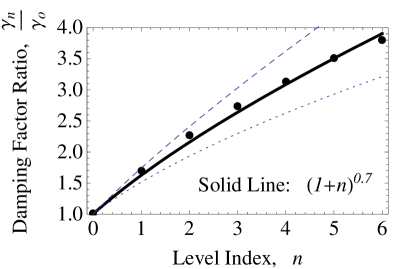
Figure 3: Matching the experimental results for the ratio of damping factors, $\frac{\gamma_{n}}{\gamma_{0}}$. The large dots result from our theoretical calculation of the Born probability using (41) and (44). The solid line is the experimentally measured relation, $(1+n)^{0.7}$. To indicate a scale for the exponent, the thin dashed line is a plot of $(1+n)^{0.8}$, and the thin dotted line is a plot of $(1+n)^{0.6}$.

Figure 3 shows a very good quantitative agreement with experiment (46). Our study indicates that the decoherence measured in meekhof_rabi_1996 is explained simply by the environmental interference characterized in Section VI.2 and having a characteristic frequency of $\approx 5\Omega_{0}$.

In the standard decoherence program, one typically treats these experiments using the decoherence master equation, and ignores the possibility that different ensemble members may suffer environmental interference differently. The generic solution of the master equation describing a system undergoing Rabi oscillations petruccione_open_quantum_systems predicts a constant $\gamma$, with no dependence on $\Omega$. This is one reason why the measured results have been puzzling.

When assuming that all ensemble members suffer interference identically, one has not needed to consider the kinematics associated with indistinguishability. As a consequence, one has searched for dynamical explanations for the measured dependence of $\gamma$ on $\Omega$. For example, for the experiment on Be ions meekhof_rabi_1996 , one has required models with detailed interaction terms exclusive to the experiment itself. Among other things murao_decoherence_1998 ; bonifacio_pra_2000 ; difidio_damped_2000 , one has assumed laser amplitude noise schneider_decoherence_1998 , decay from intermediate levels and, simultaneously, charge-coupling of the ion with the trap’s electrodes budini_localization_2002 ; budini_dissipation_2003 , or feedback damping from polarized background gas polarized by the oscillating ions themselves serra_decoherence_2001 . While plausible, none of these studies has resulted in an agreement as quantitatively good as that in Figure 3.

Because they contain dynamics exclusive to experiments on ions in a Paul trap, many of these models have in effect been tuned to that experiment. They are thus not applicable to the other types of experiments petta_coherent_2005 ; cole_nature_2001 ; zrenner_nature_2002 ; wang_macdonald_prb_2005 ; ramsay_prl_2010 . The models romito_decoherence_2007 ; wang_macdonald_prb_2005 ; ramsay_prl_2010 ; mogilevtsev_prl_2008 used to explain the EID measured in experiments with shallow donors and quantum dots have typically assumed a feedback dynamics from, for example, excitation induced phonons in substrates, and these models have often been quantitatively successful.

When one invokes dynamics to explain a kinematic effect, of course, one risks overly tuning models and misdiagnosing the underlying physics. We have demonstrated that none of these dynamical mechanisms is necessary to explain Excitation Induced Dephasing. As shown in Appendix B, an analogous model for distinguishable ensemble members predicts no dependence of $\gamma$ on $\Omega$. We therefore conclude that a dependence of $\gamma$ on $\Omega$, or EID, may indeed be general, as suggested by experiment, and that it may be a kinematic effect of the indistinguishability of separate, uncontrolled interactions between quantum systems and their environment.

VII Conclusion

In addition to the typical reduced dynamics for open quantum systems petruccione_open_quantum_systems , to understand environmental interference one must faithfully represent the physics involved in the preparation, evolution, and measurement of all members of the experimental ensemble. This means one must address the possibility that different subsets of the experimental ensemble may suffer environmental interference differently.

We have introduced a framework to treat multiple quantum environments. We have discussed a kinematic effect of indistinguishability that affects only open quantum systems. The indistinguishability of experimental ensemble members greatly complicates the partitioning that our approach requires. Based on the beam splitter model, we have made the simplifying hypothesis that environmental interference occurs in events that are themselves indistinguishable. We have not yet investigated alternative treatments, but the kinematic nature of the effect would seem to preclude the possibility of treating it dynamically through a single, “effective” environmental system and a typical reduced dynamics.

To demonstrate our generalization for multiple quantum environments, within the framework we have described two simple systems. We calculated correlation functions for photons scattered at a beam splitter, with and without losses. We created a decoherence model for systems undergoing Rabi oscillations. In one case meekhof_rabi_1996 , we have found unprecedented quantitative agreement with measurements. We have also discovered that the kinematic effect of indistinguishability can explain the generally measured Excitation Induced Dephasing that has previously required different dynamical explanations for different experiments. Full treatment of experiments will likely require more detailed models addressing multiple sources of environmental interference, dressed states, reduced dynamics, etc. But the qualitative and quantitative success of our single, general model for different types of Rabi oscillations experiments is very promising.

Appendix A Including kinematics directly for photon scattering

Here we treat photon scattering as an open system and directly include the kinematics of indistinguishability for a fixed value of $n$. This corresponds to partitioning an ensemble of an arbitrary number of single photons into an ensemble of an arbitrary number of $n$-photon objects.

Let $\rho_{A,n}$ represent the state of the $n$ actively prepared, incident photons. The density operator $\rho_{A,n}$ is defined in the tensor product space $\Phi_{A}^{\otimes n}$, which is spanned by the ket $|i\rangle_{1}|i\rangle_{2}\ldots|i\rangle_{n}\equiv|i_{1}i_{2}\ldots i_{n}\rangle$. The operator $\rho_{A,n}$ therefore remains trivial even when $n$ photons are incident.

The beam splitter passively prepares every member of the experimental ensemble to be in a state represented by $\rho_{B,n}$, which is defined in the tensor product space $\Phi_{B}^{\otimes n}$. Again we will ignore entanglement, so $\rho_{B,n}$ is a sum of projection operators into each of the $2^{n}$ one-dimensional subspaces of $\Phi_{B}^{\otimes n}$. Each projection operator is weighted by $R^{n_{R}}T^{n_{T}}$, where $n_{R}$ and $n_{T}$ are the numbers of reflected and transmitted photons, respectively, represented by the associated one-dimensional subspace.

Consider, for example, the case where $n=3$. One writes the properly symmetrized density operator, $\rho_{B,3}$, to be used on the right hand side of (12), as

$$\rho_{B,3} = R^{3}|rrr\rangle\langle rrr|$$ (51)

$$+R^{2}T\Big{(}|rrt\rangle\langle rrt|+|rtr\rangle\langle rtr|+|trr\rangle\langle trr|\Big{)}$$

$$+RT^{2}\Big{(}|rtt\rangle\langle rtt|+|trt\rangle\langle trt|+|ttr\rangle\langle ttr|\Big{)}$$

$$+T^{3}|ttt\rangle\langle ttt|.$$

If $R+T=1$, then $\mathrm{Tr}\rho_{B,n}=1$ for all $n$.

In the same basis, it is straightforward to construct operators corresponding to the correlation functions calculated in Section V.1. For example,

$$\hat{n}_{R} = 3\,|rrr\rangle\langle rrr|$$ (52)

$$+2\Big{(}|rrt\rangle\langle rrt|+|rtr\rangle\langle rtr|+|trr\rangle\langle trr|\Big{)}$$

$$+1\Big{(}|rtt\rangle\langle rtt|+|trt\rangle\langle trt|+|ttr\rangle\langle ttr|\Big{)}.$$

Proceeding in this fashion, one can reproduce (V.1) for $n=3$.

Appendix B The Rabi oscillations model for distinguishable objects

Here we develop a model based on (5) but for distinguishable ensemble members and interference events. Our scenario is as follows:

1. The members of the ensemble can again suffer environmental interactions at the times $n\Delta\tilde{t}$, where $n=1,2,3\ldots$

2. At every $n\Delta\tilde{t}$, there is some probability, $(1-\eta$), for a member to suffer perturbation and thereby to be prepared passively.

We have again used $\Delta\tilde{t}$ for the timescale of interference. But now we have used the parameter, $\eta$, with $0\leq\eta\leq 1$, to represent the susceptibility of ensemble members to environmental interference. The parameter $\eta$ is the probability for any given member of the ensemble not to suffer interference at one of the times $n\Delta\tilde{t}$. For a perfectly isolated system, $\eta=1$.

We will again assume that passive measurements are fair measurements, and we will not assume any reduced dynamics. We can then write a general formula for the Born probability as more and more branches form:

$$\mathcal{P}_{|g\rangle\langle g|}\big{(}\rho(\tilde{t})\big{)}=\begin{cases}p_{0}(\tilde{t})&0\leq\tilde{t}<1\,\Delta\tilde{t}\\ p_{1}(\tilde{t})&1\,\Delta\tilde{t}\leq\tilde{t}<2\,\Delta\tilde{t}\\ \quad\vdots&\qquad\vdots\\ p_{n}(\tilde{t})&n\Delta\tilde{t}\leq\tilde{t}<(n+1)\Delta\tilde{t}\end{cases}$$ (53)

Here, every $p_{n}(\tilde{t})$ will have the form of the sum in (37), and $M_{branch}=n$.

If members are actively prepared to be in the excited state, and because none will have suffered environmental interference before $\tilde{t}=1\,\Delta\tilde{t}$, we have for the initial value $p_{0}(\tilde{t})=\textrm{sin}^{2}(\Omega\tilde{t})$. It is straightforward to find from the theory of Rabi oscillations

$$p_{1}(\tilde{t})=\eta\,p_{0}(\tilde{t})+(1-\eta)\Big{(}p_{0}(1\Delta\tilde{t})\,\textrm{cos}^{2}\big{(}\Omega\,(\tilde{t}-1\Delta\tilde{t})\big{)}+\big{(}1-p_{0}(1\Delta\tilde{t})\big{)}\,\textrm{sin}^{2}\big{(}\Omega\,(\tilde{t}-1\Delta\tilde{t})\big{)}\Big{)}.$$ (54)

For general $n$, we have

$$p_{n}(\tilde{t})=\eta\,p_{n-1}(\tilde{t})+(1-\eta)\Big{(}p_{n-1}(n\Delta\tilde{t})\,\textrm{cos}^{2}\big{(}\Omega\,(\tilde{t}-n\Delta\tilde{t})\big{)}+\big{(}1-p_{n-1}(n\Delta\tilde{t})\big{)}\,\textrm{sin}^{2}\big{(}\Omega\,(\tilde{t}-n\Delta\tilde{t})\big{)}\Big{)}.$$ (55)

Note the reappearance of a recursive structure similar to that of (41). Recursively partitioning the experimental ensemble in this way (55), however, requires that one can at any time label different ensemble members and know to which partition they belong. Because the recursion index, $n$, is also the index counting time in functions of $n\Delta\tilde{t}$, there is no need to rescale the time parameter, as was done in (43).

Figure 4 shows the results of two sample calculations using (53) with (55).

(a) With $\eta=0.99$, we fit $\gamma/\Omega=0.05$.

(b) With $\eta=0.997$, we fit $\gamma/\Omega=0.015$.

Figure 4: The Born probability, $\mathcal{P}_{|g\rangle\langle g|}\big{(}\rho(\tilde{t})\big{)}$, when members of the ensemble are distinguishable. For both plots, $\Omega\Delta\tilde{t}\approx 0.08$. The dots are the results of recursive calculations using (55) and (53). The solid lines are plots of the damped sinusoid (35) that fits the experimental data. Recall that $\eta$ is the probability that members will not suffer a perturbation at the times $n\Delta\tilde{t}$.

The dots are calculated from our model. The solid lines are plots of the decaying sinusoid in (35), which fits the experimental measurements. For both figures we have used $\Omega\Delta\tilde{t}\approx 0.08$. The results in Figure 4(a) were calculated using $\eta=0.99$ and resulted in a fitted value for the damping factor of $\gamma/\Omega=0.05$. The results in Figure 4(b) were calculated using $\eta=0.997$ and resulted in a fitted value for the damping factor of $\gamma/\Omega=0.015$. Recall that $\eta=1$ for a perfectly isolated system.

This calculation for distinguishable members results in a fitted damping factor, $\gamma$, that is independent of $\Omega$.

References

- (1) P. A. M. Dirac, The Principles of Quantum Mechanics, 4th ed. (Oxford University Press, 1958)
- (2) H. Breuer and F. Petruccione, The Theory of Open Quantum Systems (Oxford University Press, 2002)
- (3) D. M. Meekhof, C. Monroe, B. E. King, W. M. Itano, and D. J. Wineland, Phys. Rev. Lett. 76, 1796 (Mar. 1996)
- (4) W. Nagourney, J. Sandberg, and H. Dehmelt, Phys. Rev. Lett. 56, 2797 (Jun. 1986)
- (5) J. C. Bergquist, R. G. Hulet, W. M. Itano, and D. J. Wineland, Phys. Rev. Lett. 57, 1699 (Oct 1986)
- (6) T. Sauter, W. Neuhauser, R. Blatt, and P. E. Toschek, Phys. Rev. Lett. 57, 1696 (Oct 1986)
- (7) E. Peik, G. Hollemann, and H. Walther, Phys. Rev. A 49, 402 (Jan 1994)
- (8) M. Brune, F. Schmidt-Kaler, A. Maali, J. Dreyer, E. Hagley, J. M. Raimond, and S. Haroche, Phys. Rev. Lett. 76, 1800 (Mar. 1996)
- (9) D. J. Wineland, C. Monroe, W. M. Itano, D. Leibfried, B. E. King, and D. M. Meekhof, J. Res. Natl. Inst. Stand. Technol. 103, 259 (Jun. 1998)
- (10) A. Leggett, in Time’s arrows today: recent physical and philosophical work on the direction of time, edited by S. F. Savitt (Cambridge University Press, 1997)
- (11) I. O. Stamatescu, in Compendium of Quantum Physics, edited by D. Greenberger, K. Hentschel, and F. Weinert (Springer, 2009) pp. 813–822
- (12) R. H. Dicke, Phys. Rev. 93, 99 (1954)
- (13) J. Kempe, D. Bacon, D. Lidar, and K. Whaley, Phys. Rev. A 63, 042307 (Mar. 2001)
- (14) M. Büttiker, Phys. Rev. B 46, 12485 (1992)
- (15) R. Loudon, in Disorder in Condensed Matter Physics, edited by J. Blackman and J. Tagüeña (Clarendon Press, Oxford, 1991) p. 441
- (16) C. C. Gerry and P. L. Knight, Introductory quantum optics (Cambridge University Press, 2005)
- (17) J. N. Dodd, Atoms and Light: Interactions (Plenum Press, New York, 1991) ISBN 0306437414
- (18) J. R. Petta, A. C. Johnson, J. M. Taylor, E. A. Laird, A. Yacoby, M. D. Lukin, C. M. Marcus, M. P. Hanson, and A. C. Gossard, Science 309, 2180 (Sep. 2005)
- (19) B. E. Cole, J. B. Williams, B. T. King, M. S. Sherwin, and C. R. Stanley, Nature 410, 60 (Mar. 2001)
- (20) A. Zrenner, E. Beham, S. Stufler, F. Findeis, M. Bichler, and G. Abstreiter, Nature 418, 612 (2002)
- (21) Q. Q. Wang, A. Muller, P. Bianucci, E. Rossi, Q. K. Xue, T. Takagahara, C. Piermarocchi, A. H. MacDonald, and C. K. Shih, Phys. Rev. B 72, 035306 (Jul. 2005)
- (22) A. J. Ramsay, A. V. Gopal, E. M. Gauger, A. Nazir, B. W. Lovett, A. M. Fox, and M. S. Skolnick, Phys. Rev. Lett. 104, 017402 (2010)
- (23) M. Murao and P. L. Knight, Phys. Rev. A 58, 663 (1998)
- (24) R. Bonifacio, S. Olivares, P. Tombesi, and D. Vitali, Phys. Rev. A 61, 053802 (Apr. 2000)
- (25) C. Di Fidio and W. Vogel, Phys. Rev. A 62, 031802(R) (2000)
- (26) S. Schneider and G. J. Milburn, Phys. Rev. A 57, 3748 (1998)
- (27) A. A. Budini, R. L. de Matos Filho, and N. Zagury, Phys. Rev. A 65, 041402(R) (Apr. 2002)
- (28) A. A. Budini, R. L. de Matos Filho, and N. Zagury, Phys. Rev. A 67, 033815 (Mar. 2003)
- (29) R. M. Serra, N. G. de Almeida, W. B. da Costa, and M. H. Y. Moussa, Phys. Rev. A 64, 033419 (2001)
- (30) A. Romito and Y. Gefen, Phys. Rev. B 76, 195318 (Nov. 2007)
- (31) D. Mogilevtsev, A. P. Nisovtsev, S. Kilin, S. B. Cavalcanti, H. S. Brandi, and L. E. Oliveira, Phys. Rev. Lett. 100, 017401 (2008)