Super Fast and Quality Azimuth Disambiguation
Solar Physics

Abstract

The paper presents the possibility of fast and quality azimuth disambiguation of vector magnetogram data regardless of location on the solar disc. The new Super Fast and Quality (SFQ) code of disambiguation is tried out on well-known models of Metcalf2, Leka1 and an artificial model based on observed magnetic field in AR 10930 [Rudenko et al. (2010)]. We make comparison of Hinode SOT SP vector magnetograms of AR 10930 disambiguated with three codes: SFQ, NPFC [], and SME [Rudenko et al. (2010)]. We illustrate the SFQ disambiguation on SDO/HMI full disk magnetic field observations. The preliminary examination indicates that the SFQ algorithm provides better quality than NPFC and is comparable to SME. In contrast to other codes, SFQ supports relatively high quality which does not depend on the distance to the limb (unlike all other algorithms the presented one remain efficient even when the magnetigram position is very close to the limb).

1 Introduction

Azimuth disambiguation of the transverse field in vector magnetograph data is a key problem determining reliability of the physical researches utilizing the knowledge of full vector of the photospheric magnetic field. Apparently complete and exact solution to this problem is hardly possible because of high level of noise in transverse field data and impossibility of spatial resolution of real pattern of the magnetic field (whose thin structure is significantly less than the spatial resolution of modern magnetographs). In this connection, the main requirement for algorithms of the azimuth disambiguation is to reach invariably high quality that could describe adequately (with minimum distortions) the physically significant real structural elements of magnetic configurations. Also of importance is the code efficiency with regions regardless of their location on the solar disc; this allows us to use data on all available measurements, including those near the limb. To perform on-line processing of continuously incoming data, the final preparation time should be comparable to time of measurement data acquisition. Currently, the best codes providing invariably high quality and meeting the requirements for physical investigation are the codes based on the simulated annealing algorithm (different variants of the "minimum energy" method (ME Metcalf1; Leka2, Rudenko). Quality of the code outcome is significantly higher than the results of other the results available numerous codes [missing (missing)]. Unfortunately, ME codes are among the most long-term: the required time goes up with increasing number of nodes of data grid. Therefore they are not suitable for real-time processing of continuous data flow with high spatial resolution. The SDO/HMI instrument, for instance, generates vector magnetogram with resolution of 4096x4096 once every 12 minutes.

A fast NPFC algorithm [] is now examined in order to be used in data flow processing, since it represents the best compromise between quality and time required for processing. Quality of the NPFC algorithm is ranked second among well-known methods, though it is inferior to that of ME codes. It does not always show invariably satisfactory results in different real configurations of magnetic regions, particularly in those near the limb.

In this paper, we present examples of the azimuth disambiguation of model and real ambiguous magnetograms with the use of three codes: the new Super Fast and Quality (SFQ), NPFC, and SME [Rudenko et al. (2010)]. We show that quality of the SFQ outcome far surpasses that of NPFC. Besides, SFQ is much faster than NPFC. Moreover, time for the azimuth disambiguation of vector-magnetograph data with any spatial resolution (including SDO/HMI measurements of the full disc) may be significantly reduced due to the SFQ parallelization into several processes. This suggests potential on-line processing of current data flow.

2 The method

The SFQ method is a two-step processing system. Step 1 involves preliminary azimuth disambiguation, using special metric (grid difference metric) relying on reference information of the potential field. Step 2 (cleaning) comprises application of smoothing masks in several scales. Our solution does not use random search (like in ME) or convergent iterations (like in NPFC) that’s why it is very fast.

2.1 Step 1

The key point of the method is application of the "grid difference metric" defining measure of difference between the initial ambiguous field ${\bf B}^{amb}$ and the potential (reference) field ${\bf B}^{ref}$. Metric is constructed for each node $I$, $j$ of the magnetogram grid as follows:

$$g^{ij}\left({\bf B}_{\perp}^{amb}\right)=\sqrt{\sum_{s=0}^{1}\sum_{t=0}^{1}\left[\Delta_{s}\left(B_{t}^{amb}-B_{t}^{ref}\right)\right]^{2}};$$

$$\Delta_{0}=f=f^{i+1,j}-f^{i,j},\Delta_{1}=f=f^{i,j}-f^{i,j+1};$$ (1)

$$B_{0}=B_{x},B_{1}=B_{y}.$$

Metric (2.1) is then used as a conditional mask to determine common sign for transverse components of the preliminary field $B^{Step\_1}$:

$$\left({\bf B}_{\perp}^{Step\_1}\right)^{i,j}=\left\{\begin{array}[]{c}\left({\bf B}_{\perp}^{amb}\right)^{i,j}\\ -\left({\bf B}_{\perp}^{amb}\right)^{i,j}\\ \end{array}\right|\left.\begin{array}[]{c}if\quad g^{i,j}\left({\bf B}_{\perp}^{amb}\right)\leq g^{i,j}\left(-{\bf B}_{\perp}^{amb}\right)\\ if\quad g^{i,j}\left({\bf B}_{\perp}^{amb}\right)>g^{i,j}\left(-{\bf B}_{\perp}^{amb}\right)\\ \end{array}\right\}$$ (2)

According to definition of metric (2.1), its application is valid only for nodes with locally continuous ${\bf B}^{amb}$ (i.e., random distribution over azimuth direction nodes fails for ${\bf B}^{amb}_{\perp}$). Consequently, requirement that initial distribution of the transverse field be locally continuous in most nodes is a necessary condition. This requirement is easily satisfied, for instance, if a component of the transverse field ($x$ or $y$) is assumed to be everywhere positive. The potential reference field can be obtained using the standard method for the FFT extrapolation over the longitudinal component $B_{z}$. In our case, we used the potential extrapolation in quasi-spherical geometry [Rudenko et al. (2010)] and subsequent extrapolation of the field into nodes of the initial magnetogram grid.

We think that the principle of construction of metric $g$ (2.1) is similar to the metric used in the most effective ME method:

$$E=\left|j_{z}\right|+\left|\nabla_{\perp}\cdot{\bf B}+\partial_{z}B^{pot}_{z}\right|\equiv\left|j_{z}-j^{pot}_{z}\right|+\left|\nabla_{\perp}\cdot{\bf B}-\nabla_{\perp}\cdot{\bf B}^{pot}\right|$$ (3)

Indeed, close inspection of the equation shows that, formally, terms in the right part of identity (3) are the particular linear combinations of differences (2.1). For simplicity of comparison, we will confine ourselves to the case of flat approximation and $B_{l}=B_{z}$. We attach certain physical meaning to summands of (3). The first summand in (3) provides minimisation of vertical current. This term is responsible for nodes in which local continuity of the transverse ambiguous field is disturbed. In other nodes, it does not depend on azimuth direction of the transverse field. The second summand in (3) is the divergence simulation; it reflects correlation of some differences between the test and reference fields (i.e., it performs function analogous to (2.1). It is thus reasonable to suppose that the main positive function of the azimuth selection in both cases is performed by differential relations between the test and reference fields. We do not assign value of a geometric object’s element (similar to the value of field derivatives making up tensor components of vector field derivatives) to each difference $\Delta_{s}f$ in (2.1). We consider these differences as formal functions of two near points, reflecting local coupling between the test and reference fields. This approach allows us to consider all magnetogram nodes as equivalent (regardless of their location in the visible part of the photosphere) and relieves us of having to use additional grids and geometric transformations. Notice that the NPFC method (which is referred to as nonpotential) uses approximation $\frac{\partial B_{z}}{\partial z}=\frac{\partial B_{z}^{pot}}{\partial z}$ [Metcalf et al. (2006)] when deducing equations for current component $B_{c}$ in indirect form. This condition implies differential reference relation with the potential field.

2.2 Step 2

The necessity to clean the preliminary magnetogram after Step 1 is caused by the peculiar features of our application of metric (2.1). Let us suppose that we apply Step 1 to a noise-free magnetogram of the potential field. In this case, we would probably observe the following: solution to the disambiguation problem is rigorous in the main continuum of points in whose vicinities initial distribution of the transverse field is continuous. Random chains of isolated contrast (bad) pixels on transverse component images would be observed only on lines of the local discontinuity of data. Almost all these bad pixels may be cleaned at one go through comparing with the smoothed transverse field $\overline{{\bf B}}_{\perp}$:

$$\left({\bf B}_{\perp}^{n+1}\right)^{i,j}=\left\{\left.\begin{array}[]{c}\left({\bf B}_{\perp}^{n}\right)^{i,j}\\ -\left({\bf B}_{\perp}^{n}\right)^{i,j}\\ \end{array}\right.\left|\begin{array}[]{c}if\quad\left({\bf B}_{\perp}^{n}\cdot\overline{{\bf B}}_{\perp}^{n}\right)^{i,j}\leq 0\\ if\quad\left({\bf B}_{\perp}^{n}\cdot\overline{{\bf B}}_{\perp}^{n}\right)^{i,j}>0\\ \end{array}\right.\right\}$$ (4)

Typical distribution of bad pixels after Step 1 processing of real magnetograms is well exemplified by images of transverse components $(B_{x},B_{y})$ of Hinode/SOT SP data (Level 2) in the magnetic region AR10930 for two its locations - near the disc centre (Fig. 1) and near the limb (Fig. 2).

Figures show that the general pattern of the transverse field is satisfactorily neat already after Step 1 processing regardless of bad pixels; noteworthy is the fact that the outcome quality near the limb is comparable to that near the centre. This suggests that the chosen metric (2.1) is quite effective, irrespective of proximity to the limb. Close inspection of images in Figures 1 and 2 shows that there are many bad microfragments (groups of adjacent bad pixels). It is obvious that single application of (4) for many of such microfragments may be insufficient. On the other hand, it is reasonable to expect that multiple application of (4), given relevant smoothing parameters, may lead to the "collapse" of fragments due to the motion of their boundaries towards the decrease in absolute magnitude of the transverse field. In practice, most types of bad fragments have the necessary feature: closed fragments, as a rule, collapse (towards the necessary side), whereas open fragments (part of the boundary in the weak noisy field is not seen) transfer their boundaries to the noise region.

We have conducted numerous tests and selected the following type of cleaning (Step 2). Two types of smoothing procedures are used for cleaning. In terms of the IDL code, they have the form:
a) Smoothig(s) - sBx=smooth(Bx,s,$\backslash$edge)-Bx/float(s^2) & sBy=smooth(By,s,$\backslash$edge)-By/float(s^2)
b) Median(s) - sBx=median(Bx,s,$\backslash$even) & sBy=median(Bx,s,$\backslash$even)
Here, $s\times s$ is the size of smoothing window. In this form, smoothing in each node of the grid is performed only in adjacent nodes, exclusive of node values. This modification enhances features of the collapse. Either of smoothing types a) or b) for the chosen parameter $s$ is repeatedly used with subsequent procedure (4) in the cycle with the exit condition: number of iterations reaches 300 or number of modified pixels is less than 5 or 0.01 % of the total amount of pixels.

The final cleaning (Step 2) is the following set of consecutive cycles:
Loop1 - Median(3);
Loop2 - Smoothig(19);
Loop3 - Smoothig(9);
Loop4 - Smoothig(5);
Loop5 - Smoothig(3).
We have used this scheme for all the examples of calculations of model and real magnetograms given before .

3 Model tests

3.1 Known models

To compare SFQ with other codes, we have processed all ambiguous magnetograms of known models used by Metcalf2 and Leka1 to estimate the majority of known methods for the azimuth disambiguation:

• http://www.cora.nwra.com/AMBIGUITY_WORKSHOP/2005/DATA_FILES/Barnes_TPD7.sav

• http://www.cora.nwra.com/AMBIGUITY_WORKSHOP/2005/DATA_FILES/fan_simu_ts56.sav

• http://www.cora.nwra.com/AMBIGUITY_WORKSHOP/2006_workshop/TPD10/TPD10a.sav

• http://www.cora.nwra.com/AMBIGUITY_WORKSHOP/2006_workshop/TPD10/TPD10b.sav

• http://www.cora.nwra.com/AMBIGUITY_WORKSHOP/2006_workshop/TPD10/TPD10c.sav

• http://www.cora.nwra.com/AMBIGUITY_WORKSHOP/2006_workshop/FLOWERS/flowers13a.sav

• http://www.cora.nwra.com/AMBIGUITY_WORKSHOP/2006_workshop/FLOWERS/flowers13b.sav

• http://www.cora.nwra.com/AMBIGUITY_WORKSHOP/2006_workshop/FLOWERS/flowersc.sav

All processing results are presented on http://bdm.iszf.irk.ru/SFQ_Disambig/models.zip by the set of graphs of transverse components of the field (to make a visual estimate) and by the corresponding set of digital IDL sav files ( to make quantitative assessment of vector magnetograms’ quality).

3.2 Answer vector model of AR 10930

The following type of testing of $\pi$-disambiguation methods relies on the answer vector model of the photospheric field of a real magnetic region. Such a model can be easily obtained through fixing vector components of the real component with removed $\pi$-ambiguity (reference magnetogram) by the reference method providing most reliable results. The answer model is the field components of the reference magnetogram transformed into the Carrington spherical coordinate system, with interpolation into nodes of the uniform spherical grid. The resulting field is then used to generate answer magnetograms simulating transit of the selected magnetic configuration across the Sun’s disc. Transforming answer magnetograms into ambiguous ones and comparing their processing effects, we can obtain quantitative assessment for the method under study. Such an approach to modelling allows us to present peculiarities of vector data and features of the real magnetic structure to a great extent in the model. Degree of quality of the quantitative assessment depends on quality of the reference magnetogram. Disambiguation errors in the reference magnetogram affect quality of the following tests. Tests in section 3.1 do not have this disadvantage; on the other hand, there is no assurance that they properly represent real peculiarities of data.

When making the answer vector model in our study, we used vector data on the SOT/SP level 2 (12-17 December 2006) in AR 10930 and the reference SME method of $\pi$ disambiguation [Rudenko et al. (2010)]. Using the model obtained as basis, we simulated transit of a fixed magnetic structure across the disc by a set of answer magnetograms corresponding to moments of AR 10930 real measurement data. To make quantitative assessment, we used standard parameters from Metcalf2 and Leka1:

$$M_{area}=\#pixels(\Delta\theta=0)/\#pixels,\quad\Delta\theta=0^{0}\lor\pm 180^{0};$$

$$M_{flux}=\sum\left(|B_{n}|_{\Delta\theta=0}\right)/\sum|B_{n}|;$$

$$M_{B_{\perp}>T}=\sum(B_{\perp}(s)_{\Delta\theta=0,B_{\perp}>T})/\sum(B_{\perp}(s)_{B_{\perp}>T})$$ (5)

$$M_{\Delta B}=\sum|{\bf B}(s)-{\bf B}(s)|/\#pixels;$$

$$M_{J_{z}}=M(a,s)_{J_{z}}=1-\frac{\sum(J_{n(answer)}-J_{n(solution)})}{2\sum J_{n(answer)}}.$$

Parameter values of $\pi$-disambiguation (3.2) of model magnetograms for three methods (SFQ, SME, and NPFC) are presented is Tables 1-6.

The first and second columns show position of magnetograms on the disc: the first corresponds to the time of real magnetograms with the same position on the disc; the second demonstrates angular distance from the disc centre to the centre of an arbitrarily chosen region. Under close examination, we see that the SFQ quality in these tables is closer to SME. NPFC demonstrates the worst quality near the limb. When approaching the limb, most SFQ parameters seem more preferable than SME. Besides, it is easily seen that the SFQ quality all along the region transit is almost always on the same high level, whereas results of other methods deteriorate to a variable degree when approaching the limb. The last line of the table does not correspond to the time of the real magnetogram. Parameters of this line show the SFQ efficiency in the artificial position of the region when major part of the strong field stricture is behind the limb. Images of transverse components of the answer magnetogram and SFQ magnetogram in this case are presented in Fig. 3 and 4, respectively. This example proves that we can apply the SFQ method for $\pi$ disambiguation of full-disc magnetograms without significant distortions of magnetic structures on the limb.

All other images corresponding to Tables 1-6 are available on:

http://bdm.iszf.irk.ru/SFQ˙Disambig/Answer˙AR10930˙model.zip

– transverse components of answer magnetograms;

http://bdm.iszf.irk.ru/SFQ˙Disambig/SFQ˙AR10930˙model.zip

– transverse components of SFQ magnetograms;

http://bdm.iszf.irk.ru/SFQ˙Disambig/SME˙AR10930˙model.zip

– transverse components of SME magnetograms;

http://bdm.iszf.irk.ru/SFQ˙Disambig/NPFC˙AR10930˙model.zip

– transverse components of NPFC magnetograms

4 Disambiguation of real magnetogram data

4.1 AR 10930

Complete set of graphics files containing results of $\pi$-disambiguation of real Hinode/SOT SP (Level 2) magnetogram data of AR 10930 by three methods is available on:

http://bdm.iszf.irk.ru/SFQ˙Disambig/SFQ˙AR10930.ZIP

– transverse components of SFQ magnetograms;

http://bdm.iszf.irk.ru/SFQ˙Disambig/SME˙AR10930.ZIP

– transverse components of SME magnetograms;

http://bdm.iszf.irk.ru/SFQ˙Disambig/NPFC˙AR10930.ZIP

– transverse components of NPFC magnetograms.

Let us comment on these results, using two cases of the magnetic field location - near the centre (Fig. 5-7) and near the limb (Fig. 8-10).

Fig. 5-7 illustrate similar quality of disambiguation by the three methods. When the magnetic region is at its nearest to the limb (Fig. 8-10), only SFQ code copes with the task successfully. Throughout this series of magnetograms, only SFQ code demonstrates satisfactory quality. SME provides good quality for all magnetograms except for the last one. NPFC maintains satisfactory level of quality from 12 December 2006, 20:30:05 (Lc=50.1348770), to 15 December 2006, 05:45:05 (Lc=50.1348770). Unlike other codes, SFQ maintains stable level of quality regardless of distance to the limb. This is consistent with the quantitative analysis presented in section 3.2.

4.2 disambiguation of full-disc SDO/HMI data

In this subsection, we demonstrate disambiguation of SDO/HMI data obtained 2 July 2010 for the entire disc in original spatial resolution. Initial data were taken from http://sun.stanford.edu/~todd/HMICAL/VectorB/. We divided data into 10x10 rectangular fragments and sequentially applied the SFQ code to them. Fig. 11 presents the result of fragment assembly (file containing this image in full resolution and FITS files of the field components are available on http://bdm.iszf.irk.ru/SFQ_Disambig/20100702_010000_hmi.zip). It takes about one hour to disambiguate with Core 2 Quad (2.6 GHz) workstation. The result that we have obtained demonstrates good quality for all large-scale and small-scale magnetic structures with magnitudes higher than the noise level throughout the disc. Notice that the corrected magnetogram has a patchwork structure in the field of very weak fields. This is due to extremely low signal-to-noise ratio in the regions with very weak fields

5 Conclusion

This paper presents a new code for the azimuth disambiguation of vector magnetograms. Among all well-known algorithms for the azimuth disambiguation, SFQ is the fastest (more than 4 times faster as compared to the NPFC algorithm). Besides, our algorithm provides invariably high quality in all parts of the solar disc. This statement has been proved by testing on well-known analytical models and using real data from HINODE SOT/SP and SDO/HMI instruments. In the case of real magnetograms, the method is efficient near the limb where other algorithms (ME and NPFC) do not give reliable results. Due to the high speed and quality of disambiguation, the SFQ method can be applied to process SDO/HMI vector magnetograms in full resolution (4096x4096) and in almost real-time mode.

All magnetograms presented in the paper are available on http://bdm.iszf.irk.ru/SFQ_Disambig.

Acknowledgements

G. Barnes and NASA/LWS contract NNH05CC75C, K. D. Leka (PI) model data are used here.

This work was supported by the Ministry of Education and Science of Russian Federation (GS 8407 and GK 14.518.11.7047) and by the RFBR (12-02-31746 mol_a)

Table 1.: $M_{area}$

Magnetograms	Lc	SFQ	SME	NPFC
20061212_203005	19.2	0.80	0.93	0.74
20061213_043005	23.5	0.80	0.93	0.74
20061213_075005	25.2	0.80	0.93	0.74
20061213_125104	28.0	0.81	0.91	0.74
20061213_162104	29.8	0.80	0.91	0.75
20061214_002005	34.1	0.81	0.89	0.74
20061214_050005	36.7	0.81	0.88	0.75
20061214_112602	40.3	0.81	0.87	0.74
20061214_140103	41.6	0.80	0.86	0.74
20061214_220005	45.9	0.81	0.84	0.74
20061215_054505	50.1	0.80	0.82	0.74
20061215_130205	54.2	0.80	0.81	0.73
20061215_204604	58.3	0.81	0.79	0.72
20061216_012106	60.8	0.80	0.78	0.72
20061216_075005	64.4	0.80	0.78	0.70
20061216_123104	67.0	0.80	0.78	0.69
20061217_002528	73.1	0.80	0.76	0.56
20061218_032421	87.9	0.76	-	-

Table 2.: $M_{flux}$

Magnetograms	Lc	SFQ	SME	NPFC
20061212_203005	19.2	0.95	0.99	0.95
20061213_043005	23.5	0.95	0.99	0.95
20061213_075005	25.2	0.95	0.99	0.95
20061213_125104	28.0	0.95	0.99	0.96
20061213_162104	29.8	0.95	0.99	0.96
20061214_002005	34.1	0.96	0.99	0.96
20061214_050005	36.7	0.96	0.98	0.96
20061214_112602	40.3	0.96	0.98	0.96
20061214_140103	41.6	0.96	0.98	0.96
20061214_220005	45.9	0.96	0.98	0.96
20061215_054505	50.1	0.96	0.97	0.95
20061215_130205	54.2	0.97	0.97	0.95
20061215_204604	58.3	0.96	0.96	0.94
20061216_012106	60.8	0.97	0.96	0.93
20061216_075005	64.4	0.96	0.96	0.91
20061216_123104	67.0	0.96	0.96	0.90
20061217_002528	73.1	0.96	0.96	0.66
20061218_032421	87.9	0.95	-	-

Table 3.: $M_{B\bot>500G}$

Magnetograms	Lc	SFQ	SME	NPFC
20061212_203005	19.2	0.99	1.00	0.99
20061213_043005	23.5	0.98	1.00	0.99
20061213_075005	25.2	0.98	1.00	0.99
20061213_125104	28.0	0.97	1.00	0.99
20061213_162104	29.8	0.97	1.00	0.99
20061214_002005	34.1	0.97	1.00	0.99
20061214_050005	36.7	0.96	1.00	0.99
20061214_112602	40.3	0.96	1.00	0.99
20061214_140103	41.6	0.96	1.00	0.99
20061214_220005	45.9	0.96	1.00	0.99
20061215_054505	50.1	0.96	1.00	0.99
20061215_130205	54.2	0.97	1.00	0.99
20061215_204604	58.3	0.97	1.00	0.98
20061216_012106	60.8	0.97	1.00	0.98
20061216_075005	64.4	0.96	0.99	0.96
20061216_123104	67.0	0.96	0.99	0.95
20061217_002528	73.1	0.97	0.99	0.61
20061218_032421	87.9	0.95	-	-

Table 4.: $M_{B\bot>100G}$

Magnetograms	Lc	SFQ	SME	NPFC
20061212_203005	19.2	0.96	0.99	0.95
20061213_043005	23.5	0.96	0.99	0.95
20061213_075005	25.2	0.95	0.99	0.95
20061213_125104	28.0	0.96	0.99	0.95
20061213_162104	29.8	0.96	0.99	0.96
20061214_002005	34.1	0.96	0.99	0.96
20061214_050005	36.7	0.96	0.99	0.96
20061214_112602	40.3	0.95	0.99	0.96
20061214_140103	41.6	0.95	0.99	0.96
20061214_220005	45.9	0.96	0.99	0.97
20061215_054505	50.1	0.96	0.99	0.97
20061215_130205	54.2	0.96	0.99	0.96
20061215_204604	58.3	0.96	0.98	0.96
20061216_012106	60.8	0.96	0.98	0.95
20061216_075005	64.4	0.95	0.97	0.93
20061216_123104	67.0	0.95	0.97	0.93
20061217_002528	73.1	0.95	0.96	0.62
20061218_032421	87.9	0.93	-	-

Table 5.: $M_{B\Delta}(G)$

Magnetograms	Lc	SFQ	SME	NPFC
20061212_203005	19.2	28.3	8.1	38.2
20061213_043005	23.5	27.6	8.2	37.4
20061213_075005	25.2	28.4	6.7	38.0
20061213_125104	28.0	25.3	9.3	38.0
20061213_162104	29.8	27.1	8.2	36.2
20061214_002005	34.1	25.8	10.8	36.2
20061214_050005	36.7	24.7	11.9	35.5
20061214_112602	40.3	25.4	13.0	36.3
20061214_140103	41.6	29.1	14.6	36.8
20061214_220005	45.9	25.8	17.0	36.0
20061215_054505	50.1	27.1	19.9	36.6
20061215_130205	54.2	25.6	21.5	36.0
20061215_204604	58.3	27.3	25.0	45.6
20061216_012106	60.8	26.7	27.7	46.2
20061216_075005	64.4	28.6	26.5	62.1
20061216_123104	67.0	29.5	26.9	70.1
20061217_002528	73.1	28.8	29.8	257.8
20061218_032421	87.9	32.6	-	-

Table 6.: $M_{Jz}$

Magnetograms	Lc	SFQ	SME	NPFC
20061212_203005	19.2	0.82	0.95	0.76
20061213_043005	23.5	0.83	0.95	0.76
20061213_075005	25.2	0.83	0.95	0.76
20061213_125104	28.0	0.84	0.94	0.76
20061213_162104	29.8	0.83	0.95	0.77
20061214_002005	34.1	0.83	0.93	0.78
20061214_050005	36.7	0.84	0.92	0.78
20061214_112602	40.3	0.84	0.92	0.78
20061214_140103	41.6	0.82	0.91	0.78
20061214_220005	45.9	0.84	0.90	0.79
20061215_054505	50.1	0.84	0.89	0.79
20061215_130205	54.2	0.85	0.89	0.80
20061215_204604	58.3	0.85	0.88	0.77
20061216_012106	60.8	0.86	0.87	0.77
20061216_075005	64.4	0.86	0.87	0.75
20061216_123104	67.0	0.86	0.87	0.74
20061217_002528	73.1	0.87	0.86	0.55
20061218_032421	87.9	0.90	-	-

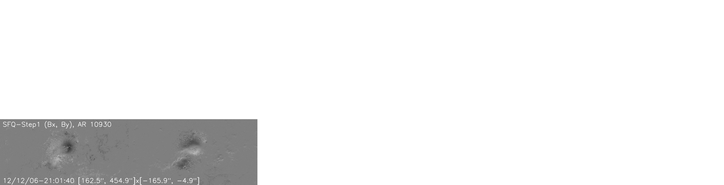
Figure 1.: Transverse components of the magnetic region AR 10930 near the disc centre after Step 1 processing.

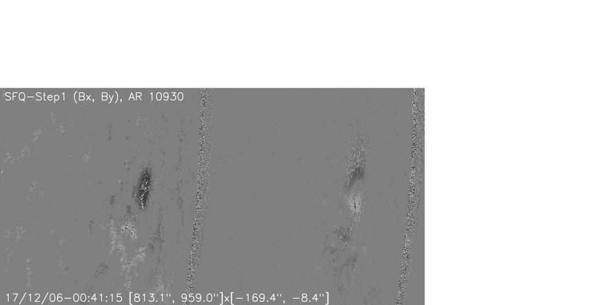
Figure 2.: Transverse components of the magnetic region AR 10930 near the limb after Step 1 processing.

Figure 3.: Limb answer magnetogram of the AR 10930 model. Lc=87.9

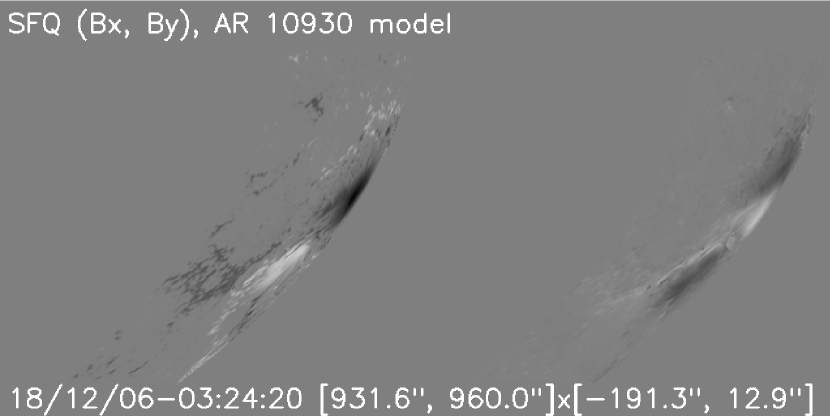
Figure 4.: . Limb SFQ magnetogram of the AR 10930 model. Lc=87.9

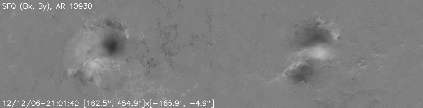
Figure 5.: Near-Centre SFQ magnetogram of AR 10930. Lc=19.2

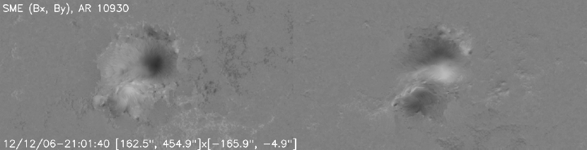
Figure 6.: Near-Centre SME magnetogram of AR 10930. Lc=19.2

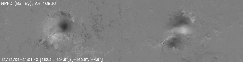
Figure 7.: Near-Centre NPFC magnetogram of AR 10930. Lc=19.2

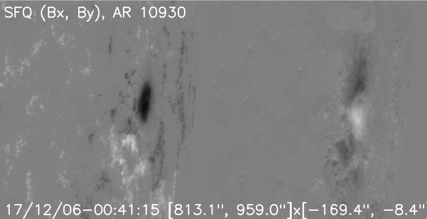
Figure 8.: Near-Limb SFQ magnetogram of AR 10930. Lc=73.1

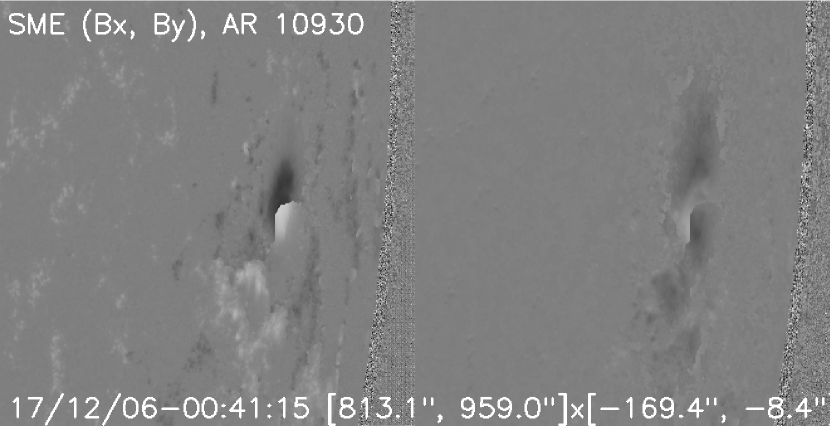
Figure 9.: Near-Limb SME magnetogram of AR 10930. Lc=73.1

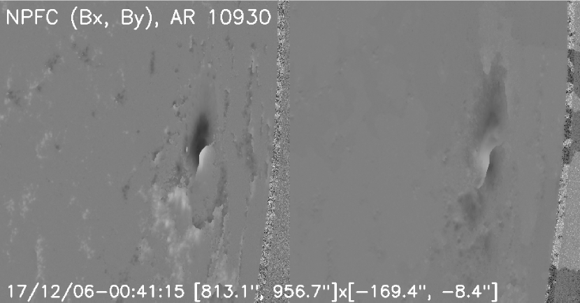
Figure 10.: Near-Limb NPFC magnetogram of AR 10930. Lc=73.1

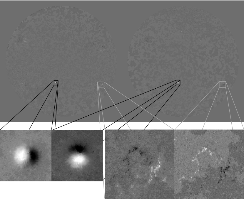
Figure 11.: Full-disc SDO/HMI on 2 July 2010.

References

- [ ] Georgoulis, M. K.: 2005, ApJ 629, L69.
- Leka et al. (2009) Leka, K. D., Barnes, G., Grouch, A. D., Gary, G. A., Jing, J, and Liu, Y.: 2009, Sol. Phys. 260, 83.
- Leka, Barnes and Crouch (2009) Leka, K. D., Barnes, G.; Crouch, A.:2009, The Second Hinode Science Meeting: Beyond Discovery-Toward Understanding ASP Conference Series, Vol. 415, proceedings of a meeting held 29 September through 3 October 2008 at the National Center for Atmospheric Research, Boulder, Colorado, USA. Edited by B. Lites, M. Cheung, T. Magara, J. Mariska, and K. Reeves. San Francisco: Astronomical Society of the Pacific, 2009, p.365
- missing (missing) Metcalf, T. R.: 1994, Sol. Phys. 155, 235.
- Metcalf et al. (2006) Metcalf, T. R., Leka, K. D., Barnes, G., Lites, B. W., Georgoulis, M. K., Pevtsov, A. A, et al.: 2006, Sol. Phys. 237, 267.
- Rudenko et al. (2010) Rudenko, G. V., Myshyakov, I. I., and Anfinogentov, S. A.: 2011, eprint arXiv:1007.0298 (Acsepted in Geomagnetism and Aeronomy)