Observers in an accelerated universe.

Abstract

If the current acceleration of our Universe is due to a cosmological constant, then a Coleman-De Luccia bubble will nucleate in our Universe. In this work, we consider that our observations could be likely in this framework, consisting in two infinite spaces, if a foliation by constant mean curvature hypersurfaces is taken to count the events in the spacetime. Thus, we obtain and study a particular foliation, which covers the existence of most observers in our part of spacetime.

Our Universe is currently undergoing a period of accelerated expansion. If this acceleration is due to a cosmological constant, then our future Universe will be a de Sitter space. Coleman and De Luccia considered that a de Sitter universe could be understood as a false vacuum which would decay into the true vacuum Coleman:1980aw (see also Ref. Coleman:1977py ), leading to the nucleation of a bubble in the original de Sitter space which grows at a velocity close to the speed of light Coleman:1980aw . Despite implying a catastrophic end for part of the original universe, that process was gladly received in the inflationary paradigm, residing at the very basis of Linde’s eternal inflation Linde:1986fc , and it could also lead to interesting future scenarios Garriga:1997ef . Moreover, those Coleman-De Luccia bubbles (CDL) have taken a renewed interest (see, for example, Ref. Yamauchi:2011qq ) in the context of the string theory landscape Susskind:2003kw .

On the other hand, the nucleation of a CDL bubble is not the most surprising phenomenon which could take place in our future Universe. As a de Sitter spacetime last forever, an infinite number of putative observers could form from thermal and/or vacuum fluctuations arbitrarily late (see Page:2008zh references therein); therefore, it could seem that our observations are unlikely. It should be worth noticed that such paradoxical result depends on the assigned measure and, at the end of the day, on how we count the events within the spacetime. As it is well known, general relativity cannot provide us with a preferred foliation by spacelike hypersurface in order to count the number of events within a spacetime. A possible choice is a foliation by hypersurfaces of constant mean curvature (CMC), which can be considered in different spacetimes regardless of the particular symmetry. Furthermore, those foliations provide us with a quantity which can play the role of time York ; Kuchar and they can be used to study different topics from canonical general relativity Barbour:2010xk to numerical relativity Metzger:2004pr . Moreover, Page has pointed out that the foliations by CMC hypersurfaces could also play an essential role regarding a new approach to the measure problem in the framework of eternal inflation Page:2008zh , where the mentioned paradoxical result is also present. It has been suggested that in the case of a de Sitter space with a CDL bubble of de Sitter space inside this foliation might not be enough to cover the existence of most observers in this space. Nevertheless, if that would not be the case and a foliation by CMC hypersurfaces could cover the existence of most observers in our part of spacetime, then that could provide us with at least approximately the right measure for our observations Page:2008zh .

It is the main aim of the present paper considering whether a foliation by CMC hypersurfaces of a de Sitter space with a CDL bubble of de Sitter space inside could cover the existence of most observers in our region of spacetime. It should be emphasized that this spacetime consists of two infinite spacetimes. Therefore, if a CMC foliation covers most of the spacetime, then it can be used, by taking a certain measure, to get at least approximately the right probability to the occurrence of the events. That could also be done even in the case that the foliation may not penetrate significantly in the inside space, if one assumes that the main contribution to obtain the probabilities would come from our spacetime region Page:2008zh . Nevertheless, if the foliation would not be enough to cover our existence, then choosing such a foliation would imply that our observations are extremely unlikely, being more natural putative observers measures. As that would be an uncomfortable result, in that case we should discard the use of CMC foliations.

First of all, the spacetime must be regular; therefore, the Israel junction conditions Israel:1966rt must be fulfilled on the bubble wall. The trajectory of the wall can be obtained easily considering the coordinates in the 5-dimensional Minkowski space, where a de Sitter spacetime can be visualized as the hyperboloid HyE

$$-v^{2}+w^{2}+(x^{i})^{2}=\alpha^{2},$$ (1)

with $\alpha=\sqrt{3/\Lambda}$ and $\Lambda$ is the cosmological constant. Due to the high level of symmetry of this space, one can introduce different charts of coordinates in the hyperboloid expressing the metric by different $3+1$ decompositions. These are given by

$${\rm d}s^{2}=-{\rm d}t^{2}+a(t)^{2}\left[{\rm d}\eta^{2}+f\left(\eta\right)^{2}\,{\rm d}\Omega_{(2)}^{2}\right],$$ (2)

where ${\rm d}\Omega_{(2)}^{2}={\rm d}\theta^{2}+\sin^{2}\theta{\rm d}\phi^{2}$, with $0\leq\theta\leq\pi,\,0\leq\phi\leq 2\pi$. The closed slicing, given by $a(t)=\alpha\,{\rm cosh}\left(t/\alpha\right)$ and $f\left(\eta\right)=\sin\eta$, with $-\infty<t<\infty$ and $0\leq\eta\leq\pi$, covers the whole hyperboloid and leads to the Carter-Penrose (C-P) diagram through $T=2\,{\rm arctan}\left[{\rm exp}\left(t/\alpha\right)\right]-\pi/2$. The functions $a(\hat{t})=\exp\left(\hat{t}/\alpha\right)$ and $f\left(\hat{\eta}\right)=\hat{\eta}$ correspond to the flat slicing with $-\infty<\hat{t}<\infty$ and $0\leq\hat{\eta}$. The open slicing is given by $a(\tau)=\alpha\,{\rm sinh}\left(\tau/\alpha\right)$, $f\left(\chi\right)={\rm sinh}\chi$, $\tau\geq 0$ and $\chi<\infty$. We consider, without lost of generality, that the bubble nucleates at $t=0$ and that it is centered at $\eta=0$, where the coordinates of the closed slicing have been taken. Therefore, following a similar procedure to that considered in Ref. Garriga:1997ef for the flat slicing, the trajectory of the wall in the outside space can be given by fixing $w^{*}=D$. Therefore, this trajectory can be expressed as

$$\eta^{*}(t)={\rm arccos}\left[\frac{D}{\alpha\cosh(t/\alpha)}\right],$$ (3)

where ^∗ means evaluation on the wall. As it can be seen from condition (1) and the relation between the coordinates of the hyperboloid and those of the closed slicing HyE , we have $D<\alpha$ for $D>0$, implying that the trajectory is well-defined. Therefore, the outside region can be described by the closed slicing with $\eta^{*}\leq\eta\leq\pi$. The bubble wall tends to $\pi/2$ when $t\rightarrow\infty$, see Fig. 1. A bubble which nucleates with the minimal possible size, $D/\alpha\rightarrow 1$, will expand with maximal velocity; although it must be noticed that the case $D=\alpha$ cannot be properly studied by using the thin-wall approximation. Considering decay models leading to smaller values of this quotient, one obtains bubbles with bigger initial sizes, tending the trajectories of their walls to that of the smallest bubble for large values of $T$.

Figure 1: Trajectory of the wall for different decay models corresponding to values of $D/\alpha$ in the interval $[1,0.1]$, from the left to the right. The C-P diagram of the outside space is the same as that of the de Sitter universe removing the region on the left of the bubble wall from the moment that it nucleates, $T=0$. A similar figure can be obtained considering the inside space, corresponding the diagram to the region bounded by $0<T_{b}<\pi/2$ and $0\leq\eta_{b}\leq\eta_{b}^{*}$.

The first junction condition, ${\rm d}s^{2}|_{{\rm wall}}={\rm d}s_{b}^{2}|_{{\rm wall}}$ (where the subscript $b$ denotes the quantities related to the inside space), can also be imposed in the 5-dimensional space more easily than in the 4-dimensional one. It leads to a trajectory of the wall in the inside space which takes a similar form to that of the outside space, Eq. (3), with

$$D_{b}^{2}=D^{2}+\alpha_{b}^{2}-\alpha^{2},$$ (4)

and to the following equation

$$\sinh(t_{b}/\alpha_{b})=\alpha/\alpha_{b}\sinh(t/\alpha),$$ (5)

which must be fulfilled on the wall. Therefore, as seen from the inside space, the bubble contains a region bigger than the future light cone of its center (see Figs. 1). It must be worth noticed that this light cone contains an infinite universe inside when the open slicing is considered Gott:1982zf ; Bucher:1994gb .

The second junction condition relates the value of the difference of the extrinsic curvatures of both regions on the wall to the surface density of the energy-momentum tensor on the wall Berezin . Therefore, the particular value of $D$ depends on the value of both cosmological constants and on the particular form of the potential which presents the two minima Parke:1982pm . The fulfillment of this junction condition has led to some controversy about the possible decay of a true vacuum into a false vacuum Lee:1987qc , since a false vacuum bubble able to grow indefinitely must necessarily have emerged from an initial singularity if the null energy condition is satisfied Farhi:1986ty . Nevertheless, the consideration of some scenarios Ansoldi:2007fw ; Lee:2007dh would lead to the possible existence of unbounded false vacuum bubbles. Therefore, we will impose no restriction on the relation between both energies, in order to maintain our analysis as general as possible.

On the other hand, there are a number of known properties of CMC hypersurfaces in cosmological spacetimes satisfying the strong energy condition Marsden . Nevertheless, if the strong energy condition is violated, as it occurs in a de Sitter space with or without CDL bubble, then even less results are available (see Ref. Beig:2005ef and references therein for information about developments in this particular field, and Ref. Malec:2009hg for recent studies considering different spacetimes). Nevertheless, we can notice that the hypersurfaces with CMC in a de Sitter space with a thin-wall CDL bubble of de Sitter space inside would also have CMC in a simple de Sitter space. The closed slicing of a de Sitter space provides us with a simple CMC foliation which covers the whole space, that is the constant cosmic time foliation. But the foliation by hypersurfaces with constant $t$ in the outside region and with constant $t_{b}$ inside the bubble is not a CMC foliation. Therefore, in order to find a CMC foliation of the considered space, in the first place, we should solve the differential equation implied by $K={\rm constant}$. However, it can be seen that this is a non-trivial differential equation.

Let us reflect on the symmetry of the problem to find particular solutions to the differential equation. A de Sitter hyperboloid is a CMC 4-hypersurface in the 5-dimensional Minkowski space. Thus, one could think that the intersection of two 4-hypersurfaces with CMC in a 5-dimensional Minkowski space produces a 3-hypersurface which would also have CMC, when considering this hypersurface defined in the spacetime given by one of the original 4-hypersurfaces. Thus, taking this argument and the symmetry of the problem into account, one can consider the simplest 4-dimensional hypersurfaces with CMC in a Minkowski space; those are the hyperplanes which can be seen as lines in a $(v,\,w)$-section of the space, i. e. $\Sigma_{4}:\,\,v=b\,w+a,$ where $b$ and $a$ are arbitrary constants, which describe the slope and the $v$-intercept, respectively. It must be worth noticed that, in the 5-dimensional Minkowski space, the hyperplanes are related by boots with those 4-hypersurfaces which lead to the constant cosmic time foliation of the closed slicing when they intersect the hyperboloid; therefore, they are, of course, CMC in the 5-dimensional space (with $K_{(4)}=0$). Nevertheless, this is not necessarily ensuring that their intersections with the hyperboloid lead to CMC 3-hypersurfaces in the 4-dimensional de Sitter space; that is precisely what we are arguing. Therefore, we must calculate the trace of the extrinsic curvature of the 3-hypersurfaces, $K=K_{(3)}\neq K_{(4)}$, in order to check whether they really have CMC in a de Sitter space. The intersections of the hyperplanes and the hyperboloid lead to the hypersurfaces

$$\cosh(t/\alpha)=\frac{ba\cos\eta+\sqrt{a^{2}+1-b^{2}\cos^{2}\eta}}{1-b^{2}\cos^{2}\eta},$$ (6)

in a de Sitter space; where we have ruled out the solution with a minus sign multiplying the square root, because they must simplify to the correct constant value for $b=0$ (which is the case of the constant $t$ foliation). The trace of the extrinsic curvature of these 3-hypersurfaces is

$$K=-3\frac{a}{\alpha\sqrt{a^{2}+1-b^{2}}},$$ (7)

which is constant for each hypersurface. Thus, these are spherically symmetric CMC hypersurfaces in a de Sitter space.

In the second place, as the previous procedure is valid for any de Sitter space, we consider that the hypersurfaces are given in the inside space by a similar expression. Therefore, the hypersurfaces are CMC throughout the whole space only if $K=K_{b}$, that is

$$\frac{a}{\alpha\sqrt{a^{2}+1-b^{2}}}=\frac{a_{b}}{\alpha_{b}\sqrt{a_{b}^{2}+1-b_{b}^{2}}}.$$ (8)

In the third place, the hypersurfaces must be regular. Therefore, we have to impose: (i) the hypersurfaces must fulfill the first junction condition on the bubble wall, and (ii) the scalar product of the orthonormal vector to the CMC hypersurface and the orthonormal vector to the wall at the intersection of both hypersurfaces must be constant. These conditions imply:

$$bD+a\alpha=b_{b}D_{b}+a_{b}\alpha_{b},$$ (9)

and

$$\frac{a\frac{D}{\alpha}+b}{\sqrt{(1-\frac{D^{2}}{\alpha^{2}})(a^{2}+1-b^{2})}}=\frac{a_{b}\frac{D_{b}}{\alpha_{b}}+b_{b}}{\sqrt{(1-\frac{D_{b}^{2}}{\alpha_{b}^{2}})(a_{b}^{2}+1-b_{b}^{2})}}.$$ (10)

Thus, we have a system of three equations, Eqs. (8), (9) and (10), with four unknown quantities, $\{a,\,b,\,a_{b},\,b_{b}\}$. This system has two sets of solutions, which are

$$a=-b\frac{\alpha}{D},\,\,a_{b}=-b\frac{\alpha_{b}}{D},\,\,b_{b}=b\frac{D_{b}}{D},$$ (11)

and

$$a=-b\frac{\alpha(\alpha^{2}-\alpha_{b}^{2})}{-2\alpha\alpha_{b}D_{b}+D(\alpha^{2}+\alpha_{b}^{2})},{}$$

$${}a_{b}=b\frac{\alpha_{b}(\alpha^{2}-\alpha_{b}^{2})}{-2\alpha\alpha_{b}D_{b}+D(\alpha^{2}+\alpha_{b}^{2})},{}$$

$${}b_{b}=b\frac{D_{b}(\alpha^{2}+\alpha_{b}^{2})-2D\alpha\alpha_{b}}{-2\alpha\alpha_{b}D_{b}+D(\alpha^{2}+\alpha_{b}^{2})}.$$ (12)

Each set of solutions describes a different foliation, being each hypersurface given by a particular value of $b$. Foliation I, Eq. (11), can be studied by using general considerations. Whereas it is not possible to perform a detailed study about foliation II, Eq. (Observers in an accelerated universe.), without restricting to a particular decay model. Nevertheless, it can been noticed, by studying both foliations for the same particular values of the parameters, that foliation II covers a region of the space smaller than that covered by foliation I, at least for those values. Therefore, foliation I and II are not equivalent. It must be emphasized that these foliations are only the foliations coming from a particular kind of CMC hypersurfaces in the 5-dimensional space, the 4-hyperplanes. If the argument which we have included would be valid in general, then it could help us to find more CMC foliations. Moreover, it should be kept in mind that it is also possible, at least in principle, that there would be foliations by CMC hypersurfaces of a de Sitter space which are not produced by a family of CMC 4-hypersurfaces in the 5-dimensional Minkowski space intersecting the hyperboloid.

We can express the hypersurfaces of foliation I in the outside space, taking into account Eqs. (6) and (11), as

$$\cosh\left(t/\alpha\right)=\frac{-b^{2}\cos\eta+\sqrt{b^{2}+\lambda^{2}(1-b^{2}\cos^{2}\eta)}}{\lambda(1-b^{2}\cos^{2}\eta)},$$ (13)

where $\lambda\equiv D/\alpha$, with $0<\lambda<1$. The hypersurfaces are well-defined for $b^{2}\leq 1$. As we are only interested in the no-contracting region, we consider $b\leq 0$ (which corresponds to $K\leq 0$); therefore $-1\leq b\leq 0$. It can be noticed that the hypersurface given by $b=-1$ diverges at $\eta=\pi$, and every hypersurface intersects the wall at a finite $t$. Thus, the foliation covers an infinite region of the outside space, but it also avoids an infinite part. The foliation covers a “larger” region of the space for smaller values of $\lambda$, that is for bubbles nucleated with bigger initial sizes. In Fig. 2 we show the CMC hypersurfaces in the C-P diagram of the outside space for a particular decay model.

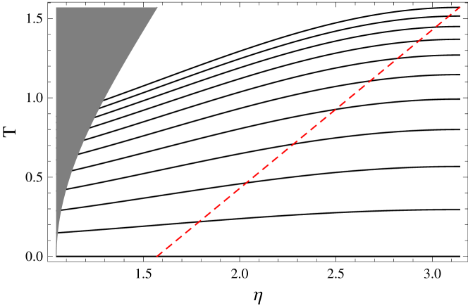
Figure 2: CMC hypersurfaces (continuous lines) in the region $T\geq 0$ of the C-P diagram of the outside space for a model with $\lambda=0.5$. The gray region is not part of this space. The closed slicing covers the whole diagram, whereas the flat slicing only covers the region of this diagram on the left of the dashed line. In this figure the geodesics of the congruence would be vertical straight lines covering the whole diagram.

Those hypersurfaces can be described in the inside region by

$$\cosh\left(t_{b}/\alpha_{b}\right)={}$$

$$\frac{-b^{2}\lambda_{b}\cos\eta_{b}+\beta\sqrt{\beta^{2}+b^{2}(1-\lambda_{b}^{2}\cos^{2}\eta_{b})}}{\beta^{2}-\lambda_{b}^{2}b^{2}\cos^{2}\eta_{b}},$$ (14)

with $\lambda_{b}\equiv D_{b}/\alpha_{b}$, $0<\lambda_{b}<1$, and $\beta\equiv D/\alpha_{b}$. Taking into account Eq. (4), it can be obtained that $0<\beta<\lambda<\lambda_{b}<1$, in the case of a true vacuum bubble (TVB) which nucleates in a false vacuum ($\alpha_{b}>\alpha$); whereas if one considers a false vacuum bubble (FVB, $\alpha_{b}<\alpha$), then $0<\lambda_{b}<\lambda<\beta<\alpha/\alpha_{b}$. These hypersurfaces, with $-1\leq b\leq 0$, are well-defined in the considered range. The foliation only covers a finite region inside the bubble. This covered finite region is larger for smaller values of $\beta$. For values of $\lambda_{b}\rightarrow 1$, the foliation only covers a small region of the inside space; this fact can be understood thinking that in this case the initial size of the bubble is so small that there is almost nothing to cover at $t_{b}=0$, and the bubble grows so quickly that the foliation cannot come into the inside space. For values of $\lambda_{b}\rightarrow 0$, the foliation covers a larger region of the inside space, because this space almost corresponds to the whole causal connected region of the bubble center (see Fig. 1). In Fig. 3 we show the behavior of the CMC hypersurfaces at the end of the foliation ($b=-1$) in the C-P diagram of the inside space for different decay models.

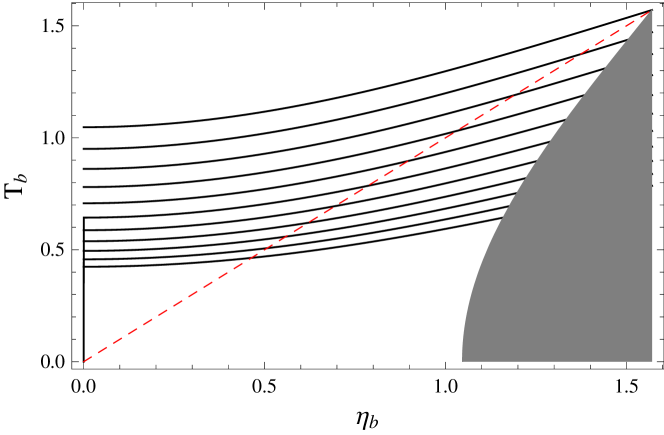
Figure 3: C-P diagram of the inside space for different models with $\lambda_{b}=0.5$ and $\beta$ in the interval $[0,1]$. The gray region is not part of this space. The maximal CMC hypersurfaces (continuous lines) of those models, which corresponds to $b=-1$, are shown. The upper maximal CMC curve corresponds to $\beta=0$, and the consideration of bigger values of $\beta$ would lead to the appearance of more lines on the bottom. The closed slicing covers the whole diagram, whereas the open slicing only covers the future light cone of the bubble center (region of this figure on the left of the dashed line). The geodesics of the congruence would be vertical straight lines covering the region of the diagram given by $0\leq\eta_{b}\leq{\rm arccos}\lambda_{b}$.

It must be worth noticed that this foliation covers the range $K\in[-3/\alpha,\,0]$, which is the same interval covered by the constant cosmic time foliation for the no-contracting region of a de Sitter space. Therefore, if some quantity proportional to $K$ can be interpreted as a preferred time, the York time York , then this foliation covers the same interval as that covered by the constant $t$ foliation in a de Sitter space, at least in principle.

In order to understand whether the foliation could cover the existence of most observers in our part of spacetime, we study how far a particular congruence of geodesics can go in cosmic time before reaching the end of the foliation. We can consider the congruence of geodesics orthogonal to the hypersurface $S_{0}:\,t=0$, with the same boundaries as the outside region at $t=0$. Thus, the congruence, $\gamma_{s}^{\mu}(t)$, has affine parameter $t$, which is just the cosmic time of the closed slicing. If we suppose that $\Omega$ is slightly bigger than 1, then the geodesics advance until a cosmic time which can be obtained by calculating the intersection of the geodesics and the maximal hypersurface, corresponding to $b=-1$; this is

$$t_{{\rm max}}=\alpha\,{\rm arccosh}\left(\frac{-\cos\left(s\right)+\sqrt{1+\lambda^{2}\sin^{2}\left(s\right)}}{\lambda\,\sin^{2}\left(s\right)}\right).$$ (15)

Nevertheless, if $\Omega$ is just $1$, as suggested by the observational data de Bernardis:2000gy , then we must obtain $\hat{t}\left(t_{{\rm max}},s\right)$ and the particular cosmic time at which each geodesic comes into the flat slicing, since that slicing is not geodesically complete (see Fig. 2). It is interesting to consider some particular geodesics in detail. In the first place, we take the geodesic at the upper boundary of the outside region, i. e. $s=\pi$. We can see, through Eq. (15), that $t_{{\rm max}}\rightarrow\infty$ when $\eta\rightarrow\pi$, independently of the value of $\lambda$; therefore, the existence of an observer with ideal infinite life and cosmic time $t$ whose trajectory is defined by this geodesic is completely covered by the foliation. On the other hand, this geodesic only covers one point of the flat slicing, being covered itself by the foliation at this point, which is the spacelike infinity $i^{0}$. In the second place, we consider the complete geodesic with the smallest value of $s$, that is $s=\pi/2$. This geodesic advances in the closed slicing until $t_{{\rm max}}=\alpha\,{\rm arccosh}\left(\sqrt{\lambda^{-2}+1}\right)$, which is an enormously big time for small values of $\lambda$ and tends to $t_{{\rm max}}=0.8812\alpha=1.5265\Lambda^{-1/2}$ for $\lambda\rightarrow 1$. In the flat slicing it advances from a point in the past timelike infinity, $I^{-}$, until a point given by $\hat{r}=\alpha\sqrt{1+\lambda^{2}}$ and $\hat{t}=-\alpha\log\lambda$, which leads to an infinitely big (small but non-vanishing) cosmic time for small (large) values of $\lambda$. Therefore, if we are in a universe with a value of $\Omega$ slightly larger than $1$ or just $1$, then our existence is generally covered by foliation I. Thus, the use of this CMC foliation will consistently lead to a non-null probability for the events that we measure, which could be arbitrarily large by choosing a suitable measure, allowing us to be typical observers whose observations are likely.

We are considering a scenario which is compatible with our accelerated Universe, if we are placed in the outside de Sitter space. Nevertheless, let us consider for a moment that we are placed in the space inside the bubble. In this case, our Universe would nucleate in another universe, being $\tau_{b}$ our cosmic time Gott:1982zf . Therefore, we can also consider a similar congruence of geodesics in the inside space, $\gamma_{p}^{\mu}(t_{b})$. Each geodesic advances until an affine parameter expressed through

$$\cosh\left(t_{b\,{\rm max}}/\alpha_{b}\right)={}$$

$$\frac{-\lambda_{b}\cos\left(p\right)+\beta\sqrt{\beta^{2}+1-\lambda_{b}^{2}\cos^{2}\left(p\right)}}{\beta^{2}-\lambda_{b}^{2}\cos^{2}\left(p\right)}.$$ (16)

In this framework, one must consider the geodesic with $p=0$, which advances until an affine parameter given by

$$t_{b\,{\rm max}}=\alpha_{b}\,{\rm arccosh}\left(\frac{-\lambda_{b}+\beta\sqrt{\beta^{2}+1-\lambda_{b}^{2}}}{\beta^{2}-\lambda_{b}^{2}}\right),$$ (17)

being covered by the foliation. This geodesic is completely contained in the open slicing and describes the temporal evolution of $\chi=0$. It advances from $\tau_{b}=0$ until $\tau_{b\,{\rm max}}=t_{b\,{\rm max}}$, being $\tau_{b\,{\rm max}}$ enormously big (although bounded) for small values of $\lambda_{b}$, and arbitrarily small for $\lambda_{b}\rightarrow 1$. Moreover, considering a fixed value of $\lambda_{b}$, $\tau_{b\,{\rm max}}$ is bigger for smaller values of $\beta$; thus, the foliation covers a larger part of our existence for TVB models. On the other hand, other geodesics could come into the open slicing being still covered by the foliation. This is the case of the geodesic at the other boundary of $S_{0}^{b}$, $p={\rm arccos}\lambda_{b}$, if $t_{b\,{\rm max}}>\alpha_{b}\,{\rm arccosh}\left(\lambda_{b}^{-1}\right)$, with

$$t_{b\,{\rm max}}=\alpha_{b}\,{\rm arccosh}\left(\frac{-\lambda_{b}^{2}+\beta\sqrt{\beta^{2}+1-\lambda_{b}^{4}}}{\beta^{2}-\lambda_{b}^{4}}\right).$$ (18)

This condition implies $\beta<\lambda_{b}\left(1-\lambda_{b}\right)/\sqrt{1-\lambda_{b}^{2}}$; thus, it can be fulfilled only by some TVB models. In this case, the geodesic advances in the open space from $\tau_{b}=0$ until

$$\tau_{b\,{\rm max}}=\alpha_{b}\,{\rm arccosh}\left(\lambda_{b}\frac{-\lambda_{b}^{2}+\beta\sqrt{\beta^{2}+1-\lambda_{b}^{4}}}{\beta^{2}-\lambda_{b}^{4}}\right),$$ (19)

which takes finite and non-vanishing values. $\tau_{b\,{\rm max}}$ is bigger for smaller values of $\lambda_{b}$, tending to vanish for $\lambda_{b}\rightarrow 1$. Therefore, if the considered spacetime would be taken to describe the birth of our Universe, then the foliation would only cover our existence form some particular decay models. Thus, in this hypothetical case, the use of this CMC foliation to count the events in the spacetime would lead to an undesirable result in some decay models, that is, our observations would not be likely.

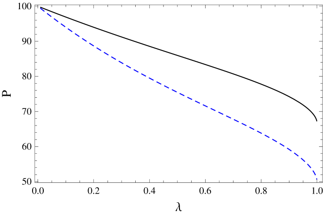
Figure 4: These curves show the behavior of ${\rm P}\left(\lambda\right)$ considering the whole diagram (continuous line) and only the region defined by the flat slicing (dashed line). In both cases ${\rm P}\left(\lambda\right)$ decreases for increasing values of $\lambda$. Nevertheless, its minimum is above $50$, which means that even in the worst case the foliation would cover most of the outside space.

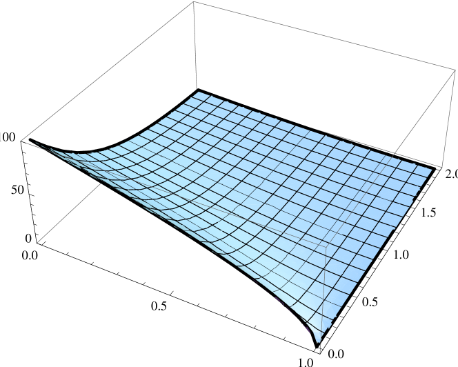
Figure 5: Portion of the future light cone of the bubble center covered by the CMC foliation in the inside space. We have only shown values of $\beta$ in the interval $[0,\,2]$.

Up to now we have pointed out that the use of foliation I could lead to satisfactory results regarding our typicality. However, we must also consider whether we are taking a suitably approximation when considering this foliation. Therefore, we should study the portion of the C-P diagram which is covered by the foliation. In the first place, we consider the whole outside space. We can roughly estimate the area being covered by the foliation in the diagram by approximating the area covered by the curves by the area covered by the lines which have the same endpoints. In the second place, we consider only the region of the diagram defined by the flat slicing, assuming $\Omega=1$. In Fig. 4 we show the behavior of ${\rm P}\left(\lambda\right)=100\times{\rm A}_{\rm cov}/{\rm A}_{\rm tot}$ in both cases. The foliation covers most of the outside space (${\rm P}\left(\lambda\right)>50\%$) independently of the particular decay model, considering both $\Omega>1$ and $\Omega=1$. On the other hand, following a similar procedure as that applied in the outside space, one can obtain the portion of the future light cone of the bubble center covered by the foliation, ${\rm P}_{b}\left(\lambda_{b},\,\beta\right)$, see Fig. 5. It can be noticed that the foliation is able to cover most part of the inside space only for very particular TVB decay models. However, that portion takes larger values considering the whole inside region, and the total portion, considering both regions, takes values even larger. Therefore, in the cases that this total portion is larger than $50\%$, one can suitably approximate the events of this spacetime by using this CMC foliation, and, at the end of the day, one could even conclude that we are typical observers by taking a suitable measure when defining probabilities. In the other cases, it should be worth noticed that to define probabilities for the occurrence of the events in this spacetime, one must not only add up the events of each hypersurface taking a certain measure, but also count the contribution of each region of the whole space; therefore, the use of this foliation could also provide us with an accurate approximation in those cases, if our region contributes more to the path integral, as it has been already suggested Page:2008zh .

- (1) S. R. Coleman and F. De Luccia, Phys. Rev. D 21 (1980) 3305.
- (2) S. R. Coleman, Phys. Rev. D 15 (1977) 2929 [Erratum-ibid. D 16 (1977) 1248].
- (3) A. D. Linde, Mod. Phys. Lett. A 1, (1986) 81.
- (4) J. Garriga and A. Vilenkin, Phys. Rev. D 57, (1998) 2230 [arXiv:astro-ph/9707292].
- (5) D. Yamauchi, A. Linde, A. Naruko, M. Sasaki and T. Tanaka, arXiv:1105.2674 [hep-th].
- (6) L. Susskind,“The anthropic landscape of string theory”, in Universe or multiverse?, B. Carr, ed. Cambridge Univ. Press, 2007. arXiv:hep-th/0302219.
- (7) D. N. Page, JCAP 0810, (2008) 025. [arXiv:0808.0351 [hep-th]].
- (8) J. W. York, Phys. Rev. Lett. 28 (1972), 1082-1085.
- (9) K. Kuchar, J. Math. Phys. 13 (1972) 768.
- (10) J. Barbour and N. O. Murchadha, arXiv:1009.3559 [gr-qc].
- (11) J. Metzger, Class. Quant. Grav. 21 (2004) 4625 [arXiv:gr-qc/0408059].
- (12) W. Israel, Nuovo Cim. B 44S10 (1966) 1 [Erratum-ibid. B 48 (1967 NUCIA,B44,1.1966) 463].
- (13) S. W. Hawking and G. F. R. Ellis, The Large Scale Structure of Space-Time, Cambridge University Press 1973.
- (14) K. M. Lee and E. J. Weinberg, Phys. Rev. D 36 (1987) 1088.
- (15) J. R. Gott, Nature 295 (1982) 304.
- (16) M. Bucher, A. S. Goldhaber and N. Turok, Phys. Rev. D 52 (1995) 3314 [arXiv:hep-ph/9411206].
- (17) V. A. Berezin, V. A. Kuzmin and I. I. Tkachev, Phys. Lett. B 120 (1983) 91.
- (18) S. J. Parke, Phys. Lett. B 121 (1983) 313.
- (19) E. Farhi and A. H. Guth, Phys. Lett. B 183 (1987) 149.
- (20) S. Ansoldi and E. I. Guendelman, Prog. Theor. Phys. 120 (2008) 985 [arXiv:0706.1233 [gr-qc]].
- (21) B. H. Lee, C. H. Lee, W. Lee, S. Nam and C. Park, Phys. Rev. D 77 (2008) 063502 [arXiv:0710.4599 [hep-th]].
- (22) J. E. Marsden and F. J. Tipler, Phys. Rep. 66 109-139 (1980).
- (23) R. Beig and J. M. Heinzle, Commun. Math. Phys. 260, 673-709 (2005) [gr-qc/0501020]; J. M. Heinzle, Phys. Rev. D 83 (2011) 084004 [arXiv:1105.1987 [gr-qc]].
- (24) E. Malec and N. O. Murchadha, Phys. Rev. D 80 (2009) 024017 [arXiv:0903.4779 [gr-qc]]; K. Sakai and Y. Satoh, JHEP 1003 (2010) 077 [arXiv:1001.1553 [hep-th]];
- (25) P. de Bernardis et al. [Boomerang Collaboration], Nature 404 (2000) 955 [arXiv:astro-ph/0004404].