KUNS-2329

Relativistic viscoelastic fluid mechanics

Masafumi Fukuma  and  Yuho Sakatani

Department of Physics, Kyoto University
Kyoto 606-8502, Japan

A detailed study is carried out for the relativistic theory of viscoelasticity which was recently constructed on the basis of Onsager’s linear nonequilibrium thermodynamics. After rederiving the theory using a local argument with the entropy current, we show that this theory universally reduces to the standard relativistic Navier-Stokes fluid mechanics in the long time limit. Since effects of elasticity are taken into account, the dynamics at short time scales is modified from that given by the Navier-Stokes equations, so that acausal problems intrinsic to relativistic Navier-Stokes fluids are significantly remedied. We in particular show that the wave equations for the propagation of disturbance around a hydrostatic equilibrium in Minkowski spacetime become symmetric hyperbolic for some range of parameters, so that the model is free of acausality problems. This observation suggests that the relativistic viscoelastic model with such parameters can be regarded as a causal completion of relativistic Navier-Stokes fluid mechanics. By adjusting parameters to various values, this theory can treat a wide variety of materials including elastic materials, Maxwell materials, Kelvin-Voigt materials, and (a nonlinearly generalized version of) simplified Israel-Stewart fluids, and thus we expect the theory to be the most universal description of single-component relativistic continuum materials. We also show that the presence of strains and the corresponding change in temperature are naturally unified through the Tolman law in a generally covariant description of continuum mechanics.

1 Introduction

The dynamics of fluids at large scales is universally described by the Navier-Stokes equations, which represent the regression to a global equilibrium with transfers of conserved quantities (such as energy-momentum and particle number) among fluid particles [1]. This can be formulated in a generally covariant way, but it is known that there arises a problem of acausality. In fact, the obtained equations for the propagation of disturbance are basically parabolic and thus predict infinitely large speed of propagation for infinitely high frequency modes, leaving light cones. One should note here that this does not imply the breakdown of the internal consistency of the description because the Navier-Stokes equations are simply an effective description at large spacetime scales and need not describe high frequency modes correctly. However, this is still troublesome when adopting the equations in numerical simulations; the initial value problems are ill posed, and unacceptable numerical solutions can be obtained easily.

To remedy the problem, Müller, Israel, and Stewart [2, 3, 4] extended the theory by treating the dissipative part of stress tensor, $\tau^{\mu\nu}_{\rm(d)}$ , and the heat flux $q^{\mu}$ (for the Eckart frame) or the particle diffusion current $\nu^{\mu}$ (for the Landau-Lifshitz frame) as additional thermodynamic variables on which the entropy density can depend. This prescription is based on the so-called extended thermodynamics and corresponds to taking into account higher derivative corrections to the effective theory. It has been shown that such modified theories have a good causal behavior and that linear perturbations around a hydrostatic equilibrium obey hyperbolic differential equations. This is now regarded as a fundamental framework for the numerical study of relativistic viscous fluids.

Meanwhile, modifications of the Navier-Stokes equations have also been studied in the area of rheology, and the materials treated there are generically called viscoelastic materials or viscoelastic fluids. Historically, viscoelasticity was defined by Maxwell in the 19th century as the characteristic property of such continuum materials that behave as elastic solids at short time scales and as viscous fluids at long time scales [1, 5]. In 1948, Eckart proposed a theory of elasticity and anelasticity [6], which describes the nonrelativistic dynamics of single-component viscoelastic materials and was reinvented recently [7] in the light of the covariance under foliation preserving diffeomorphisms. In this description, elastic strains (or equivalently, the “intrinsic metric” defined below) are introduced as additional thermodynamic variables, as in the theory of elasticity. As explicitly shown in [7], this theory of viscoelasticity contains the theory of elasticity and the theory of fluids as special limiting cases, and correctly reproduces the Navier-Stokes equations in the fluid limit. Furthermore, as was pointed out in [8], since the dynamics at short time scales is dominated by elasticity, shear modes of linear perturbations around a hydrostatic equilibrium obey differential equations with second-order time derivatives (in contrast to the equations obtained from the Navier-Stokes equations that contain only a first-order time derivative), so that causal behaviors for large frequencies are significantly improved.

Recently, on the basis of Onsager’s linear regression theory on nonequilibrium thermodynamics [9, 10, 11, 12], the present authors proposed a relativistic theory of viscoelasticity [13] which generalizes the theory of elasticity and anelasticity [6, 7] in a generally covariant form. In the present paper, after rederiving the theory relying on a local argument with the entropy current, we study the detailed properties of relativistic viscoelasticity. We show that fluidity is universally realized in the long time limit and also that acausal problems disappear for a wide region of parameters. Thus, the relativistic theory of viscoelasticity with such parameters can be regarded as a causal completion of relativistic Navier-Stokes fluid mechanics, and we expect that it could be used as another basis in the numerical study of relativistic viscous fluids.

This paper is organized as follows. In Sec. 2 we rederive the viscoelastic model of [13] using a local argument with the entropy current. We also show that the presence of strains and the corresponding change in temperature are naturally unified in a generally covariant description of continuum mechanics. In Sec. 3 we consider the long and short time limits of our viscoelastic model. We prove that the model universally gives relativistic Navier-Stokes fluids in the long time limit. In Sec. 4 we show that when some parameters take specific values, our viscoelastic model reduces to (a higher-dimensional extension of) the nonlinear generalization of the simplified Israel-Stewart model [14]. In Sec. 5 we consider linear perturbations around a hydrostatic equilibrium in Minkowski spacetime. The dispersion relations show that the evolutions are certainly stable. Although the wave equations for the linear perturbations are not always hyperbolic, if some parameters are chosen appropriately (including the parametrizations for the simplified Israel-Stewart model) they become symmetric hyperbolic and thus free of acausality problems. Section 6 is devoted to conclusion and discussions.

2 Relativistic viscoelastic mechanics

In this section, we rederive the fundamental equations for relativistic viscoelastic mechanics using a local argument with the entropy current. In Appendix A we show that the present formulation is equivalent to the “entropic formulation” proposed in our previous paper [13] which is based on Onsager’s linear regression theory.

2.1 Definitions

We start by giving a brief review on the generally covariant definitions of viscoelastic materials [13].

Geometrical setup

We consider a single-component continuum material living in a $(D+1)$-dimensional Lorentzian manifold $\mathcal{M}$ . The local coordinates are denoted by $x^{\mu}$ $(\mu=0,1,\cdots,D)$ , and the background Lorentzian metric with signature $(-,+,\cdots,+)$ by $g_{\mu\nu}(x)$ . Following the convention of Landau and Lifshitz [1], we define the velocity field $u=u^{\mu}(x)\partial_{\mu}$ from the momentum $(D+1)$-vector $p_{\mu}$ as

$$u^{\mu}(x)\equiv g^{\mu\nu}(x)\,p_{\nu}(x)/e(x)=p^{\mu}(x)/e(x)\,,$$ (2.1)

where $e(x)\equiv\sqrt{-g^{\mu\nu}(x)\,p_{\mu}(x)\,p_{\nu}(x)}$ is the proper energy density. Note that $u^{\mu}(x)$ is normalized as $g_{\mu\nu}(x)u^{\mu}(x)u^{\nu}(x)=-1$ . Here and hereafter indices are subscripted (or superscripted) always with $g_{\mu\nu}$ (or with its inverse $g^{\mu\nu}$).

Assuming that the velocity field is hypersurface orthogonal, we introduce a foliation of $\mathcal{M}$ consisting of spatial hypersurfaces (timeslices) orthogonal to $u^{\mu}$ . We parametrize the timeslices with a real parameter $t$ and denote them by $\Sigma_{t}$ . We exclusively (except for Sec. 5) use a coordinate system $x=(x^{\mu})=(x^{0},\,{\boldsymbol{x}})$ such that $x^{0}=t$ , ${\boldsymbol{x}}=(x^{i})$ $(i=1\,,\cdots,D)$ , for which the shape of the material at time $t$ is given by the induced metric on $\Sigma_{t}$ :

$$h_{\mu\nu}(x)\equiv g_{\mu\nu}(x)+u_{\mu}(x)\,u_{\nu}(x)=g_{\mu\nu}(x)+\frac{p_{\mu}(x)\,p_{\nu}(x)}{e^{2}(x)}\,.$$ (2.2)

We also define the extrinsic curvature $K_{\mu\nu}$ of the hypersurface as half the Lie derivative of $h_{\mu\nu}$ with respect to the velocity field $u=u^{\mu}\partial_{\mu}$ :

$$K_{\mu\nu}\equiv\frac{1}{2}\,\pounds_{u}h_{\mu\nu}=\frac{1}{2}\,h_{\mu}^{~{}\rho}h_{\nu}^{~{}\sigma}\bigl{(}\nabla_{\rho}u_{\sigma}+\nabla_{\sigma}u_{\rho}\bigr{)}\,.$$ (2.3)

This measures the rate of change in the induced metric $h_{\mu\nu}$ as material particles flow along $u^{\mu}$. Note that this tensor is symmetric and orthogonal to $u^{\mu}$, $K_{\mu\nu}\,u^{\nu}=0$ .

In the ADM parametrization, the metric and the velocity are represented with the lapse $N(x)$ and the shifts $N^{i}(x)$ $(i=1,\cdots,D)$ as

$${\mathrm{d}}s^{2} =g_{\mu\nu}(x)\,{\mathrm{d}}x^{\mu}\,{\mathrm{d}}x^{\nu}=-N^{2}(x)\,{\mathrm{d}}t^{2}+h_{ij}(x)\,\bigl{(}{\mathrm{d}}x^{i}-N^{i}(x)\,{\mathrm{d}}t\bigr{)}\,\bigl{(}{\mathrm{d}}x^{j}-N^{j}(x)\,{\mathrm{d}}t\bigr{)}\,,$$ (2.4)

$$u =u^{\mu}(x)\,\partial_{\mu}=\frac{1}{N(x)}\,\partial_{0}+\frac{N^{i}(x)}{N(x)}\,\partial_{i}\quad\bigl{(}\Leftrightarrow~{}u_{\mu}(x)\,{\mathrm{d}}x^{\mu}=-N(x)\,{\mathrm{d}}t\bigr{)}\,.$$ (2.5)

The volume element on the hypersurface is given by the $D$-form $\sqrt{h}\,{\mathrm{d}}^{D}{\boldsymbol{x}}\equiv\sqrt{\det(h_{ij})}\,{\mathrm{d}}^{D}{\boldsymbol{x}}=N^{-1}\sqrt{-g}\,{\mathrm{d}}^{D}{\boldsymbol{x}}$ .

With a given foliation, we still have the symmetry of foliation preserving diffeomorphisms that give rise to transformations only among the points on each timeslice. Using this residual gauge symmetry we can impose the synchronized gauge, $N^{i}(x)\equiv 0$ , so that the background metric and the velocity field are expressed as

$${\mathrm{d}}s^{2} =g_{\mu\nu}(x)\,{\mathrm{d}}x^{\mu}\,{\mathrm{d}}x^{\nu}\equiv-N^{2}(x)\,{\mathrm{d}}t^{2}+h_{ij}(x)\,{\mathrm{d}}x^{i}\,{\mathrm{d}}x^{j}\,,$$ (2.6)

$$u =u^{\mu}(x)\,\partial_{\mu}=\frac{1}{N(x)}\,\frac{\partial}{\partial t}=\frac{\partial}{\partial\tau}\,,$$ (2.7)

where $\tau$ is the local proper time defined by ${\mathrm{d}}\tau=N\,{\mathrm{d}}t$ . In this gauge, due to the relation $\partial/\partial t=N(x)\,\partial/\partial\tau$ , the proper energy density $e(x)$ measured with the proper time $\tau$ is related to the energy density ${\mathsf{e}}(x)$ measured with time $t$ as

$${\mathsf{e}}(x)=N(x)\,e(x)\,.$$ (2.8)

Note that ${\mathsf{e}}(x)$ includes the gravitational potential through the factor $N(x)$ . Accordingly, the local temperature $T$ measured with $\tau$ is related to the temperature ${\mathsf{T}}$ measured with $t$ through the following Tolman law:

$${\mathsf{T}}(x)=N(x)\,T(x)\,.$$ (2.9)

Definition of (relativistic) viscoelastic materials

According to the definition of Maxwell, viscoelastic materials behave as elastic solids at short time scales and as viscous fluids at long time scales (see, e.g., Sec. 36 in [5]). In order to understand how such materials evolve in time, we consider a material consisting of many molecules bonding each other and assume that the molecules first stay at their equilibrium positions in the absence of strains (as in the leftmost illustration of Fig. 1) [7, 8].

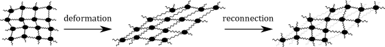
Figure 1: Processes of deformation and stress relaxation [7, 8].

We now suppose that an external force is applied to deform the material. An internal strain is then produced in the body, and according to the definition, the accompanied internal stress can be treated as an elastic force at least during short intervals of time. However, if we keep the deformation much longer than the relaxation times (characteristic to each material), then the bonding structure changes to maximize the entropy, and the internal strain vanishes eventually as in the rightmost of Fig. 1. The point is that two figures (the central and the rightmost) have the same shape (same induced metric) $h_{\mu\nu}$ , but different bonding structures.

The internal bonding structure can be specified by the intrinsic metric $\bar{h}_{\mu\nu}$ , which measures the shape that the material would take when all the internal strains are removed virtually [6, 7]. For the example given in Fig. 1, the intrinsic metric for the center illustration is given by the induced metric for the leftmost illustration, while the intrinsic metric for the rightmost illustration agrees with the induced metric for itself. Thus, the plastic (i.e., nonelastic) deformation from the center illustration to the rightmost illustration is described as the evolution of the intrinsic metric.

Its generally covariant generalization can be defined in the following way. Suppose that we have two adjacent, spatially separated spacetime points $P$ and $Q$ , each of which represents a point on the trajectory of a material particle (see Fig. 2).

Figure 2: Real ($x^{\mu}(\tau)$) and virtual ($\bar{x}^{\mu}(\tau)$) trajectories of material particles. The distance between $\bar{P}$ and $\bar{Q}$ gives the definition of the intrinsic metric $\bar{g}_{\mu\nu}$ .

By denoting their coordinates by $x=(x^{\mu})$ and $x+{\mathrm{d}}x=(x^{\mu}+{\mathrm{d}}x^{\mu})$ , respectively, the distance between $P$ and $Q$ in the real configuration is of course given with the metric $g_{\mu\nu}$ as (the square root of)

$${\mathrm{d}}s^{2}=g_{\mu\nu}(x)\,{\mathrm{d}}x^{\mu}\,{\mathrm{d}}x^{\nu}\,.$$ (2.10)

We now virtually remove all the strains in a sufficiently small spacetime region including the two points. Then $P$ and $Q$ would move to other positions $\bar{P}$ and $\bar{Q}$, whose coordinates we denote by $\bar{x}=(\bar{x}^{\mu})$ and $\bar{x}+{\mathrm{d}}\bar{x}=(\bar{x}^{\mu}+{\mathrm{d}}\bar{x}^{\mu})$ , respectively. This correspondence defines a local map $f:\,x\mapsto\bar{x}=\bar{x}(x)$ , with which we define the intrinsic metric $\bar{g}_{\mu\nu}(x)$ as the metric measuring the virtual distance between $\bar{P}$ and $\bar{Q}$ (or, as the pullback of the metric $g_{\mu\nu}$ for the map; $\bar{g}_{\mu\nu}\equiv f^{\ast}g_{\mu\nu}$):

$${\mathrm{d}}\bar{s}^{2} \equiv g_{\rho\sigma}(\bar{x})\,{\mathrm{d}}\bar{x}^{\rho}\,{\mathrm{d}}\bar{x}^{\sigma}=g_{\rho\sigma}\bigl{(}\bar{x}(x)\bigr{)}\,\frac{\partial\bar{x}^{\rho}}{\partial x^{\mu}}\,\frac{\partial\bar{x}^{\sigma}}{\partial x^{\nu}}\,{\mathrm{d}}x^{\mu}\,{\mathrm{d}}x^{\nu}$$

$$\equiv\bar{g}_{\mu\nu}(x)\,{\mathrm{d}}x^{\mu}\,{\mathrm{d}}x^{\nu}\,.$$ (2.11)

With the velocity vector $u=u^{\mu}(x)\,\partial_{\mu}$ , we parametrize $\bar{g}_{\mu\nu}$ as

$$\bar{g}_{\mu\nu} =-(1+2\theta)\,u_{\mu}u_{\nu}-\varepsilon_{\mu}u_{\nu}-\varepsilon_{\nu}\,u_{\mu}+\bar{h}_{\mu\nu}$$

$$\bigl{(}\varepsilon_{\mu}u^{\mu}=0\,,\quad h_{\mu\nu}\,u^{\nu}=0\,,\quad\bar{h}_{\mu\nu}\,u^{\nu}=0\bigr{)}\,.$$ (2.12)

The strain tensor is then introduced as

$$E_{\mu\nu}(x) \equiv\frac{1}{2}\,\bigl{(}g_{\mu\nu}(x)-\bar{g}_{\mu\nu}(x)\bigr{)}$$

$$=\,\theta\,u_{\mu}u_{\nu}+\frac{1}{2}\,\bigl{(}\varepsilon_{\mu}u_{\nu}+\varepsilon_{\nu}\,u_{\mu}\bigr{)}+\varepsilon_{\mu\nu}\,,$$ (2.13)

where

$$\varepsilon_{\mu\nu}(x)\equiv\frac{1}{2}\,\bigl{(}h_{\mu\nu}(x)-\bar{h}_{\mu\nu}(x)\bigr{)}$$ (2.14)

is the spatial strain tensor. Note that if we define the extrinsic curvature associated with the spatial intrinsic metric $\bar{h}_{\mu\nu}$ as

$$\bar{K}_{\mu\nu}\equiv\frac{1}{2}\,\pounds_{u}\bar{h}_{\mu\nu}=\frac{1}{2}\,\bigl{(}u^{\lambda}\,\partial_{\lambda}\bar{h}_{\mu\nu}+\partial_{\mu}u^{\lambda}\,\bar{h}_{\lambda\nu}+\partial_{\nu}u^{\lambda}\,\bar{h}_{\mu\lambda}\bigr{)}\,,$$ (2.15)

the following identity holds:

$$\pounds_{u}\varepsilon_{\mu\nu}=K_{\mu\nu}-\bar{K}_{\mu\nu}\,.$$ (2.16)

A viscoelastic material is a thermodynamic system consisting of material particles as its subsystems. While the system regresses to a thermodynamic equilibrium, one can imagine that the virtual trajectory of each material particle approaches its real trajectory, so that the strain tensor $E_{\mu\nu}$ approaches zero. Such an irreversible process is called plastic (i.e., nonelastic), and thus we see that the dynamics of $E_{\mu\nu}$ includes plastic evolutions (in addition to reversible, elastic evolutions). In the following discussions, we assume that $E_{\mu\nu}=(\varepsilon_{\mu\nu}\,,\,\varepsilon_{\mu}\,,\,\theta)$ are all small quantities, such that their nonlinear effects can be neglected. We shall denote the contraction of a spatial tensor $A_{\mu\nu}$ with $g^{\mu\nu}$ by $\operatorname{tr}A$ , so that

$$\operatorname{tr}\varepsilon\equiv g^{\mu\nu}\varepsilon_{\mu\nu}=h^{\mu\nu}\varepsilon_{\mu\nu}\,,\quad\operatorname{tr}K\equiv g^{\mu\nu}K_{\mu\nu}=h^{\mu\nu}K_{\mu\nu}\,.$$ (2.17)

We close this section by explaining the physical meaning of the strain tensor $E_{\mu\nu}=(\varepsilon_{\mu\nu}\,,\,\varepsilon_{\mu}\,,\,\theta)$ . The spatial strain tensor $\varepsilon_{\mu\nu}$ stands for the standard strains, measuring the difference between the induced metric $h_{\mu\nu}$ and the spatial induced metric $\bar{h}_{\mu\nu}$ . One can easily see that the quantity $\varepsilon^{\mu}$ represents the relative velocity of a material particle in its real trajectory with respect to that in its virtual trajectory, $\varepsilon^{\mu}=u^{\mu}-\bar{u}^{\mu}\equiv{\mathrm{d}}x^{\mu}/{\mathrm{d}}\tau-{\mathrm{d}}\bar{x}^{\mu}/{\mathrm{d}}\tau$ , where $\tau$ is a common proper time (see Fig. 2). In order to understand the meaning of $\theta$, we first recall that the covariant vector $u_{\mu}$ is expressed as $u_{\mu}\,{\mathrm{d}}x^{\mu}=-N\,{\mathrm{d}}x^{0}$ . We can then rewrite ${\mathrm{d}}s^{2}$ and ${\mathrm{d}}\bar{s}^{2}$ as

$${\mathrm{d}}s^{2} =-\,N^{2}(x)\,({\mathrm{d}}x^{0})^{2}+h_{\mu\nu}(x)\,{\mathrm{d}}x^{\mu}\,{\mathrm{d}}x^{\nu}\,,$$ (2.18)

$${\mathrm{d}}\bar{s}^{2} =-\,\bigl{(}1+2\theta(x)\bigr{)}\,N^{2}(x)\,({\mathrm{d}}x^{0})^{2}+2N(x)\,\varepsilon_{\mu}(x)\,{\mathrm{d}}x^{\mu}\,{\mathrm{d}}x^{0}+\bar{h}_{\mu\nu}(x)\,{\mathrm{d}}x^{\mu}\,{\mathrm{d}}x^{\nu}\,,$$ (2.19)

with $h_{\mu\nu}\,{\mathrm{d}}x^{\mu}\,{\mathrm{d}}x^{\nu}=h_{ij}\,({\mathrm{d}}x^{i}-N^{i}\,{\mathrm{d}}x^{0})\,({\mathrm{d}}x^{j}-N^{j}\,{\mathrm{d}}x^{0})$ and a similar (but a bit more complicated) expression for $2N\,\varepsilon_{\mu}\,{\mathrm{d}}x^{\mu}\,{\mathrm{d}}x^{0}+\bar{h}_{\mu\nu}\,{\mathrm{d}}x^{\mu}\,{\mathrm{d}}x^{\nu}$ . These equations mean that $\bar{N}\equiv\sqrt{1+2\theta}\,N\simeq(1+\theta)\,N$ represents the lapse function for the intrinsic metric. Then, through the Tolman law, we can relate the virtual temperature $\bar{T}$ observed in the absence of strains to the actual temperature $T$ as $N\,T=\bar{N}\,\bar{T}\,(={\mathsf{T}})$ . We thus obtain the relation $\theta=(\bar{N}^{2}/N^{2}-1)/2=(T^{2}/\bar{T}^{2}-1)/2\simeq(T-\bar{T})/\bar{T}$, and conclude that the scalar $\theta$ expresses the increase of the temperature due to strains. This conclusion shows that the presence of strains and the corresponding change in temperature are naturally unified in a generally covariant description of continuum mechanics.

2.2 Entropy production rate

As was adopted in [13], in order to develop thermodynamics in a generally covariant manner, it is convenient to distinguish density quantities from other intensive quantities, and, by multiplying them with the spatial volume element $\sqrt{h}$ , we construct new quantities which are spatial densities on each timeslice. For example, the entropy density $s$, the energy-momentum density $p_{\mu}$ , and the number density $n$ are density quantities, and for them we introduce the following spatial densities:

$${\tilde{s}}\equiv\sqrt{h}\,s\,,\quad{\tilde{p}}_{\mu}\equiv\sqrt{h}\,p_{\mu}\,,\quad{\tilde{n}}\equiv\sqrt{h}\,n\,.$$ (2.20)

We assume that each material particle is in its local thermodynamic equilibrium, and that the local entropy ${\tilde{s}}$ is a function of ${\tilde{p}}_{\mu}$ , ${\tilde{n}}$ , and $g_{\mu\nu}$ as well as of the strain tensor $E_{\mu\nu}=(\varepsilon_{\mu\nu}\,,\,\varepsilon_{\mu}\,,\,\theta)$ :

$${\tilde{s}}(x)={\tilde{s}}\bigl{(}E_{\mu\nu}(x),{\tilde{p}}_{\mu}(x),{\tilde{n}}(x),g_{\mu\nu}(x)\bigr{)}\,.$$ (2.21)

We further assume that ${\tilde{s}}$ depends on ${\tilde{p}}_{\mu}$ only through the local proper energy ${\tilde{e}}({\tilde{p}}_{\mu},\,g_{\mu\nu})\equiv\sqrt{-g^{\mu\nu}\,{\tilde{p}}_{\mu}\,{\tilde{p}}_{\nu}}$ , so that ${\tilde{s}}$ can also be expressed as

$${\tilde{s}}(x) ={\tilde{\sigma}}\bigl{(}E_{\mu\nu}(x)\,,\,{\tilde{e}}(x)\,,\,{\tilde{n}}(x)\,,\,g_{\mu\nu}(x)\bigr{)}$$

$$={\tilde{\sigma}}\bigl{(}\varepsilon_{\mu\nu}(x)\,,\,\varepsilon_{\mu}(x)\,,\,\theta(x)\,,\,{\tilde{e}}({\tilde{p}}_{\mu}(x),g_{\mu\nu}(x))\,,{\tilde{n}}(x)\,,\,g_{\mu\nu}(x)\bigr{)}\,.$$ (2.22)

Since we are only interested in linear nonequilibrium thermodynamics, we only need to expand ${\tilde{s}}$ in $E_{\mu\nu}$ to second order:

$${\tilde{s}} =\mbox{(terms independent of $E_{\mu\nu}$)}$$

$$~{}~{}~{}~{}-\frac{1}{2T}\bigl{[}2\lambda_{1}\varepsilon_{\langle\mu\nu\rangle}\varepsilon^{\langle\mu\nu\rangle}+\lambda_{2}\,\varepsilon_{\mu}\varepsilon^{\mu}+\gamma_{1}\,(\operatorname{tr}\varepsilon)^{2}+2\gamma_{2}\,(\operatorname{tr}\varepsilon)\,\theta+\gamma_{3}\,\theta^{2}\bigr{]}\,.$$ (2.23)

We require the stability of the system under the change in strains $E_{\mu\nu}$ , so that the constants $\lambda_{1}$ and $\lambda_{2}$ are non-negative, and the matrix ${\boldsymbol{\gamma}}=\bigl{(}\begin{smallmatrix}\gamma_{1}&\gamma_{2}\cr\gamma_{2}&\gamma_{3}\end{smallmatrix}\bigr{)}$ is positive semidefinite.

Then the fundamental thermodynamic relation can be written as

$$\delta{\tilde{s}}= ~{}-\frac{u^{\nu}}{T}\,\delta{\tilde{p}}_{\nu}-\frac{\mu}{T}\,\delta{\tilde{n}}+\frac{\sqrt{h}}{2T}\,T^{\mu\nu}_{\mathrm{(q)}}\,\delta g_{\mu\nu}$$

$$~{}-\frac{\sqrt{h}}{T}\,2\lambda_{1}\,\varepsilon^{\langle\mu\nu\rangle}\,\delta\varepsilon_{\langle\mu\nu\rangle}-\frac{\sqrt{h}}{T}\,\bigl{(}\gamma_{1}\,\operatorname{tr}\varepsilon+\gamma_{2}\,\theta\bigr{)}\,\delta(\operatorname{tr}\varepsilon)$$

$$~{}-\frac{\sqrt{h}}{T}\,\lambda_{2}\,\varepsilon^{\mu}\,\delta\varepsilon_{\mu}-\frac{\sqrt{h}}{T}\,\bigl{(}\gamma_{3}\,\theta+\gamma_{2}\,\operatorname{tr}\varepsilon\bigr{)}\,\delta\theta\,.$$ (2.24)

Here the temperature $T$ , the chemical potential $\mu$ and the quasiconservative part of the stress tensor, $\tau_{\mathrm{(q)}}^{\mu\nu}$ , are defined as

$$\frac{\partial{\tilde{\sigma}}}{\partial{\tilde{e}}}=\frac{1}{T}\,,\quad\frac{\partial{\tilde{\sigma}}}{\partial{\tilde{n}}}=-\frac{\mu}{T}\,,\quad\frac{\partial{\tilde{\sigma}}}{\partial g_{\mu\nu}}=\frac{\sqrt{h}}{2T}\,\tau_{\mathrm{(q)}}^{\mu\nu}\,,$$ (2.25)

where we require that $\tau^{\mu\nu}_{\mathrm{(q)}}$ be orthogonal to $u^{\mu}$ , $\tau^{\mu\nu}_{\mathrm{(q)}}\,u_{\nu}=0$ . The quasiconservative part of the energy-momentum tensor is then defined as

$$T^{\mu\nu}_{\mathrm{(q)}} \equiv e\,u^{\mu}u^{\nu}+\tau^{\mu\nu}_{\mathrm{(q)}}\,.$$ (2.26)

In deriving Eq. (2.24), we have used the relations

$$\frac{\partial{\tilde{e}}({\tilde{p}}_{\mu},g_{\mu\nu})}{\partial{\tilde{p}}_{\nu}}=-u^{\nu}\,,\qquad\frac{\partial{\tilde{e}}({\tilde{p}}_{\mu},g_{\mu\nu})}{\partial g_{\mu\nu}}=\frac{{\tilde{e}}}{2}\,u^{\mu}u^{\nu}\,.$$ (2.27)

We now set the variation in Eq. (2.24) to be $\delta=\pounds_{u}$ . We then obtain

$$\sqrt{h}\,\nabla_{\mu}(s\,u^{\mu})=\sqrt{h}\,\Big{[} -\frac{u^{\nu}}{T}\,\nabla_{\mu}(p_{\nu}\,u^{\mu})-\frac{\mu}{T}\,\nabla_{\mu}(n\,u^{\mu})+\frac{1}{T}\,\tau^{\mu\nu}_{\mathrm{(q)}}\,K_{\mu\nu}$$

$$-\frac{2\lambda_{1}}{T}\,\varepsilon^{\langle\mu\nu\rangle}\,\pounds_{u}\varepsilon_{\langle\mu\nu\rangle}-\frac{1}{T}\bigl{(}\gamma_{1}\,\operatorname{tr}\varepsilon+\gamma_{2}\,\theta\bigr{)}\,\pounds_{u}(\operatorname{tr}\varepsilon)$$

$$-\frac{\lambda_{2}}{T}\,\varepsilon^{\mu}\,\pounds_{u}\varepsilon_{\mu}-\frac{1}{T}\bigl{(}\gamma_{3}\,\theta+\gamma_{2}\,\operatorname{tr}\varepsilon\bigr{)}\,\pounds_{u}\theta\Big{]}\,.$$ (2.28)

Here we have used the identities for Lie derivatives:

$$\pounds_{u}\,{\tilde{s}}=\sqrt{h}\,\nabla_{\mu}\bigl{(}s\,u^{\mu})\,,\quad\pounds_{u}\,{\tilde{p}}_{\nu}=\sqrt{h}\,\nabla_{\mu}\bigl{(}p_{\nu}\,u^{\mu}\bigr{)}\,,\quad\pounds_{u}\,{\tilde{n}}=\sqrt{h}\,\nabla_{\mu}\bigl{(}n\,u^{\mu})\,,$$ (2.29)

which can be shown by using the identities $\pounds_{u}\sqrt{h}=\sqrt{h}\,\nabla_{\mu}u^{\mu}$ and $p_{\mu}\nabla_{\nu}u^{\mu}=0$ . Note that $\operatorname{tr}\bigl{(}\pounds_{u}\varepsilon_{\mu\nu}\bigr{)}=h^{\mu\nu}\,\pounds_{u}\varepsilon_{\mu\nu}$ can be replaced by $\pounds_{u}(\operatorname{tr}\varepsilon)$ in our approximation because the difference $\pounds_{u}(\operatorname{tr}\varepsilon)-\operatorname{tr}\bigl{(}\pounds_{u}\varepsilon_{\mu\nu}\bigr{)}=(\pounds_{u}\bar{h}^{\mu\nu})\,\varepsilon_{\mu\nu}=-2K^{\mu\nu}\,\varepsilon_{\mu\nu}$ is of higher orders.

The full energy-momentum tensor $T^{\mu\nu}$ and the full number current $n^{\mu}$ are given by

$$T^{\mu\nu} \equiv e\,u^{\mu}u^{\nu}+\tau^{\mu\nu}\,,\qquad n^{\mu}\equiv n\,u^{\mu}+\nu^{\mu}\,,$$

$$\bigl{(}\tau^{\mu\nu}u_{\nu}=0=\nu^{\mu}u_{\mu}\bigr{)}$$ (2.30)

where $\tau^{\mu\nu}$ and $\nu^{\mu}$ are the stress tensor and the diffusion current, respectively. Then, by introducing the entropy current

$$s^{\mu}\equiv s\,u^{\mu}-\frac{\mu}{T}\,\nu^{\mu}\,,$$ (2.31)

and by using Eq. (2.28) together with the current conservation laws

$$\nabla_{\nu}T^{\mu\nu}=0\,,\qquad\nabla_{\mu}n^{\mu}=0\,,$$ (2.32)

the local entropy production rate can be evaluated as

$$\nabla_{\mu}s^{\mu}= ~{}-\frac{1}{T}\,\bigl{(}\tau^{\mu\nu}-\tau_{\rm(q)}^{\mu\nu}\bigr{)}\,K_{\mu\nu}\,+\nu^{\mu}\,\partial_{\mu}\Bigl{(}-\frac{\mu}{T}\Bigr{)}$$

$$~{}-\frac{2\lambda_{1}}{T}\,\varepsilon^{\langle\mu\nu\rangle}\,\pounds_{u}\varepsilon_{\mu\nu}-\frac{1}{T}\,\bigl{(}\gamma_{1}\,\operatorname{tr}\varepsilon+\gamma_{2}\,\theta\bigr{)}\,\pounds_{u}\operatorname{tr}\varepsilon$$

$$~{}-\frac{\lambda_{2}}{T}\,\varepsilon^{\mu}\,\pounds_{u}\varepsilon_{\mu}-\frac{1}{T}\bigl{(}\gamma_{3}\,\theta+\gamma_{2}\,\operatorname{tr}\varepsilon\bigr{)}\,\pounds_{u}\theta$$

$$= ~{}\begin{pmatrix}\varepsilon^{\langle\mu\nu\rangle}&(-1/T)\,K^{\langle\mu\nu\rangle}\end{pmatrix}\begin{pmatrix}(-2\lambda_{1}/T)\,\pounds_{u}\varepsilon_{\langle\mu\nu\rangle}\cr\tau_{\langle\mu\nu\rangle}-\tau^{\rm(q)}_{\langle\mu\nu\rangle}\end{pmatrix}$$

$$~{}+\begin{pmatrix}\varepsilon^{\mu}&\nabla^{\mu}(-\mu/T)\end{pmatrix}\begin{pmatrix}(-\lambda_{2}/T)\,\pounds_{u}\varepsilon_{\mu}\cr\nu_{\mu}\end{pmatrix}$$

$$~{}+\begin{pmatrix}\operatorname{tr}\varepsilon&\theta&(-1/T)\,\operatorname{tr}K\end{pmatrix}\begin{pmatrix}-(1/T)\,{\boldsymbol{\gamma}}\,\begin{pmatrix}\pounds_{u}(\operatorname{tr}\varepsilon)\cr\pounds_{u}\theta\end{pmatrix}\cr(1/D)\,\bigl{(}\operatorname{tr}\tau-\operatorname{tr}\tau_{\mathrm{(q)}}\bigr{)}\end{pmatrix}\,.$$ (2.33)

Thus, if we require that each term be separately positive definite, we obtain the following equations:

$$\begin{pmatrix}-(2\lambda_{1}/T)\,\pounds_{u}\varepsilon_{\langle\mu\nu\rangle}\cr\tau_{\langle\mu\nu\rangle}-\tau_{\langle\mu\nu\rangle}^{\mathrm{(q)}}\end{pmatrix} =2\,({\boldsymbol{\mathcal{G}}}+{\boldsymbol{\eta}})\begin{pmatrix}\varepsilon_{\langle\mu\nu\rangle}\cr(-1/T)\,K_{\langle\mu\nu\rangle}\end{pmatrix}\,,$$ (2.34)

$$\begin{pmatrix}-(\lambda_{2}/T)\,\pounds_{u}\varepsilon_{\mu}\cr\nu_{\mu}\end{pmatrix} =({\boldsymbol{\mathcal{H}}}+{\boldsymbol{\sigma}})\begin{pmatrix}\varepsilon_{\mu}\cr h_{\mu}^{~{}\nu}\partial_{\nu}(-\mu/T)\end{pmatrix}\,,$$ (2.35)

$$\begin{pmatrix}-(1/T)\,{\boldsymbol{\gamma}}\,\begin{pmatrix}\pounds_{u}(\operatorname{tr}\varepsilon)\cr\pounds_{u}\theta\end{pmatrix}\cr(1/D)\bigl{(}\operatorname{tr}\tau-\operatorname{tr}\tau_{\mathrm{(q)}}\bigr{)}\end{pmatrix} =({\boldsymbol{\mathcal{K}}}+{\boldsymbol{\zeta}})\begin{pmatrix}\operatorname{tr}\varepsilon\cr\theta\cr(-1/T)\,\operatorname{tr}K\end{pmatrix}\,.$$ (2.36)

Here ${\boldsymbol{\mathcal{G}}}$ , ${\boldsymbol{\mathcal{H}}}$ , and ${\boldsymbol{\mathcal{K}}}$ are antisymmetric matrices,

$${\boldsymbol{\mathcal{G}}}=\begin{pmatrix}0&\mathcal{G}\cr-\mathcal{G}&0\end{pmatrix}\,,\quad{\boldsymbol{\mathcal{H}}}=\begin{pmatrix}0&\mathcal{H}\cr-\mathcal{H}&0\cr\end{pmatrix}\,,\quad{\boldsymbol{\mathcal{K}}}=\begin{pmatrix}0&\mathcal{K}^{\prime}&\mathcal{K}\cr-\mathcal{K}^{\prime}&0&-\mathcal{K}a\cr-\mathcal{K}&\mathcal{K}a&0\end{pmatrix}\,,$$ (2.37)

and ${\boldsymbol{\eta}}$ , ${\boldsymbol{\sigma}}$ , and ${\boldsymbol{\zeta}}$ are positive semidefinite symmetric matrices,

$${\boldsymbol{\eta}}=\begin{pmatrix}\eta_{1}&\eta_{2}\cr\eta_{2}&\eta_{3}\end{pmatrix}\,,\quad{\boldsymbol{\sigma}}=\begin{pmatrix}\sigma_{1}&\sigma_{2}\cr\sigma_{2}&\sigma_{3}\cr\end{pmatrix}\,,\quad{\boldsymbol{\zeta}}=\begin{pmatrix}\zeta_{1}&\zeta_{2}&\zeta_{4}\cr\zeta_{2}&\zeta_{3}&\zeta_{5}\cr\zeta_{4}&\zeta_{5}&\zeta_{6}\end{pmatrix}\,.$$ (2.38)

Note that only the symmetric matrices contribute when substituted to the entropy production rate (2.33). This means that the matrices ${\boldsymbol{\eta}}$ , ${\boldsymbol{\sigma}}$ , and ${\boldsymbol{\zeta}}$ are associated with irreversible processes, while the matrices ${\boldsymbol{\mathcal{G}}}$ , ${\boldsymbol{\mathcal{H}}}$ , and ${\boldsymbol{\mathcal{K}}}$ are with reversible ones.

The relationship between the equations given above and the corresponding ones given in [13] is summarized in Appendix A.

2.3 Fundamental equations

Using Eqs. (2.34)–(2.38) at each point $x=(x^{0}=t,\,{\boldsymbol{x}})$ on timeslice $\Sigma_{t}$ , we can express (A) the currents $\tau^{\mu\nu}$ and $\nu^{\mu}$ and (B) the evolution of strains, $\pounds_{u}\varepsilon_{\langle\mu\nu\rangle}\,,\ \pounds_{u}\varepsilon_{\mu}\,,\ \pounds_{u}\operatorname{tr}\varepsilon$ , and $\pounds_{u}\theta$ , only in terms of local thermodynamic quantities on $\Sigma_{t}$ .

We thus conclude that the dynamics of relativistic viscoelastic materials is described by the following two sets of equations [13, 7]:

(A) current conservation laws:

$$\nabla_{\mu}T^{\mu\nu} =\nabla_{\mu}\bigl{(}e\,u^{\mu}u^{\nu}+\tau^{\mu\nu}\bigr{)}=0\,,$$ (2.39)

$$\nabla_{\mu}n^{\mu} =\nabla_{\mu}\bigl{(}n\,u^{\mu}+\nu^{\mu}\bigr{)}=0\,,$$ (2.40)

with the constitutive equations

$$\tau^{\mu\nu}= ~{}\tau^{\mu\nu}_{\mathrm{(q)}}-2\,(\mathcal{G}-\eta_{2})\,\varepsilon^{\langle\mu\nu\rangle}-\frac{2\eta_{3}}{T}\,K^{\langle\mu\nu\rangle}$$

$$~{}-\Bigl{[}(\mathcal{K}-\zeta_{4})\,\operatorname{tr}\varepsilon-(\mathcal{K}a+\zeta_{5})\,\theta+\frac{\zeta_{6}}{T}\,\operatorname{tr}K\Bigr{]}\,h^{\mu\nu}\,,$$ (2.41)

$$\nu^{\mu}= ~{}-(\mathcal{H}-\sigma_{2})\,\varepsilon^{\mu}+\sigma_{3}\,h^{\mu\nu}\partial_{\nu}\Bigl{(}-\frac{\mu}{T}\Bigr{)}\,.$$ (2.42)

(B) rheology equations:

$$\pounds_{u}\varepsilon_{\langle\mu\nu\rangle} =-\frac{\eta_{1}\,T}{\lambda_{1}}\,\varepsilon_{\langle\mu\nu\rangle}+\frac{\mathcal{G}+\eta_{2}}{\lambda_{1}}\,K_{\langle\mu\nu\rangle}\,,$$ (2.43)

$$\pounds_{u}\varepsilon_{\mu} =-\frac{\sigma_{1}\,T}{\lambda_{2}}\varepsilon_{\mu}-\frac{(\mathcal{H}+\sigma_{2})\,T}{\lambda_{2}}h_{\mu}^{~{}\nu}\partial_{\nu}\Bigl{(}-\frac{\mu}{T}\Bigr{)}\,,$$ (2.44)

$$\begin{pmatrix}\pounds_{u}(\operatorname{tr}\varepsilon)\cr\pounds_{u}\theta\end{pmatrix} =\begin{pmatrix}\gamma_{1}&\gamma_{2}\cr\gamma_{2}&\gamma_{3}\end{pmatrix}^{-1}\begin{pmatrix}-\zeta_{1}\,T\,\operatorname{tr}\varepsilon-(\mathcal{K}^{\prime}+\zeta_{2})\,T\,\theta+(\mathcal{K}+\zeta_{4})\,\operatorname{tr}K\cr(\mathcal{K}^{\prime}-\zeta_{2})\,T\,\operatorname{tr}\varepsilon-\zeta_{3}\,T\,\theta-(\mathcal{K}a-\zeta_{5})\,\operatorname{tr}K\end{pmatrix}$$

$$=\begin{pmatrix}-\frac{(\gamma_{3}\,\zeta_{1}+\gamma_{2}\,(\mathcal{K}^{\prime}-\zeta_{2}))\,T}{\det{\boldsymbol{\gamma}}}\,\operatorname{tr}\varepsilon+\frac{(\gamma_{2}\,\zeta_{3}-\gamma_{3}\,(\mathcal{K}^{\prime}+\zeta_{2}))\,T}{\det{\boldsymbol{\gamma}}}\,\theta+\frac{\gamma_{3}\,(\mathcal{K}+\zeta_{4})+\gamma_{2}\,(\mathcal{K}a-\zeta_{5})}{\det{\boldsymbol{\gamma}}}\,\operatorname{tr}K\cr\frac{(\gamma_{2}\,\zeta_{1}+\gamma_{1}(\mathcal{K}^{\prime}-\zeta_{2}))\,T}{\det{\boldsymbol{\gamma}}}\,\operatorname{tr}\varepsilon-\frac{(\gamma_{1}\zeta_{3}-\gamma_{2}\,(\mathcal{K}^{\prime}+\zeta_{2}))\,T}{\det{\boldsymbol{\gamma}}}\,\theta-\frac{\gamma_{2}\,(\mathcal{K}+\zeta_{4})+\gamma_{1}\,(\mathcal{K}a-\zeta_{5})}{\det{\boldsymbol{\gamma}}}\,\operatorname{tr}K\end{pmatrix}\,.$$ (2.45)

The former set of equations describes the dynamics of $D+2$ conserved quantities $(p_{\mu}=e\,u_{\mu},\,n)$ , while the latter that of $D(D+1)/2$ dynamical variables $E_{\mu\nu}=(\varepsilon_{\mu\nu},\varepsilon_{\mu},\theta)$ .

It is convenient to introduce the following parameters:

$$\tau_{\mathrm{s}} \equiv\frac{\lambda_{1}}{\eta_{1}\,T}\,,\qquad\tau_{\sigma}\equiv\frac{\lambda_{2}}{\sigma_{1}\,T}\,,$$ (2.46)

$$\tau_{\pm} \equiv\frac{2\det{\boldsymbol{\gamma}}}{T\,\bigl{(}P_{\zeta\gamma}\mp\sqrt{P_{\zeta\gamma}^{2}-4\det{\boldsymbol{\gamma}}\,(\det{\boldsymbol{\zeta}}_{\mathrm{s}}+\mathcal{K}^{\prime 2})}\bigr{)}}\,,$$ (2.47)

$$a_{\pm} \equiv\frac{-2\bigl{(}\zeta_{3}\,\gamma_{2}-(\mathcal{K}^{\prime}+\zeta_{2})\,\gamma_{3}\bigr{)}}{\zeta_{3}\,\gamma_{1}-\zeta_{1}\,\gamma_{3}-2\mathcal{K}^{\prime}\,\gamma_{2}\pm\sqrt{P_{\zeta\gamma}^{2}-4\det{\boldsymbol{\gamma}}\,(\det{\boldsymbol{\zeta}}_{\mathrm{s}}+\mathcal{K}^{\prime 2})}}\,,$$ (2.48)

where $P_{\zeta\gamma}\equiv\zeta_{3}\gamma_{1}+\zeta_{1}\gamma_{3}-2\zeta_{2}\gamma_{2}\geq 0$ , and ${\boldsymbol{\zeta}}_{\mathrm{s}}$ is the principal submatrix of ${\boldsymbol{\zeta}}$ defined by ${\boldsymbol{\zeta}}_{\mathrm{s}}\equiv\bigl{(}\begin{smallmatrix}\zeta_{1}&\zeta_{2}\cr\zeta_{2}&\zeta_{3}\end{smallmatrix}\bigr{)}$ . Since ${\boldsymbol{\zeta}}_{\mathrm{s}}$ is positive semidefinite, $\det{\boldsymbol{\zeta}}_{\mathrm{s}}$ is non-negative. Note that $\tau_{\mathrm{s}}$ , $\tau_{\sigma}$ , and $\mathrm{Re}\,\tau_{\pm}$ are all non-negative. We further introduce the scalar variables

$$\varepsilon_{\pm}\equiv\frac{1}{2}\,(\operatorname{tr}\varepsilon-a_{\pm}\,\theta)\,.$$ (2.49)

Then the rheology equations (2.43)–(2.45) can be rewritten in a more compact form:

(B${}^{\,\prime}$) rheology equations:

$$\pounds_{u}\varepsilon_{\langle\mu\nu\rangle}= ~{}-\frac{1}{\tau_{\mathrm{s}}}\,\varepsilon_{\langle\mu\nu\rangle}+\frac{\mathcal{G}+\eta_{2}}{\lambda_{1}}\,K_{\langle\mu\nu\rangle}\,,$$ (2.50)

$$\pounds_{u}\varepsilon_{\mu}= ~{}-\frac{1}{\tau_{\sigma}}\,\varepsilon_{\mu}-\frac{(\mathcal{H}+\sigma_{2})\,T}{\lambda_{2}}\,h_{\mu}^{~{}\nu}\,\partial_{\nu}\Bigl{(}-\frac{\mu}{T}\Bigr{)}\,,$$ (2.51)

$$\pounds_{u}\varepsilon_{\pm}= ~{}-\frac{1}{\tau_{\pm}}\,\varepsilon_{\pm}+\frac{(\mathcal{K}a-\zeta_{5})\,(a_{\pm}\,\gamma_{1}+\gamma_{2})+(\mathcal{K}+\zeta_{4})\,(a_{\pm}\,\gamma_{2}+\gamma_{3})}{2\det{\boldsymbol{\gamma}}}\,\operatorname{tr}K\,.$$ (2.52)

From these, we see that $\tau_{\mathrm{s}}$ , $\tau_{\sigma}$ , and $\mathrm{Re}\,\tau_{\pm}$ give the typical time scales for the relaxation of strains.

The relation between the viscoelastic models and a few well-known rheological models (such as the Maxwell model and the Kelvin-Voigt model) is discussed in Appendix B.

3 Fluid and elastic limits

In this section, we discuss the limits of elasticity and fluidity in the relativistic theory of viscoelasticity. We first identify the properties that characterize a given material as a fluid or as an elastic material. We then consider the long-time and short-time limits of our dynamical equations and show that fluidity is universally realized in the long time limit. We also make a comment on the subtlety existing in Maxwell’s definition of viscoelasticity.

3.1 Fluidity and elasticity

Fluidity is characterized by the property that the relaxation of the strains $E_{\mu\nu}=(\varepsilon_{\mu\nu},\,\varepsilon_{\mu},\,\theta)$ proceeds instantaneously. Thus, their rheology equations are expressed as

$$\pounds_{u}\varepsilon_{\mu\nu}=0\,,\quad\pounds_{u}\varepsilon_{\mu}=0\,,\quad\pounds_{u}\theta=0\,,\quad\mbox{(fluids)}$$ (3.1)

or equivalently,

$$\pounds_{u}\varepsilon_{\langle\mu\nu\rangle}=0\,,\quad\pounds_{u}\varepsilon_{\mu}=0\,,\quad\pounds_{u}\varepsilon_{\pm}=0\,.\quad\mbox{(fluids)}$$ (3.2)

This situation can also be realized in the long time limit, and we show in the next section that the constitutive equations for our viscoelastic model universally reduces to those for the Navier-Stokes fluids in the long time limit.

On the other hand, elastic materials by definition do not undergo any plastic deformations, and thus their intrinsic metric $\bar{h}_{\mu\nu}$ does not evolve for any processes. Thus, a given viscoelastic material is regarded as being elastic when its rheology equations are expressed as [6, 15, 7]

$$\bar{K}_{\mu\nu}=\frac{1}{2}\,\pounds_{u}\bar{h}_{\mu\nu}=0\,.\quad\mbox{(elastics)}$$ (3.3)

3.2 Long time limit as a fluid limit

Let the time scale of observation be $T_{\mathrm{obs}}$ . If the observation is made much longer than the relaxation times (i.e., $T_{\mathrm{obs}}\gg\tau_{\mathrm{s}}\,,\,\tau_{\sigma}\,,\,\mathrm{Re}\,\tau_{\pm}$) , then we can neglect the terms $\pounds_{u}\varepsilon_{\langle\mu\nu\rangle}$ , $\pounds_{u}\varepsilon_{\mu}$ , and $\pounds_{u}\varepsilon_{\pm}$ in Eqs. (2.50)–(2.52) because, for example, $\pounds_{u}\varepsilon_{\langle\mu\nu\rangle}\sim T_{\mathrm{obs}}^{-1}\,\varepsilon_{\langle\mu\nu\rangle}\ll\tau_{\mathrm{s}}^{-1}\,\varepsilon_{\langle\mu\nu\rangle}$ . We thus obtain

$$\varepsilon_{\langle\mu\nu\rangle} \simeq\tau_{\mathrm{s}}\,\frac{\mathcal{G}+\eta_{2}}{\lambda_{1}}\,K_{\langle\mu\nu\rangle}=\frac{\mathcal{G}+\eta_{2}}{\eta_{1}\,T}\,K_{\langle\mu\nu\rangle}\,,$$ (3.4)

$$\varepsilon_{\mu} \simeq\tau_{\sigma}\,\frac{(\mathcal{H}+\sigma_{2})T}{\lambda_{2}}\,h_{\mu}^{~{}\nu}\,\partial_{\nu}\Bigl{(}-\frac{\mu}{T}\Bigr{)}=\frac{\mathcal{H}+\sigma_{2}}{\sigma_{1}}\,h_{\mu}^{~{}\nu}\,\partial_{\nu}\Bigl{(}-\frac{\mu}{T}\Bigr{)}\,,$$ (3.5)

$$\varepsilon_{\pm} \simeq\tau_{\pm}\,\frac{(\mathcal{K}a-\zeta_{5})\,(a_{\pm}\,\gamma_{1}+\gamma_{2})+(\mathcal{K}+\zeta_{4})\,(a_{\pm}\,\gamma_{2}+\gamma_{3})}{2\det{\boldsymbol{\gamma}}}\,\operatorname{tr}K$$

$$\left[\,\mbox{or}\quad\begin{pmatrix}\operatorname{tr}\varepsilon\cr\theta\end{pmatrix}\simeq\frac{\operatorname{tr}K}{(\det{\boldsymbol{\zeta}}_{\mathrm{s}}+\mathcal{K}^{\prime 2})\,T}\,\begin{pmatrix}\zeta_{3}(\zeta_{4}+\mathcal{K})-(\zeta_{2}+\mathcal{K}^{\prime})(\zeta_{5}-\mathcal{K}a)\cr-(\zeta_{2}-\mathcal{K}^{\prime})(\zeta_{4}+\mathcal{K})+\zeta_{1}(\zeta_{5}-\mathcal{K}a)\end{pmatrix}\,\,\right]\,.$$ (3.6)

By substituting these equations to Eqs. (2.41) and (2.42), the constitutive equations take the following form:

$$\tau^{\mathrm{(long)}}_{\mu\nu} =\tau_{\mu\nu}^{\mathrm{(q)}}-2\eta_{{\scriptscriptstyle\mathrm{NS}}}\,K_{\langle\mu\nu\rangle}-\zeta_{{\scriptscriptstyle\mathrm{NS}}}\,(\operatorname{tr}K)\,h_{\mu\nu}\,,$$ (3.7)

$$\nu^{\mathrm{(long)}}_{\mu} =\sigma_{{\scriptscriptstyle\mathrm{NS}}}\,h_{\mu}^{~{}\nu}\,\partial_{\nu}\Bigl{(}-\frac{\mu}{T}\Bigr{)}\,,$$ (3.8)

where we have defined viscosity and diffusion coefficients by

$$\eta_{{\scriptscriptstyle\mathrm{NS}}} \equiv\frac{\det{\boldsymbol{\eta}}+\mathcal{G}^{2}}{\eta_{1}\,T}\,,$$ (3.9)

$$\zeta_{{\scriptscriptstyle\mathrm{NS}}} \equiv\frac{\det{\boldsymbol{\zeta}}+\mathcal{K}^{2}\,(a^{2}\,\zeta_{1}+2a\,\zeta_{2}+\zeta_{3})-2\mathcal{K}\,\mathcal{K}^{\prime}(a\zeta_{4}+\zeta_{5})+\mathcal{K}^{\prime 2}\,\zeta_{6}}{(\det{\boldsymbol{\zeta}}_{\mathrm{s}}+\mathcal{K}^{\prime 2})\,T}\,,$$ (3.10)

$$\sigma_{{\scriptscriptstyle\mathrm{NS}}} \equiv\frac{\det{\boldsymbol{\sigma}}+\mathcal{H}^{2}}{\sigma_{1}}\,.$$ (3.11)

Note that they are always non-negative, as can be seen from the inequality

$$\mathcal{K}^{2}\,(a^{2}\,\zeta_{1}+2a\,\zeta_{2}+\zeta_{3})-2\mathcal{K}\,\mathcal{K}^{\prime}(a\zeta_{4}+\zeta_{5})+\mathcal{K}^{\prime 2}\,\zeta_{6}=\begin{pmatrix}\mathcal{K}a&\mathcal{K}&-\mathcal{K}^{\prime}\end{pmatrix}{\boldsymbol{\zeta}}\begin{pmatrix}\mathcal{K}a\cr\mathcal{K}\cr-\mathcal{K}^{\prime}\end{pmatrix}\geq 0\,.$$ (3.12)

In particular, when the material is locally isotropic, we can take $\tau^{\mu\nu}_{\mathrm{(q)}}=P\,h^{\mu\nu}$ , with $P$ the pressure, and thus the stress tensor certainly gives the constitutive equations for a relativistic Navier-Stokes fluid:

$$\tau_{\mathrm{(long)}}^{\mu\nu}=-2\,\eta_{{\scriptscriptstyle\mathrm{NS}}}\,K^{\langle\mu\nu\rangle}+(P-\zeta_{{\scriptscriptstyle\mathrm{NS}}}\,\operatorname{tr}K)\,h^{\mu\nu}\,.$$ (3.13)

We thus confirm that our viscoelastic model always exhibits fluidity in the long time limit.

3.3 Short time limit as an elastic limit

In contrast, at short time scales ($T_{\mathrm{obs}}\ll\tau_{\mathrm{s}}\,,\,\mathrm{Re}\,\tau_{\pm}$) , we have

$$\pounds_{u}\varepsilon_{\langle\mu\nu\rangle}\gg-\frac{1}{\tau_{\mathrm{s}}}\,\varepsilon_{\langle\mu\nu\rangle}\,,\qquad\pounds_{u}\varepsilon_{\pm}\gg-\frac{1}{\tau_{\pm}}\,\varepsilon_{\pm}\,,$$ (3.14)

so that Eqs. (2.50)–(2.52) can be approximated as

$$\pounds_{u}\varepsilon_{\langle\mu\nu\rangle} \simeq\frac{\mathcal{G}+\eta_{2}}{\lambda_{1}}\,K_{\langle\mu\nu\rangle}\,,$$ (3.15)

$$\pounds_{u}\varepsilon_{\pm} \simeq\frac{(\mathcal{K}a-\zeta_{5})\,(a_{\pm}\,\gamma_{1}+\gamma_{2})+(\mathcal{K}+\zeta_{4})\,(a_{\pm}\,\gamma_{2}+\gamma_{3})}{2\det{\boldsymbol{\gamma}}}\,\operatorname{tr}K\,,$$ (3.16)

$$\Bigl{(}\Rightarrow\pounds_{u}(\operatorname{tr}\varepsilon) \simeq\frac{(\mathcal{K}a-\zeta_{5})\,\gamma_{2}+(\mathcal{K}+\zeta_{4})\,\gamma_{3}}{\det{\boldsymbol{\gamma}}}\,\operatorname{tr}K\Bigr{)}\,.$$ (3.17)

By substituting Eqs. (3.15)–(3.17) into Eq. (2.41), the stress tensor can be rewritten in the following form:

$$\tau^{\mathrm{(short)}}_{\mu\nu}= ~{}\tau^{\mathrm{(q)}}_{\mu\nu}-2\,(\mathcal{G}-\eta_{2})\,\varepsilon_{\langle\mu\nu\rangle}-\frac{2\mathcal{G}\,\eta_{3}}{(\mathcal{G}+\eta_{2})\,T}\,\pounds_{u}\varepsilon_{\langle\mu\nu\rangle}$$

$$~{}-\Bigl{[}(\mathcal{K}-\zeta_{4})\,\operatorname{tr}\varepsilon-(\mathcal{K}a+\zeta_{5})\,\theta$$

$$~{}\qquad+\frac{\zeta_{6}\,\det{\boldsymbol{\gamma}}}{\bigl{[}(\mathcal{K}a-\zeta_{5})\,\gamma_{2}+(\mathcal{K}+\zeta_{4})\,\gamma_{3}\bigr{]}\,T}\,\pounds_{u}(\operatorname{tr}\varepsilon)\Bigr{]}\,h_{\mu\nu}\,.$$ (3.18)

These constitutive equations have the same form as those of a Kelvin-Voigt material (see Appendix B). However, one cannot yet identify the material at short time scales with a Kelvin-Voigt material, because they generically obey a different type of rheology equations.

As discussed in the first subsection, elasticity is characterized by the condition that the intrinsic metric $\bar{h}_{\mu\nu}$ does not evolve, and the rheology equations for elastic materials are given by $\bar{K}_{\mu\nu}=0$ , or equivalently by $\pounds_{u}\varepsilon_{\mu\nu}=K_{\mu\nu}$ [6, 15, 7]. However, this is realized only when the conditions $\mathcal{G}+\eta_{2}=\lambda_{1}$ and $(\mathcal{K}a-\zeta_{5})\,\gamma_{2}+(\mathcal{K}+\zeta_{4})\,\gamma_{3}=\det{\boldsymbol{\gamma}}$ are satisfied. That is, for generic values of parameters, even if the observation time is sufficiently shorter than the relaxation times, the intrinsic metric $\bar{h}_{\mu\nu}$ evolves when the induced metric $h_{\mu\nu}$ does (i.e., $\bar{K}_{\mu\nu}\neq 0$ if $K_{\mu\nu}\neq 0$). Thus, Maxwell’s original definition of viscoelasticity (considered only for the situations where the induced metric is static, $K_{\mu\nu}=(1/2)\,\pounds_{u}h_{\mu\nu}=0$) needs to be modified for generic values of parameters, such that $\bar{h}_{\mu\nu}$ is allowed to evolve when $h_{\mu\nu}$ does.

4 Simplified Israel-Stewart fluids

In this section, as an interesting example, we consider the case where $\mathcal{K}^{\prime}=\eta_{3}=\sigma_{3}=\zeta_{6}=0$ and $\tau_{\mathrm{(q)}}^{\mu\nu}=P\,h^{\mu\nu}$ . In this case, from the positivity of matrices ${\boldsymbol{\eta}}$ , ${\boldsymbol{\sigma}}$ , and ${\boldsymbol{\zeta}}$ , the conditions $\eta_{2}=\sigma_{2}=\zeta_{4}=\zeta_{5}=0$ also must be imposed. Then the conserved currents take the following form:

$$T^{\mu\nu} =e\,u^{\mu}u^{\nu}+P\,h^{\mu\nu}-2\mathcal{G}\,\varepsilon^{\langle\mu\nu\rangle}-\mathcal{K}\,\bigl{(}\operatorname{tr}\varepsilon-a\,\theta\bigr{)}\,h^{\mu\nu}\,,$$ (4.1)

$$n^{\mu} =n\,u^{\mu}-\mathcal{H}\,\varepsilon^{\mu}\,,$$ (4.2)

and the rheology equations become

$$\pounds_{u}\varepsilon_{\langle\mu\nu\rangle} =-\frac{1}{\tau_{\mathrm{s}}}\,\varepsilon_{\langle\mu\nu\rangle}+\frac{\mathcal{G}}{\lambda_{1}}\,K_{\langle\mu\nu\rangle}\,,$$ (4.3)

$$\pounds_{u}\varepsilon_{\mu} =-\frac{1}{\tau_{\sigma}}\,\varepsilon_{\mu}-\frac{\mathcal{H}\,T}{\lambda_{2}}\,h_{\mu}^{~{}\nu}\,\partial_{\nu}\Bigl{(}-\frac{\mu}{T}\Bigr{)}\,,$$ (4.4)

$$\pounds_{u}(\operatorname{tr}\varepsilon) =-\frac{(\gamma_{3}\,\zeta_{1}-\gamma_{2}\,\zeta_{2})\,T}{\det{\boldsymbol{\gamma}}}\,\operatorname{tr}\varepsilon+\frac{(\gamma_{2}\,\zeta_{3}-\gamma_{3}\,\zeta_{2})\,T}{\det{\boldsymbol{\gamma}}}\,\theta+\frac{\mathcal{K}\,(a\,\gamma_{2}+\gamma_{3})}{\det{\boldsymbol{\gamma}}}\,\operatorname{tr}K\,,$$ (4.5)

$$\pounds_{u}\theta =\frac{(\gamma_{2}\,\zeta_{1}-\gamma_{1}\,\zeta_{2})\,T}{\det{\boldsymbol{\gamma}}}\,\operatorname{tr}\varepsilon-\frac{(\gamma_{1}\,\zeta_{3}-\gamma_{2}\,\zeta_{2})\,T}{\det{\boldsymbol{\gamma}}}\,\theta-\frac{\mathcal{K}\,(a\,\gamma_{1}+\gamma_{2})}{\det{\boldsymbol{\gamma}}}\,\operatorname{tr}K\,.$$ (4.6)

By using the relations

$$\tau_{\langle\mu\nu\rangle}=-2\mathcal{G}\,\varepsilon_{\langle\mu\nu\rangle}\,,\quad\nu^{\mu}=-\mathcal{H}\,\varepsilon^{\mu}\,,\quad\Pi\equiv\frac{1}{D}\,\bigl{(}\operatorname{tr}\tau-\operatorname{tr}\tau_{\mathrm{(q)}}\bigr{)}=-\mathcal{K}\,\bigl{(}\operatorname{tr}\varepsilon-a\,\theta\bigr{)}\,,$$ (4.7)

the rheology equations can be rewritten as

$$\pounds_{u}\tau_{\langle\mu\nu\rangle}= ~{}-\frac{1}{\tau_{\mathrm{s}}}\,\tau_{\langle\mu\nu\rangle}-\frac{2\mathcal{G}^{2}}{\lambda_{1}}\,K_{\langle\mu\nu\rangle}\,,$$ (4.8)

$$\pounds_{u}\nu_{\mu}= ~{}-\frac{1}{\tau_{\sigma}}\,\nu_{\mu}+\frac{\mathcal{H}^{2}\,T}{\lambda_{2}}\,h_{\mu}^{~{}\nu}\,\partial_{\nu}\Bigl{(}-\frac{\mu}{T}\Bigr{)}\,,$$ (4.9)

$$\pounds_{u}\Pi= ~{}-\frac{\bigl{[}(a\,\gamma_{2}+\gamma_{3})\,\zeta_{1}-(a\,\gamma_{1}+\gamma_{2})\,\zeta_{2}\bigr{]}\,T}{\det{\boldsymbol{\gamma}}}\,\Pi-\frac{\mathcal{K}^{2}\,(a^{2}\gamma_{1}+2a\gamma_{2}+\gamma_{3})}{\det{\boldsymbol{\gamma}}}\,\operatorname{tr}K$$

$$~{}+\frac{\mathcal{K}\,T\,\bigl{[}a\,\zeta_{1}\,(a\,\gamma_{2}+\gamma_{3})-\zeta_{2}\,(a^{2}\,\gamma_{1}-\gamma_{3})-\zeta_{3}\,(a\,\gamma_{1}+\gamma_{2})\bigr{]}}{\det{\boldsymbol{\gamma}}}\,\theta\,,$$ (4.10)

$$\pounds_{u}\theta= ~{}\frac{(\gamma_{1}\,\zeta_{2}-\gamma_{2}\,\zeta_{1})\,T}{\mathcal{K}\,\det{\boldsymbol{\gamma}}}\,\Pi-\frac{\mathcal{K}\,(a\,\gamma_{1}+\gamma_{2})}{\det{\boldsymbol{\gamma}}}\,\operatorname{tr}K$$

$$~{}-\frac{\bigl{[}\gamma_{1}\,(a\,\zeta_{2}+\zeta_{3})-\gamma_{2}\,(a\,\zeta_{1}+\zeta_{2})\bigr{]}\,T}{\det{\boldsymbol{\gamma}}}\,\theta\,.$$ (4.11)

This model gives hyperbolic differential equations for small perturbations around a hydrostatic equilibrium, as is shown in Sec. 5.

For brevity, we here consider the case when $\theta$ is decoupled from other variables. This can be realized by setting $a=\gamma_{2}=\zeta_{2}=0$ in the above equations, and the rheology equations become

$$\tau_{\mathrm{s}}\,\pounds_{u}\tau_{\langle\mu\nu\rangle}= ~{}-\tau_{\langle\mu\nu\rangle}-\eta_{{\scriptscriptstyle\mathrm{NS}}}\,K_{\langle\mu\nu\rangle}\,,$$ (4.12)

$$\tau_{\sigma}\,\pounds_{u}\nu_{\mu}= ~{}-\nu_{\mu}+\sigma_{{\scriptscriptstyle\mathrm{NS}}}\,h_{\mu}^{~{}\nu}\,\partial_{\nu}\Bigl{(}-\frac{\mu}{T}\Bigr{)}\,,$$ (4.13)

$$\tau_{\mathrm{b}}\,\pounds_{u}\Pi= ~{}-\Pi-\zeta_{{\scriptscriptstyle\mathrm{NS}}}\,\operatorname{tr}K\,,$$ (4.14)

$$\pounds_{u}\theta= ~{}-\frac{\zeta_{3}\,T}{\gamma_{3}}\,\theta\,.$$ (4.15)

Here we have introduced $\tau_{\mathrm{b}}\equiv\gamma_{1}/(\zeta_{1}\,T)$ , and the viscosity and diffusion coefficients are given in this case by $\eta_{{\scriptscriptstyle\mathrm{NS}}}=\tau_{\mathrm{s}}\,\mathcal{G}^{2}/\lambda_{1}=\mathcal{G}^{2}/(\eta_{1}T)$ , $\zeta_{{\scriptscriptstyle\mathrm{NS}}}=\tau_{\mathrm{b}}\,\mathcal{K}^{2}/\gamma_{1}=\mathcal{K}^{2}/(\zeta_{1}T)$ , and $\sigma_{{\scriptscriptstyle\mathrm{NS}}}=\mathcal{H}^{2}/\sigma_{1}$ . These equations look like the nonlinear causal dissipative hydrodynamics proposed in [14]. Although the nonlinear terms in [14] (e.g., $h_{\mu}^{~{}\rho}\,\nu_{\nu}\,\nabla_{\rho}u^{\nu}$) are important for numerical simulations of ultra-relativistic dynamics, these terms, in principle, cannot be treated properly in our first-order formalism. However, if we do not make the approximation $\pounds_{u}(\operatorname{tr}\varepsilon)\simeq\operatorname{tr}(\pounds_{u}\varepsilon_{\mu\nu})$ , then Eq. (4.14) becomes $-\tau_{\mathrm{b}}\,\mathcal{K}\,\operatorname{tr}(\pounds_{u}\varepsilon_{\mu\nu})=\tau_{\mathrm{b}}\,\bigl{(}\pounds_{u}\Pi+(1/D)\,\operatorname{tr}K\,\Pi-\mathcal{K}\,K^{\langle\mu\nu\rangle}\,\varepsilon_{\langle\mu\nu\rangle}\bigr{)}=-\Pi-\zeta_{{\scriptscriptstyle\mathrm{NS}}}\,\operatorname{tr}K$ and coincides with Eq. (14) in [14] where the spatial dimension is set to be $D=1$ .

If we neglect the nonlinear terms, we then get relations of Maxwell-Cattaneo type:

$$\begin{aligned} \pi^{\mu\nu}&=-2\,\eta_{{\scriptscriptstyle\mathrm{NS}}}\,K^{\langle\mu\nu\rangle}-\tau_{\mathrm{s}}\,h^{\mu\gamma}\,h^{\nu\delta}\,u^{\rho}\,\nabla_{\rho}\pi_{\gamma\delta}\,,\\ \Pi&=-\zeta_{{\scriptscriptstyle\mathrm{NS}}}\,\operatorname{tr}K-\tau_{\mathrm{b}}\,u^{\gamma}\,\nabla_{\gamma}\Pi\,,\\ \nu^{\mu}&=\sigma_{{\scriptscriptstyle\mathrm{NS}}}\,h^{\mu\nu}\,\partial_{\nu}\Bigl{(}-\frac{\mu}{T}\Bigr{)}-\tau_{\sigma}\,h^{\mu}_{~{}\nu}\,u^{\gamma}\,\nabla_{\gamma}\nu^{\nu}\,,\end{aligned}$$ (4.16)

where $\pi^{\mu\nu}\equiv\tau^{\langle\mu\nu\rangle}-\tau_{\mathrm{(q)}}^{\langle\mu\nu\rangle}$ . They are the constitutive equations for the simplified version of the Israel-Stewart model.

Thus, in this case the rheology equations are equivalent to the constitutive equations for the simplified Israel-Stewart model (4.16), and the $\bigl{[}D+1+1+D(D+1)/2+D\bigr{]}$ dynamical variables (excluding $\theta$) can be determined from the $D+2$ conservation laws ($\nabla_{\mu}n^{\mu}=\nabla_{\mu}T^{\mu\nu}=0$) and the $D(D+1)/2+D$ equations (4.16).

5 Hyperbolicity and dispersion relations

In this section, we study linear perturbations around a hydrostatic equilibrium in Minkowski spacetime. We exclusively take a coordinate system $(x^{\mu})=(x^{0},\,x^{i})$ in which the background metric is written as $g_{\mu\nu}=\eta_{\mu\nu}\equiv\mathrm{diag}(-1,1,\cdots,1)$ . A hydrostatic equilibrium is then specified by the velocity $u_{(0)}=u_{(0)}^{\mu}\partial_{\mu}\equiv\partial_{0}$ (i.e., $u_{(0)}^{\mu}=\delta^{\mu}_{0}$), the proper energy density $e_{(0)}$ , the number density $n_{(0)}$ , and the vanishing strain tensor $E^{(0)}_{\mu\nu}\equiv 0$ . The induced metric is then given by $h^{(0)}_{\mu\nu}=\eta_{\mu\nu}+u^{(0)}_{\mu}u^{(0)}_{\nu}=\mathrm{diag}(0,1,\cdots,1)$ . Note that from the fundamental relation for the hydrostatic equilibrium, ${\tilde{s}}_{(0)}={\tilde{\sigma}}_{(0)}\bigl{(}{\tilde{e}}_{(0)},{\tilde{n}}_{(0)},\sqrt{h_{(0)}}\bigr{)}\equiv\sqrt{h_{(0)}}\,s_{(0)}(e_{(0)},n_{(0)})$ , other thermodynamic quantities such as the temperature $T_{(0)}$ , the chemical potential $\mu_{(0)}$ and the pressure $P_{(0)}$ are determined as

$$\delta{\tilde{s}}_{(0)}=\frac{1}{T_{(0)}}\,\delta{\tilde{e}}_{(0)}-\frac{\mu_{(0)}}{T_{(0)}}\,\delta{\tilde{n}}_{(0)}+\frac{P_{(0)}}{T_{(0)}}\,\delta\sqrt{h_{(0)}}\,,$$ (5.1)

or

$$\delta s_{(0)}=\frac{1}{T_{(0)}}\,\delta e_{(0)}-\frac{\mu_{(0)}}{T_{(0)}}\,\delta n_{(0)}$$ (5.2)

with the Euler-Gibbs-Duhem relation

$$s_{(0)}=\frac{e_{(0)}}{T_{(0)}}-\frac{\mu_{(0)}}{T_{(0)}}+\frac{P_{(0)}}{T_{(0)}}\,.$$ (5.3)

5.1 Linear perturbations around a hydrostatic equilibrium

We now consider linear perturbations around the hydrostatic equilibrium,

$$g_{\mu\nu} =\eta_{\mu\nu}+0\,, u^{\mu} =\delta_{0}^{\mu}+\delta u^{\mu}\,, h_{\mu\nu} =\hbox to0.0pt{$\displaystyle h^{(0)}_{\mu\nu}+\eta_{0\mu}\,\delta u_{\nu}+\delta u_{\mu}\,\eta_{0\nu}\,,$\hss}$$ (5.4)

$$e =e_{(0)}+\delta e\,, n =n_{(0)}+\delta n\,, E_{\mu\nu} =0+E_{\mu\nu}\,,$$ (5.5)

and denote their conjugate thermodynamic variables by

$$T=T_{(0)}+\delta T\,,\quad\mu=\mu_{(0)}+\delta\mu\,,\quad P=P_{(0)}+\delta P\,.$$ (5.6)

We only consider the locally isotropic case: $\tau^{\mu\nu}_{\mathrm{(q)}}=P\,h^{\mu\nu}$ . Using the identity $-1=u^{\mu}\,u_{\mu}=-1+2\delta u_{0}=-1-2\delta u^{0}$ , we can show that $\delta u_{0}=\delta u^{0}=0$ , and the acceleration vector $a^{\mu}=u^{\nu}\,\partial_{\nu}u^{\mu}=\partial_{0}\delta u^{\mu}$ has only spatial components: $a^{0}=\partial_{0}\delta u^{0}=0$ and $a^{i}=\partial_{0}\delta u^{i}$ . Moreover, from $0=\varepsilon_{\mu\nu}\,u^{\nu}=\varepsilon_{\mu 0}$ , $\varepsilon_{\mu\nu}$ also has only spatial components, $\varepsilon_{ij}$ , in this linear approximation. Similarly, since $0=K_{\mu\nu}\,u^{\nu}=K_{\mu 0}$ , the extrinsic curvature also has only spatial components, which are expressed as

$$K_{ij}=\frac{1}{2}\,h_{i}^{\mu}h_{j}^{\nu}\,\bigl{(}\partial_{\mu}u_{\nu}+\partial_{\nu}u_{\mu}\bigr{)}=\frac{1}{2}\,\bigl{(}\partial_{i}\delta u_{j}+\partial_{i}\delta u_{j}\bigr{)}\,,$$ (5.7)

or

$$\operatorname{tr}K=\partial_{i}\delta u^{i}\,,\qquad K_{\langle ij\rangle}=\frac{1}{2}\,\Bigl{(}\partial_{i}\delta u_{j}+\partial_{j}\delta u_{i}-\frac{2}{D}\,(\partial_{k}\delta u^{k})\,h^{(0)}_{ij}\Bigr{)}\,.$$ (5.8)

As for the stress tensor (2.41), by decomposing it as $\tau_{\mu\nu}=\tau^{(0)}_{\mu\nu}+\delta\tau_{\mu\nu}$ , the zeroth part is given by $\tau^{(0)}_{\mu i}=P_{(0)}\,h^{(0)}_{\mu i}$ , and from $0=\tau_{\mu\nu}\,u^{\nu}=\tau^{(0)}_{\mu i}\,\delta u^{i}+\delta\tau_{\mu 0}$ we can show that $\delta\tau_{00}=0$ ,  $\delta\tau_{i0}=-\tau^{(0)}_{ij}\,\delta u^{j}=-P_{(0)}\,\delta u_{i}$ , and the spatial components are written as

$$\delta\tau_{ij} =\delta P\,h^{(0)}_{ij}-2\,(\mathcal{G}-\eta_{2})\,\varepsilon_{\langle ij\rangle}-\frac{\eta_{3}}{T_{(0)}}\,\Bigl{[}\partial_{i}\delta u_{j}+\partial_{j}\delta u_{i}-\frac{2}{D}\,(\partial_{k}\delta u^{k})\,h^{(0)}_{ij}\Bigr{]}$$

$$\quad-\bigl{[}(\mathcal{K}-\zeta_{4})\,\operatorname{tr}\varepsilon-(\mathcal{K}a+\zeta_{5})\,\theta\bigr{]}\,h^{(0)}_{ij}-\frac{\zeta_{6}}{T_{(0)}}\,(\partial_{k}\delta u^{k})\,h^{(0)}_{ij}\,.$$ (5.9)

The diffusion current is written as

$$\nu^{\mu}=-\,(\mathcal{H}-\sigma_{2})\,\varepsilon^{\mu}+\sigma_{3}\,h_{(0)}^{\mu\nu}\,\partial_{\nu}\,\delta\Bigl{(}-\frac{\mu}{T}\Bigr{)}\,.$$ (5.10)

We now substitute the above expressions to the set of fundamental equations, consisting of (A) the conservation laws (2.39)–(2.42) and (B) the rheology equations (2.43)–(2.45) (or (2.50)–(2.52)).

(A) As for the conservation laws of energy-momentum tensor, the component along $u^{\mu}$ is given by $0=u_{\nu}\,\partial_{\mu}T^{\mu\nu}=\partial_{\mu}(T^{\mu\nu}u_{\nu})-T^{\mu\nu}\,\partial_{\mu}u_{\nu}=-\partial_{\mu}(eu^{\mu})-\tau^{\mu\nu}\,\partial_{\mu}u_{\nu}$ . From this we obtain

$$\partial_{\mu}\bigl{(}eu^{\mu}\bigr{)} =\partial_{0}\delta e+e_{(0)}\,\partial_{i}\delta u^{i}$$

$$=-\tau^{\mu\nu}\,\partial_{\mu}u_{\nu}=-\tau_{(0)}^{\mu\nu}\,\partial_{\mu}\delta u_{\nu}=-P_{(0)}\,\partial_{i}\delta u^{i}\,,$$ (5.11)

or

$$\partial_{0}\delta e=-w_{(0)}\,\partial_{i}\delta u^{i}\,.$$ (5.12)

Here $w_{(0)}\equiv e_{(0)}+P_{(0)}$ is the enthalpy density at the hydrostatic equilibrium. As for the components orthogonal to $u^{\mu}$ , from the equations $0=h_{\lambda\nu}\,\partial_{\mu}T^{\mu\nu}=h_{\lambda\nu}\,\partial_{\mu}(eu^{\mu}u^{\nu})+h_{\lambda\nu}\,\partial_{\mu}\tau^{\mu\nu}=e\,u^{\mu}\,\partial_{\mu}u_{\lambda}+h_{\lambda\nu}\,\partial_{\mu}\tau^{\mu\nu}=e\,a_{\lambda}+h_{\lambda}^{~{}\nu}\,\partial^{\mu}\tau_{\mu\nu}$ , we obtain

$$e\,a_{i} =e_{(0)}\,\partial_{0}\delta u_{i}$$

$$=-h_{i}^{\nu}\,\partial^{\mu}\tau_{\mu\nu}=-\partial^{\mu}\delta\tau_{\mu i}=-\partial^{0}\delta\tau_{0i}-\partial^{k}\delta\tau_{ik}=P_{(0)}\,\partial^{0}\delta u_{i}-\partial^{k}\delta\tau_{ik}\,,$$ (5.13)

or

$$w_{(0)}\,\partial_{0}\delta u_{i} =-\,\partial^{k}\delta\tau_{ik}$$

$$=-\,\partial_{i}\delta P+2\,(\mathcal{G}-\eta_{2})\,\partial^{k}\varepsilon_{\langle ik\rangle}+\Bigl{(}\frac{(D-2)\eta_{3}}{D\,T_{(0)}}+\frac{\zeta_{6}}{T_{(0)}}\Bigr{)}\,\partial_{i}\partial_{k}\delta u^{k}+\frac{\eta_{3}}{T_{(0)}}\,\triangle\delta u^{i}$$

$$\quad\,+(\mathcal{K}-\zeta_{4})\,\partial_{i}(\operatorname{tr}\varepsilon)-(\mathcal{K}a+\zeta_{5})\,\partial_{i}\theta\,,$$ (5.14)

where $\triangle$ is the spatial Laplacian, $\triangle\equiv\delta^{ij}\,\partial_{i}\,\partial_{j}$ . The conservation law of particle number current becomes

$$0=\partial_{\mu}\bigl{(}nu^{\mu}+\nu^{\mu}\bigr{)}=\partial_{0}\delta n+n_{(0)}\,\partial_{i}\delta u^{i}+\sigma_{3}\,\triangle\,\delta\Bigl{(}-\frac{\mu}{T}\Bigr{)}-(\mathcal{H}-\sigma_{2})\,\partial_{i}\varepsilon^{i}\,.$$ (5.15)

(B) The rheology equations are linearized as

$$\partial_{0}\varepsilon_{\langle ij\rangle}= ~{}\frac{\mathcal{G}+\eta_{2}}{2\lambda_{1}}\,\Bigl{(}\partial_{i}\delta u_{j}+\partial_{j}\delta u_{i}-\frac{2}{D}\,\bigl{(}\partial_{k}\delta u^{k}\bigr{)}\,h^{(0)}_{ij}\Bigr{)}-\frac{1}{\tau_{\mathrm{s}}}\,\varepsilon_{\langle ij\rangle}\,,$$ (5.16)

$$\partial_{0}\varepsilon_{i}= ~{}-\frac{1}{\tau_{\sigma}}\,\varepsilon_{i}-\frac{(\mathcal{H}+\sigma_{2})\,T_{(0)}}{\lambda_{2}}\,\partial_{i}\,\delta\Bigl{(}-\frac{\mu}{T}\Bigr{)}\,,$$ (5.17)

$$\partial_{0}(\operatorname{tr}\varepsilon)= ~{}-\frac{\bigl{(}\gamma_{3}\,\zeta_{1}+\gamma_{2}\,(\mathcal{K}^{\prime}-\zeta_{2})\bigr{)}\,T_{(0)}}{\det{\boldsymbol{\gamma}}}\,\operatorname{tr}\varepsilon+\frac{\bigl{(}\gamma_{2}\,\zeta_{3}-\gamma_{3}\,(\mathcal{K}^{\prime}+\zeta_{2})\bigr{)}\,T_{(0)}}{\det{\boldsymbol{\gamma}}}\,\theta$$

$$~{}+\frac{\gamma_{2}\,(\mathcal{K}a-\zeta_{5})+\gamma_{3}\,(\mathcal{K}+\zeta_{4})}{\det{\boldsymbol{\gamma}}}\,\partial_{i}\delta u^{i}\,,$$ (5.18)

$$\partial_{0}\theta= ~{}\frac{\bigl{(}\gamma_{1}\,(\mathcal{K}^{\prime}-\zeta_{2})+\gamma_{2}\,\zeta_{1}\bigr{)}\,T_{(0)}}{\det{\boldsymbol{\gamma}}}\,\operatorname{tr}\varepsilon-\frac{(\gamma_{1}\,\zeta_{3}-\gamma_{2}\,\bigl{(}\mathcal{K}^{\prime}+\zeta_{2})\bigr{)}\,T_{(0)}}{\det{\boldsymbol{\gamma}}}\,\theta$$

$$~{}-\frac{\gamma_{2}\,(\mathcal{K}+\zeta_{4})+\gamma_{1}\,(\mathcal{K}a-\zeta_{5})}{\det{\boldsymbol{\gamma}}}\,\partial_{i}\delta u^{i}\,,$$ (5.19)

where we have used the approximation $\pounds_{u}\varepsilon_{ij}\simeq\partial_{0}\varepsilon_{ij}$ , $\pounds_{u}\varepsilon_{i}\simeq\partial_{0}\varepsilon_{i}$ , $\pounds_{u}(\operatorname{tr}\varepsilon)\simeq\partial_{0}(\operatorname{tr}\varepsilon)$ , and $\pounds_{u}\theta\simeq\partial_{0}\theta$ .

Since we are considering locally isotropic materials, the fundamental thermodynamic relation (2.24) can be rewritten with the use of the Euler relation (C.6) as

$$\delta s=\frac{1}{T}\,\delta e-\frac{\mu}{T}\,\delta n -\frac{1}{T}\,2\lambda_{1}\,\varepsilon^{\langle\mu\nu\rangle}\,\delta\varepsilon_{\langle\mu\nu\rangle}-\frac{1}{T}\,\bigl{(}\gamma_{1}\,\operatorname{tr}\varepsilon+\gamma_{2}\,\theta\bigr{)}\,\delta(\operatorname{tr}\varepsilon)$$

$$-\frac{1}{T}\,\lambda_{2}\,\varepsilon^{\mu}\,\delta\varepsilon_{\mu}-\frac{1}{T}\,\bigl{(}\gamma_{3}\,\theta+\gamma_{2}\,\operatorname{tr}\varepsilon\bigr{)}\,\delta\theta\,.$$ (5.20)

If we denote the thermodynamic variables collectively by $(a^{r})=(e,n,\varepsilon_{\langle\mu\nu\rangle},\varepsilon_{\mu},\operatorname{tr}\varepsilon,\theta)$ , the matrix ${\bf A}\equiv-\bigl{(}\partial^{2}s/\partial a^{r}\partial a^{s}\bigr{)}\bigr{\rvert}_{(0)}$ is positive definite from the convexity of entropy. Here $|_{(0)}$ means that the matrix is evaluated at the hydrostatic state. In the following discussions, we assume for brevity that the matrix takes the following form:

$${\bf A}=\begin{pmatrix}{\bf A}_{1}&{\bf A}_{2}&0&0&0&0\cr{\bf A}_{2}&{\bf A}_{3}&0&0&0&0\cr 0&0&{\bf A}_{4}^{\langle\mu\nu\rangle,\langle\rho\sigma\rangle}&0&0&0\cr 0&0&0&{\bf A}_{5}^{\mu\nu}&0&0\cr 0&0&0&0&{\bf A}_{6}&{\bf A}_{7}\cr 0&0&0&0&{\bf A}_{7}&{\bf A}_{8}\end{pmatrix}\,,$$ (5.21)

where the principal submatrix

$${\bf A}_{\mathrm{s}}\equiv\begin{pmatrix}{\bf A}_{1}&{\bf A}_{2}\cr{\bf A}_{2}&{\bf A}_{3}\end{pmatrix}=\begin{pmatrix}-\frac{\partial^{2}s}{\partial e^{2}}\Bigr{\rvert}_{(0)}&-\frac{\partial^{2}s}{\partial e\partial n}\Bigr{\rvert}_{(0)}\\ -\frac{\partial^{2}s}{\partial e\partial n}\Bigr{\rvert}_{(0)}&-\frac{\partial^{2}s}{\partial n^{2}}\Bigr{\rvert}_{(0)}\end{pmatrix}=\begin{pmatrix}-\frac{\partial(1/T)}{\partial e}\Bigr{\rvert}_{(0)}&\frac{\partial(\mu/T)}{\partial e}\Bigr{\rvert}_{(0)}\\ -\frac{\partial(1/T)}{\partial n}\Bigr{\rvert}_{(0)}&\frac{\partial(\mu/T)}{\partial n}\Bigr{\rvert}_{(0)}\end{pmatrix}$$ (5.22)

is positive definite. Then the Gibbs-Duhem equation (C.7) can be written as

$$\partial_{i}\delta P =s_{(0)}\,\partial_{i}\delta T+n_{(0)}\,\partial_{i}\delta\mu$$

$$=s_{(0)}\,\partial_{i}\,\delta\bigl{[}(1/T)^{-1}\bigr{]}+n_{(0)}\,\partial_{i}\,\delta\bigl{[}(1/T)^{-1}\,(\mu/T)\bigr{]}$$

$$=\bigl{(}w_{(0)}\,{\bf A}_{1}+n_{(0)}\,{\bf A}_{2}\bigr{)}\,T_{(0)}\,\partial_{i}\delta e+\bigl{(}w_{(0)}\,{\bf A}_{2}+n_{(0)}\,{\bf A}_{3}\bigr{)}\,T_{(0)}\,\partial_{i}\delta n\,,$$ (5.23)

$$\partial_{i}\,\delta\Bigl{(}-\frac{\mu}{T}\Bigr{)} =-\bigl{(}{\bf A}_{2}\,\partial_{i}\delta e+{\bf A}_{3}\,\partial_{i}\delta n\bigr{)}\,,$$ (5.24)

and we finally obtain the following set of linearized equations of motion:

$$\partial_{0}\delta e= ~{}-w_{(0)}\,\partial_{i}\delta u^{i}\,,$$ (5.25)

$$w_{(0)}\,\partial_{0}\delta u_{i}= ~{}2\,(\mathcal{G}-\eta_{2})\,\partial^{k}\varepsilon_{\langle ik\rangle}+\Bigl{(}\frac{(D-2)\eta_{3}}{D\,T_{(0)}}+\frac{\zeta_{6}}{T_{(0)}}\Bigr{)}\,\partial_{i}\partial_{k}\delta u^{k}+\frac{\eta_{3}}{T_{(0)}}\,\triangle\delta u_{i}$$

$$~{}+(\mathcal{K}-\zeta_{4})\,\partial_{i}(\operatorname{tr}\varepsilon)-(\mathcal{K}a+\zeta_{5})\,\partial_{i}\theta$$

$$~{}-\bigl{(}w_{(0)}\,{\bf A}_{1}+n_{(0)}\,{\bf A}_{2}\bigr{)}\,T_{(0)}\,\partial_{i}\delta e-\bigl{(}w_{(0)}\,{\bf A}_{2}+n_{(0)}\,{\bf A}_{3}\bigr{)}\,T_{(0)}\,\partial_{i}\delta n\,,$$ (5.26)

$$\partial_{0}\delta n= ~{}-n_{(0)}\,\partial_{i}\delta u^{i}+\sigma_{3}\,\bigl{(}{\bf A}_{2}\,\triangle\delta e+{\bf A}_{3}\,\triangle\delta n\bigr{)}+(\mathcal{H}-\sigma_{2})\,\partial_{i}\varepsilon^{i}\,,$$ (5.27)

$$\partial_{0}\varepsilon_{\langle ij\rangle}= ~{}\frac{\mathcal{G}+\eta_{2}}{2\lambda_{1}}\,\Bigl{(}\partial_{i}\delta u_{j}+\partial_{j}\delta u_{i}-\frac{2}{D}\,(\partial_{k}\delta u^{k})\,h^{(0)}_{ij}\Bigr{)}-\frac{1}{\tau_{\mathrm{s}}}\,\varepsilon_{\langle ij\rangle}\,,$$ (5.28)

$$\partial_{0}\varepsilon_{i}= ~{}-\frac{1}{\tau_{\sigma}}\,\varepsilon_{i}+\frac{(\mathcal{H}+\sigma_{2})\,T_{(0)}}{\lambda_{2}}\,\bigl{(}{\bf A}_{2}\,\partial_{i}\delta e+{\bf A}_{3}\,\partial_{i}\delta n\bigr{)}\,,$$ (5.29)

$$\partial_{0}(\operatorname{tr}\varepsilon)= ~{}-\frac{\bigl{(}\gamma_{3}\,\zeta_{1}+\gamma_{2}\,(\mathcal{K}^{\prime}-\zeta_{2})\bigr{)}\,T_{(0)}}{\det{\boldsymbol{\gamma}}}\,\operatorname{tr}\varepsilon+\frac{\bigl{(}\gamma_{2}\,\zeta_{3}-\gamma_{3}\,(\mathcal{K}^{\prime}+\zeta_{2})\bigr{)}\,T_{(0)}}{\det{\boldsymbol{\gamma}}}\,\theta$$

$$~{}+\frac{\gamma_{2}\,(\mathcal{K}a-\zeta_{5})+\gamma_{3}\,(\mathcal{K}+\zeta_{4})}{\det{\boldsymbol{\gamma}}}\,\partial_{i}\delta u^{i}\,,$$ (5.30)

$$\partial_{0}\theta= ~{}\frac{\bigl{(}\gamma_{1}\,(\mathcal{K}^{\prime}-\zeta_{2})+\gamma_{2}\,\zeta_{1}\bigr{)}\,T_{(0)}}{\det{\boldsymbol{\gamma}}}\,\operatorname{tr}\varepsilon-\frac{\bigl{(}\gamma_{1}\,\zeta_{3}-\gamma_{2}\,(\mathcal{K}^{\prime}+\zeta_{2})\bigr{)}\,T_{(0)}}{\det{\boldsymbol{\gamma}}}\,\theta$$

$$~{}-\frac{\gamma_{2}\,(\mathcal{K}+\zeta_{4})+\gamma_{1}\,(\mathcal{K}a-\zeta_{5})}{\det{\boldsymbol{\gamma}}}\,\partial_{i}\delta u^{i}\,.$$ (5.31)

We now consider wave propagations in the $x^{D}$ direction, demanding that perturbations depend only on $x^{0}$ and $x^{D}$:

$$\delta u_{i}=\delta u_{i}(x^{0},x^{D})\,,\quad\varepsilon_{ij}=\varepsilon_{ij}(x^{0},x^{D})\,,\quad\delta e=\delta e(x^{0},x^{D})\,,\quad\delta n=\delta n(x^{0},x^{D})\,.$$ (5.32)

Then the above equations can be rewritten as follows:

$$\partial_{0}\varepsilon_{\langle II\rangle}= ~{}-\frac{\mathcal{G}+\eta_{2}}{D\lambda_{1}}\,\partial_{D}\delta u_{D}-\frac{1}{\tau_{\mathrm{s}}}\,\varepsilon_{\langle II\rangle}\,,$$ (5.33)

$$\partial_{0}\varepsilon_{\langle IJ\rangle}= ~{}-\frac{1}{\tau_{\mathrm{s}}}\,\varepsilon_{\langle IJ\rangle}\qquad(I\neq J)\,,$$ (5.34)

$$\partial_{0}\varepsilon_{\langle ID\rangle}= ~{}\frac{\mathcal{G}+\eta_{2}}{2\lambda_{1}}\,\partial_{D}\delta u_{I}-\frac{1}{\tau_{\mathrm{s}}}\,\varepsilon_{\langle ID\rangle}\,,$$ (5.35)

$$w_{(0)}\,\partial_{0}\delta u_{I}= ~{}2\,(\mathcal{G}-\eta_{2})\,\partial_{D}\varepsilon_{\langle ID\rangle}+\frac{\eta_{3}}{T_{(0)}}\,\partial_{D}^{2}\delta u_{I}\,,$$ (5.36)

$$\partial_{0}\varepsilon_{I}= ~{}-\frac{1}{\tau_{\sigma}}\,\varepsilon_{I}\,,$$ (5.37)

$$\partial_{0}\delta e= ~{}-w_{(0)}\,\partial_{D}\delta u_{D}\,,$$ (5.38)

$$w_{(0)}\,\partial_{0}\delta u_{D}= ~{}2\,(\mathcal{G}-\eta_{2})\,\partial_{D}\varepsilon_{\langle DD\rangle}+\Bigl{(}\frac{2(D-1)\,\eta_{3}}{D\,T_{(0)}}+\frac{\zeta_{6}}{T_{(0)}}\Bigr{)}\,\partial_{D}^{2}\delta u_{D}$$

$$~{}+(\mathcal{K}-\zeta_{4})\,\partial_{D}(\operatorname{tr}\varepsilon)-(\mathcal{K}a+\zeta_{5})\,\partial_{D}\theta$$

$$~{}-\bigl{(}w_{(0)}\,{\bf A}_{1}+n_{(0)}\,{\bf A}_{2}\bigr{)}\,T_{(0)}\partial_{D}\delta e-\bigl{(}w_{(0)}\,{\bf A}_{2}+n_{(0)}\,{\bf A}_{3}\bigr{)}\,T_{(0)}\partial_{D}\delta n\,,$$ (5.39)

$$\partial_{0}\delta n= ~{}-n_{(0)}\,\partial_{D}\delta u_{D}+\sigma_{3}\,\bigl{(}{\bf A}_{2}\,\partial_{D}^{2}\delta e+{\bf A}_{3}\,\partial_{D}^{2}\delta n\bigr{)}+(\mathcal{H}-\sigma_{2})\,\partial_{D}\varepsilon_{D}\,,$$ (5.40)

$$\partial_{0}\varepsilon_{\langle DD\rangle}= ~{}\frac{(D-1)\,(\mathcal{G}+\eta_{2})}{D\,\lambda_{1}}\,\partial_{D}\delta u_{D}-\frac{1}{\tau_{\mathrm{s}}}\,\varepsilon_{\langle DD\rangle}\,,$$ (5.41)

$$\partial_{0}\varepsilon_{D}= ~{}-\frac{1}{\tau_{\sigma}}\,\varepsilon_{D}+\frac{(\mathcal{H}+\sigma_{2})\,T_{(0)}}{\lambda_{2}}\bigl{(}{\bf A}_{2}\,\partial_{D}\delta e+{\bf A}_{3}\,\partial_{D}\delta n\bigr{)}\,,$$ (5.42)

$$\partial_{0}(\operatorname{tr}\varepsilon)= ~{}-\frac{\bigl{(}\gamma_{3}\,\zeta_{1}+\gamma_{2}\,(\mathcal{K}^{\prime}-\zeta_{2})\bigr{)}\,T_{(0)}}{\det{\boldsymbol{\gamma}}}\,\operatorname{tr}\varepsilon+\frac{\bigl{(}\gamma_{2}\,\zeta_{3}-\gamma_{3}\,(\mathcal{K}^{\prime}+\zeta_{2})\bigr{)}\,T_{(0)}}{\det{\boldsymbol{\gamma}}}\,\theta$$

$$~{}+\frac{\gamma_{2}\,(\mathcal{K}a-\zeta_{5})+\gamma_{3}\,(\mathcal{K}+\zeta_{4})}{\det{\boldsymbol{\gamma}}}\,\partial_{D}\delta u_{D}\,,$$ (5.43)

$$\partial_{0}\theta= ~{}\frac{\bigl{(}\gamma_{1}\,(\mathcal{K}^{\prime}-\zeta_{2})+\gamma_{2}\,\zeta_{1}\bigr{)}\,T_{(0)}}{\det{\boldsymbol{\gamma}}}\,\operatorname{tr}\varepsilon-\frac{\bigl{(}\gamma_{1}\,\zeta_{3}-\gamma_{2}\,(\mathcal{K}^{\prime}+\zeta_{2})\bigr{)}\,T_{(0)}}{\det{\boldsymbol{\gamma}}}\,\theta$$

$$~{}-\frac{\gamma_{2}\,(\mathcal{K}+\zeta_{4})+\gamma_{1}\,(\mathcal{K}a-\zeta_{5})}{\det{\boldsymbol{\gamma}}}\,\partial_{D}\delta u_{D}\,,$$ (5.44)

where $I,J=1,\cdots,D-1$ . This set of equations can be further decomposed according to the transformation properties under the little group $\mathrm{SO}(D-1)$ :

1. tensor modes: $(\varepsilon_{\langle II\rangle},\,\varepsilon_{\langle IJ\rangle})$ ;

2. shear modes: $(\varepsilon_{\langle ID\rangle},\,\delta u_{I},\,\varepsilon_{I})$ ;

3. sound modes: $(\operatorname{tr}\varepsilon,\,\varepsilon_{\langle DD\rangle},\,\delta u_{D},\,\delta e,\,\delta n,\,\varepsilon_{D},\,\theta)$ .

In the remainder of this section, we study hyperbolicity and dispersion relations for each type of perturbation modes.

5.2 Tensor modes

For tensor modes, the set of equations can be written as

$$\partial_{0}\varepsilon_{\langle II\rangle} =-\frac{\mathcal{G}+\eta_{2}}{D\lambda_{1}}\,\partial_{D}\delta u_{D}-\frac{1}{\tau_{\mathrm{s}}}\,\varepsilon_{\langle II\rangle}\,,$$ (5.45)

$$\partial_{0}\varepsilon_{\langle IJ\rangle} =-\frac{1}{\tau_{\mathrm{s}}}\,\varepsilon_{\langle IJ\rangle}\,.$$ (5.46)

From the identity $\sum_{I}\varepsilon_{\langle II\rangle}+\varepsilon_{\langle DD\rangle}=0$ , the number of independent variables of $\varepsilon_{\langle II\rangle}$ is $D-2$ . If we define the variables $E_{IJ}$ by

$$E_{IJ}\equiv\begin{cases}\varepsilon_{\langle II\rangle}-\varepsilon_{\langle(D-1)(D-1)\rangle}&(\text{for }I=J)\cr\varepsilon_{\langle IJ\rangle}&(\text{for }I\neq J)\end{cases}\,,$$ (5.47)

then the number of independent $E_{IJ}$ is $D(D-1)/2-1=(D-2)(D+1)/2$ because $E_{(D-1)(D-1)}=0$ , and the equations for $E_{IJ}$ become

$$0=\partial_{0}E_{IJ}+\frac{1}{\tau_{\mathrm{s}}}E_{IJ}\,.$$ (5.48)

Thus, if we consider plane waves propagating in the $x^{D}$ direction,

$$\delta u_{i}=\widetilde{\delta u}_{i}(\omega,k)\operatorname{e}^{{\mathrm{i}}k\,x^{D}-{\mathrm{i}}\omega x^{0}}\,,\qquad\varepsilon_{ij}=\widetilde{\varepsilon}_{ij}(\omega,k)\operatorname{e}^{{\mathrm{i}}k\,x^{D}-{\mathrm{i}}\omega x^{0}}\,,$$ (5.49)

we obtain the dispersion relation $\omega=-{\mathrm{i}}/\tau_{\mathrm{s}}$ which represents nonpropagating, purely dissipating modes. Since $\tau_{\mathrm{s}}$ is positive, the imaginary part of $\omega$ is always negative, and thus we find that the tensor modes are always stable. Such relaxation modes correspond to stress relaxations observed at rheological time scales ($T_{\mathrm{obs}}\sim\tau_{\mathrm{s}}$), and will disappear at hydrodynamic time scales ($T_{\mathrm{obs}}\gg\tau_{\mathrm{s}}$).

5.3 Shear modes

For shear modes, we have the equations

$$0 =\bigl{(}\partial_{0}+\tau_{\mathrm{s}}^{-1}\bigr{)}\,\varepsilon_{\langle ID\rangle}-\frac{\mathcal{G}+\eta_{2}}{2\lambda_{1}}\,\partial_{D}\delta u_{I}\,,$$ (5.50)

$$0 =\partial_{0}\delta u_{I}-\frac{2\,(\mathcal{G}-\eta_{2})}{w_{(0)}}\,\partial_{D}\varepsilon_{\langle ID\rangle}-\frac{\eta_{3}}{w_{(0)}\,T_{(0)}}\,\partial_{D}^{2}\delta u_{I}\,,$$ (5.51)

$$0 =\bigl{(}\partial_{0}+\tau_{\sigma}^{-1}\bigr{)}\,\varepsilon_{I}\,.$$ (5.52)

Note that $\varepsilon_{I}$ is decoupled from the other variables, and Eq. (5.52) represents its pure relaxation with relaxation time $\tau_{\sigma}\,(\geq 0)$ .

If we set $\eta_{3}=0$ , by redefining the variables by

$$s_{I\pm}\equiv\pm\sqrt{\frac{\lambda_{1}}{w_{(0)}}}\,\varepsilon_{\langle ID\rangle}+\frac{1}{2}\,\delta u_{I}\,,$$ (5.53)

the set of linearized equations for $s_{I\pm}$ can be written as

$$\Biggl{(}\partial_{0}\mp c_{\mathrm{shear}}\,\partial_{D}\Biggr{)}\,s_{I\pm}\pm\frac{s_{I+}-s_{I-}}{2\tau_{\mathrm{s}}}=0\,,$$ (5.54)

for $I=1,2,\dotsc,D-2$ . These are hyperbolic equations and the characteristic velocity is given by

$$c_{\mathrm{shear}}\equiv\sqrt{\frac{\eta_{{\scriptscriptstyle\mathrm{NS}}}}{w_{(0)}\,\tau_{\mathrm{s}}}}\,.$$ (5.55)

For generic cases, from Eqs. (5.50) and (5.51), we obtain telegrapher’s equations with Kelvin-Voigt damping

$$\Bigl{(}\partial_{0}^{2}+\frac{1}{\tau_{\mathrm{s}}}\,\partial_{0}-\frac{\eta_{3}}{w_{(0)}\,T_{(0)}}\,\partial_{D}^{2}\partial_{0}-c_{\mathrm{shear}}^{2}\,\partial_{D}^{2}\Bigr{)}\,\begin{pmatrix}\varepsilon_{\langle ID\rangle}\cr\delta u_{I}\end{pmatrix}=0\,.$$ (5.56)

Although they are generically nonhyperbolic and have infinite wave-front velocity as in the standard relativistic fluid mechanics, they can be made into hyperbolic telegrapher’s equations by setting $\eta_{3}=0$ .

If we consider the short time limit ($\tau_{\mathrm{s}}\to\infty$), the differential equations become

$$\Bigl{(}\partial_{0}^{2}-\frac{\eta_{3}}{w_{(0)}\,T_{(0)}}\,\partial_{D}^{2}\partial_{0}-c_{\mathrm{shear}}^{2}\,\partial_{D}^{2}\Bigr{)}\,\begin{pmatrix}\varepsilon_{\langle ID\rangle}\cr\delta u_{I}\end{pmatrix}=0\,.$$ (5.57)

The wave equations in this form also appear for viscous solids such as Kelvin-Voigt materials, and reduce to the wave equations when $\eta_{3}=0$ .

Finally, for plane waves

$$\delta u_{i}=\widetilde{\delta u}_{i}(\omega,k)\operatorname{e}^{{\mathrm{i}}k\,x^{D}-{\mathrm{i}}\omega x^{0}}\,,\qquad\varepsilon_{ij}=\widetilde{\varepsilon}_{ij}(\omega,k)\operatorname{e}^{{\mathrm{i}}k\,x^{D}-{\mathrm{i}}\omega x^{0}}\,,$$ (5.58)

from (5.56), we obtain the dispersion relation

$$\Gamma^{2}+\Bigl{(}\frac{1}{\tau_{\mathrm{s}}}+\frac{\eta_{3}}{w_{(0)}\,T_{(0)}}\,k^{2}\Bigr{)}\,\Gamma+c_{\mathrm{shear}}^{2}\,k^{2}=0\,,$$ (5.59)

where $\Gamma\equiv-{\mathrm{i}}\,\omega$ . Since all the coefficients are positive, the real part of $\Gamma$ (or the imaginary part of $\omega$) always takes negative values, and thus we see that there are no unstable growing modes in the shear modes. Equation (5.59) has two solutions, which are expanded around $k=0$ as

$$\omega=\Bigg{\{}\begin{array}[]{l}-\frac{{\mathrm{i}}}{\tau_{\mathrm{s}}}+{\mathrm{i}}\,(1-r_{\mathrm{s}})\,c_{\mathrm{shear}}^{2}\,\tau_{\mathrm{s}}k^{2}+{\mathrm{i}}\,(1-r_{\mathrm{s}})\,c_{\mathrm{shear}}^{4}\,\tau_{\mathrm{s}}^{3}\,k^{4}+{\mathcal{O}}(k^{6})\cr-{\mathrm{i}}\,c_{\mathrm{shear}}^{2}\,\tau_{\mathrm{s}}\,k^{2}-{\mathrm{i}}\,(1-r_{\mathrm{s}})\,c_{\mathrm{shear}}^{4}\,\tau_{\mathrm{s}}^{3}\,k^{4}+{\mathcal{O}}(k^{6})\,,\end{array}$$ (5.62)

with $r_{\mathrm{s}}\equiv\eta_{3}/(\eta_{{\scriptscriptstyle\mathrm{NS}}}\,T_{(0)})$ . The former represents the relaxation modes which are not observed at hydrodynamic time scales ($T_{\mathrm{obs}}\gg\tau_{\mathrm{s}}$). The latter represents the hydrodynamic modes where $\omega\to 0$ in the limit $k^{2}\to 0$ , and from the coefficients of $k^{2}$ , the diffusion coefficient is found to be $c_{\mathrm{shear}}^{2}\,\tau_{\mathrm{s}}=\eta_{{\scriptscriptstyle\mathrm{NS}}}/w_{(0)}$ . Moreover, by the comparison with the dispersion relation of Maxwell-Cattaneo type, the effective relaxation time associated with the hydrodynamic modes is read off from the coefficients of $k^{4}$ as $(1-r_{\mathrm{s}})\,\tau_{\mathrm{s}}$ . Indeed, if we set $r_{\mathrm{s}}=1$ , the effective relaxation time becomes zero and the dispersion relation becomes purely diffusive; $\omega=-{\mathrm{i}}\,(\eta_{{\scriptscriptstyle\mathrm{NS}}}/w_{(0)})\,k^{2}$ .

If we are interested only in the hydrodynamic modes, the dispersion relation coincides with that of the Israel-Stewart model up to ${\mathcal{O}}(k^{4})$ by identifying $(1-r_{\mathrm{s}})\,\tau_{\mathrm{s}}$ with the relaxation time $\tau_{\pi}$ in the Israel-Stewart model. However, if the relaxation modes are also taken into account, our viscoelastic model has a richer structure than the Israel-Stewart model, which is the special case ($r_{\mathrm{s}}=0$) of the viscoelastic model.

5.4 Sound modes

Finally, for sound modes, we have the following set of differential equations:

$$0= ~{}\partial_{0}\delta e+w_{(0)}\,\partial_{D}\delta u_{D}\,,$$ (5.63)

$$0= ~{}\partial_{0}\delta u_{D}-\frac{2\,(\mathcal{G}-\eta_{2})}{w_{(0)}}\,\partial_{D}\varepsilon_{\langle DD\rangle}-\Bigl{(}\frac{2(D-1)\,\eta_{3}}{D\,w_{(0)}\,T_{(0)}}+\frac{\zeta_{6}}{w_{(0)}\,T_{(0)}}\Bigr{)}\,\partial_{D}^{2}\delta u_{D}$$

$$~{}-\frac{\mathcal{K}-\zeta_{4}}{w_{(0)}}\,\partial_{D}(\operatorname{tr}\varepsilon)+\frac{\mathcal{K}a+\zeta_{5}}{w_{(0)}}\,\partial_{D}\theta$$

$$~{}+\frac{\bigl{(}w_{(0)}\,{\bf A}_{1}+n_{(0)}\,{\bf A}_{2}\bigr{)}\,T_{(0)}}{w_{(0)}}\,\partial_{D}\delta e+\frac{\bigl{(}w_{(0)}\,{\bf A}_{2}+n_{(0)}\,{\bf A}_{3}\bigr{)}\,T_{(0)}}{w_{(0)}}\,\partial_{D}\delta n\,,$$ (5.64)

$$0= ~{}\partial_{0}\delta n+n_{(0)}\,\partial_{D}\delta u_{D}-\sigma_{3}\,\bigl{(}{\bf A}_{2}\,\partial_{D}^{2}\delta e+{\bf A}_{3}\,\partial_{D}^{2}\delta n\bigr{)}-(\mathcal{H}-\sigma_{2})\,\partial_{D}\varepsilon_{D}\,,$$ (5.65)

$$0= ~{}\partial_{0}\varepsilon_{\langle DD\rangle}-\frac{(D-1)\,(\mathcal{G}+\eta_{2})}{D\,\lambda_{1}}\,\partial_{D}\delta u_{D}+\frac{1}{\tau_{\mathrm{s}}}\,\varepsilon_{\langle DD\rangle}\,,$$ (5.66)

$$0= ~{}\partial_{0}\varepsilon_{D}+\frac{1}{\tau_{\sigma}}\,\varepsilon_{D}-\frac{(\mathcal{H}+\sigma_{2})\,T_{(0)}}{\lambda_{2}}\,\bigl{(}{\bf A}_{2}\,\partial_{D}\delta e+{\bf A}_{3}\,\partial_{D}\delta n\bigr{)}\,,$$ (5.67)

$$0= ~{}\partial_{0}(\operatorname{tr}\varepsilon)+\frac{\bigl{(}\gamma_{3}\,\zeta_{1}+\gamma_{2}\,(\mathcal{K}^{\prime}-\zeta_{2})\bigr{)}\,T_{(0)}}{\det{\boldsymbol{\gamma}}}\,\operatorname{tr}\varepsilon$$

$$~{}-\frac{\gamma_{2}\,(\mathcal{K}a-\zeta_{5})+\gamma_{3}\,(\mathcal{K}+\zeta_{4})}{\det{\boldsymbol{\gamma}}}\,\partial_{D}\delta u_{D}-\frac{\bigl{(}\gamma_{2}\,\zeta_{3}-\gamma_{3}\,(\mathcal{K}^{\prime}+\zeta_{2})\bigr{)}\,T_{(0)}}{\det{\boldsymbol{\gamma}}}\,\theta\,,$$ (5.68)

$$0= ~{}\partial_{0}\theta+\frac{\gamma_{2}\,(\mathcal{K}+\zeta_{4})+\gamma_{1}\,(\mathcal{K}a-\zeta_{5})}{\det{\boldsymbol{\gamma}}}\,\partial_{D}\delta u_{D}$$

$$~{}-\frac{\bigl{(}\gamma_{1}\,(\mathcal{K}^{\prime}-\zeta_{2})+\gamma_{2}\,\zeta_{1}\bigr{)}\,T_{(0)}}{\det{\boldsymbol{\gamma}}}\,\operatorname{tr}\varepsilon+\frac{\bigl{(}\gamma_{1}\,\zeta_{3}-\gamma_{2}\,(\mathcal{K}^{\prime}+\zeta_{2})\bigr{)}\,T_{(0)}}{\det{\boldsymbol{\gamma}}}\,\theta\,.$$ (5.69)

In particular, if we consider the case where $\eta_{3}=\zeta_{6}=\sigma_{3}=0$ , the set of equations reduces to the following linear differential equations:

$$\bigl{(}\partial_{0} +B_{0}\,\partial_{D}+B_{1}\bigr{)}\,\vec{Y}=0\,,$$ (5.70)

$$B_{0} \equiv\left(\begin{smallmatrix}0&0&-\frac{\mathcal{K}\,(a\,\gamma_{2}+\gamma_{3})}{\det{\boldsymbol{\gamma}}}&0&0&0&0\\ 0&0&-\frac{(D-1)\,\mathcal{G}}{D\,\lambda_{1}}&0&0&0&0\\ -\frac{\mathcal{K}}{w_{(0)}}&-\frac{2\mathcal{G}}{w_{(0)}}&0&\frac{T_{(0)}}{w_{(0)}}\,(w_{(0)}\,{\bf A}_{1}+n_{(0)}\,{\bf A}_{2})&\frac{T_{(0)}}{w_{(0)}}\,(w_{(0)}\,{\bf A}_{2}+n_{(0)}\,{\bf A}_{3})&0&\frac{\mathcal{K}a}{w_{(0)}}\\ 0&0&w_{(0)}&0&0&0&0\\ 0&0&n_{(0)}&0&0&-\mathcal{H}&0\\ 0&0&0&-\frac{{\bf A}_{2}\,T_{(0)}\,\mathcal{H}}{\lambda_{2}}&-\frac{{\bf A}_{3}\,T_{(0)}\,\mathcal{H}}{\lambda_{2}}&0&0\\ 0&0&\frac{\mathcal{K}\,(a\,\gamma_{1}+\gamma_{2})}{\det{\boldsymbol{\gamma}}}&0&0&0&0\end{smallmatrix}\right)\,,$$ (5.71)

$$B_{1} \equiv\left(\begin{smallmatrix}\frac{(\gamma_{3}\,\zeta_{1}+\gamma_{2}\,(\mathcal{K}^{\prime}-\zeta_{2}))\,T_{(0)}}{\det{\boldsymbol{\gamma}}}&0&0&0&0&0&-\frac{(\gamma_{2}\,\zeta_{3}-\gamma_{3}\,(\mathcal{K}^{\prime}+\zeta_{2}))\,T_{(0)}}{\det{\boldsymbol{\gamma}}}\\ 0&\frac{1}{\tau_{\mathrm{s}}}&0&0&0&0&0\\ 0&0&0&0&0&0&0\\ 0&0&0&0&0&0&0\\ 0&0&0&0&0&0&0\\ 0&0&0&0&0&\frac{1}{\tau_{\sigma}}&0\\ -\frac{(\gamma_{1}\,(\mathcal{K}^{\prime}-\zeta_{2})+\gamma_{2}\,\zeta_{1})\,T_{(0)}}{\det{\boldsymbol{\gamma}}}&0&0&0&0&0&\frac{(\gamma_{1}\,\zeta_{3}-\gamma_{2}\,(\mathcal{K}^{\prime}+\zeta_{2}))\,T_{(0)}}{\det{\boldsymbol{\gamma}}}\end{smallmatrix}\right)\,,\qquad\vec{Y}\equiv\left(\begin{smallmatrix}\operatorname{tr}\varepsilon\\ \varepsilon_{\langle DD\rangle}\\ \delta u_{D}\\ \delta e\\ \delta n\\ \varepsilon_{D}\\ \theta\end{smallmatrix}\right)\,.$$ (5.72)

Here we have defined

$$c_{\mathrm{s}}^{2}\equiv\frac{T_{(0)}}{w_{(0)}}\,\bigl{(}w_{(0)}^{2}\,{\bf A}_{1}+2w_{(0)}\,n_{(0)}\,{\bf A}_{2}+n_{(0)}^{2}\,{\bf A}_{3}\bigr{)}=\frac{\partial p}{\partial e}\Bigr{\rvert}_{\frac{s}{n}}\,,$$ (5.73)

and

$$M \equiv\left(\begin{smallmatrix}\sqrt{\frac{w_{(0)}\,(a\,\gamma_{2}+\gamma_{3})}{\det{\boldsymbol{\gamma}}}}&0&0&0&0&0&0\\ 0&\sqrt{\frac{w_{(0)}\,(D-1)}{2D\,\lambda_{1}}}&0&0&0&0&0\\ 0&0&1&0&0&0&0\\ 0&0&0&\frac{w_{(0)}}{c_{\mathrm{s}}}&-\frac{w_{(0)}\,{\bf A}_{2}+n_{(0)}\,{\bf A}_{3}}{\sqrt{\det{\bf A}_{\mathrm{s}}}\,c_{\mathrm{s}}}&0&0\\ 0&0&0&\frac{n_{(0)}}{c_{\mathrm{s}}}&\frac{w_{(0)}\,{\bf A}_{1}+n_{(0)}\,{\bf A}_{2}}{\sqrt{\det{\bf A}}_{(1)}\,c_{\mathrm{s}}}&0&0\\ 0&0&0&0&0&\sqrt{\frac{w_{(0)}}{\lambda_{2}}}&0\\ 0&0&0&0&0&0&\sqrt{\frac{w_{(0)}\,(a\gamma_{1}+\gamma_{2})}{a\,\det{\boldsymbol{\gamma}}}}\end{smallmatrix}\right)\,,$$ (5.74)

$$\vec{Y}^{\prime} \equiv M^{-1}\vec{Y}\,.$$ (5.75)

We then have

$$\bigl{(}\partial_{0}+M^{-1}B_{0}M\,\partial_{D}+M^{-1}B_{1}M\,\bigr{)}\,\vec{Y}^{\prime}=0\,,$$ (5.76)

with

$$M^{-1}B_{0}M=\left(\begin{smallmatrix}0&0&-M_{1}&0&0&0&0\\ 0&0&-M_{2}&0&0&0&0\\ -M_{1}&-M_{2}&0&c_{\mathrm{s}}&0&0&M_{3}\\ 0&0&c_{\mathrm{s}}&0&0&-M_{4}&0\\ 0&0&0&0&0&-M_{5}&0\\ 0&0&0&-M_{4}&-M_{5}&0&0\\ 0&0&M_{3}&0&0&0&0\\ \end{smallmatrix}\right)\,,$$ (5.77)

$$M_{1}\equiv\sqrt{\frac{\mathcal{K}^{2}\,(a\,\gamma_{2}+\gamma_{3})}{w_{(0)}\,\det{\boldsymbol{\gamma}}}}\,,\quad M_{2}\equiv\sqrt{\frac{2\,(D-1)\,\eta_{{\scriptscriptstyle\mathrm{NS}}}}{D\,w_{(0)}\,\tau_{\mathrm{s}}}}\,,\quad M_{3}\equiv\sqrt{\frac{\mathcal{K}^{2}\,a\,(a\gamma_{1}+\gamma_{2})}{w_{(0)}\,\det{\boldsymbol{\gamma}}}}$$

$$M_{4}=\frac{\mathcal{H}\,\bigl{(}w_{(0)}\,{\bf A}_{2}+n_{(0)}\,{\bf A}_{3}\bigr{)}}{c_{\mathrm{s}}}\sqrt{\frac{T_{(0)}}{\tau_{\sigma}\,w_{(0)}\,\sigma_{1}}}\,,\quad M_{5}=\frac{\mathcal{H}}{c_{\mathrm{s}}}\,\sqrt{\frac{\det{\bf A}_{\mathrm{s}}\,T_{(0)}\,w_{(0)}}{\tau_{\sigma}\,\sigma_{1}}}\,,$$ (5.78)

$$M^{-1}B_{1}M=\left(\begin{smallmatrix}\frac{(\gamma_{3}\,\zeta_{1}+\gamma_{2}\,(\mathcal{K}^{\prime}-\zeta_{2}))\,T_{(0)}}{\det{\boldsymbol{\gamma}}}&0&0&0&0&0&\frac{((\mathcal{K}^{\prime}+\zeta_{2})\,\gamma_{3}-\zeta_{3}\,\gamma_{2})\,T_{(0)}}{\det{\boldsymbol{\gamma}}}\,\sqrt{\frac{a\gamma_{1}+\gamma_{2}}{a(a\gamma_{2}+\gamma_{3})}}\\ 0&\frac{1}{\tau_{\mathrm{s}}}&0&0&0&0&0\\ 0&0&0&0&0&0&0\\ 0&0&0&0&0&0&0\\ 0&0&0&0&0&0&0\\ 0&0&0&0&0&\frac{1}{\tau_{\sigma}}&0\\ -\frac{((\mathcal{K}^{\prime}-\zeta_{2})\,\gamma_{1}+\zeta_{1}\,\gamma_{2})\,T_{(0)}}{\det{\boldsymbol{\gamma}}}\,\sqrt{\frac{a(a\gamma_{2}+\gamma_{3})}{a\gamma_{1}+\gamma_{2}}}&0&0&0&0&0&\frac{(\gamma_{1}\,\zeta_{3}-\gamma_{2}\,(\mathcal{K}^{\prime}+\zeta_{2}))\,T_{(0)}}{\det{\boldsymbol{\gamma}}}\end{smallmatrix}\right)\,.$$ (5.79)

The real matrix $M^{-1}B_{0}M$ is symmetric and can be diagonalized. The eigenvalues are calculated to be $\{0,0,0,\pm v_{\pm}\}$ , where

$$v_{\pm}^{2} \equiv{\scriptstyle\frac{1}{2}\Bigl{(}c_{\mathrm{s}}^{2}+\frac{\zeta_{{\scriptscriptstyle\mathrm{NS}}}}{w_{(0)}\,\tau_{\mathrm{b}}}+\frac{2\,(D-1)\,\eta_{{\scriptscriptstyle\mathrm{NS}}}}{D\,w_{(0)}\,\tau_{\mathrm{s}}}+\frac{{\bf A}_{3}\,\sigma_{{\scriptscriptstyle\mathrm{NS}}}}{\tau_{\sigma}}\Bigr{)}}$$

$$\quad\ {\scriptstyle\pm\frac{1}{2}\sqrt{\Bigl{(}c_{\mathrm{s}}^{2}+\frac{\zeta_{{\scriptscriptstyle\mathrm{NS}}}}{w_{(0)}\,\tau_{\mathrm{b}}}+\frac{2\,(D-1)\,\eta_{{\scriptscriptstyle\mathrm{NS}}}}{D\,w_{(0)}\,\tau_{\mathrm{s}}}+\frac{{\bf A}_{3}\,\sigma_{{\scriptscriptstyle\mathrm{NS}}}}{\tau_{\sigma}}\Bigr{)}^{2}-\frac{4{\bf A}_{3}\,\sigma_{{\scriptscriptstyle\mathrm{NS}}}}{\tau_{\sigma}}\Bigl{(}\frac{\zeta_{{\scriptscriptstyle\mathrm{NS}}}}{w_{(0)}\,\tau_{\mathrm{b}}}+\frac{2\,(D-1)\,\eta_{{\scriptscriptstyle\mathrm{NS}}}}{D\,w_{(0)}\,\tau_{\mathrm{s}}}+\frac{\det{\bf A}_{\mathrm{s}}\,w_{(0)}\,T_{(0)}}{{\bf A}_{3}}\Bigr{)}}}$$ (5.80)

give the characteristic velocities. Since all the eigenvalues are real, we see that the system of differential equations (5.70) is hyperbolic.

If we particularly set $\mathcal{H}=0$ (and thus $\sigma_{{\scriptscriptstyle\mathrm{NS}}}=0$), the characteristic velocity reduces to

$$v_{\pm}=\sqrt{c_{\mathrm{s}}^{2}+\frac{\zeta_{{\scriptscriptstyle\mathrm{NS}}}}{w_{(0)}\,\tau_{\mathrm{b}}}+\frac{2\,(D-1)\,\eta_{{\scriptscriptstyle\mathrm{NS}}}}{D\,w_{(0)}\,\tau_{\mathrm{s}}}}$$ (5.81)

and agrees with the large wave-number limit of the group velocity (which in our case coincides with the front velocity and the characteristic velocity) in the Müller-Israel-Stewart theory (see, e.g., Eq. (49) in [16]). If we take the long time limit, $\tau_{\mathrm{b}}\,,\,\tau_{\mathrm{s}}\to 0$ , the characteristic velocity becomes infinitely large, and thus causality gets violated.

For generic cases (i.e., when we do not impose the conditions $\eta_{3}=\zeta_{6}=\sigma_{3}=0$), from Eqs. (5.63)–(5.69), the dispersion relation for the plane wave

$$\delta u_{i} =\widetilde{\delta u}_{i}(\omega,k)\operatorname{e}^{{\mathrm{i}}k\,x^{D}-{\mathrm{i}}\omega x^{0}}\,, \varepsilon_{ij} =\widetilde{\varepsilon}_{ij}(\omega,k)\operatorname{e}^{{\mathrm{i}}k\,x^{D}-{\mathrm{i}}\omega x^{0}}\,,$$ (5.82)

$$\delta e =\widetilde{\delta e}(\omega,k)\operatorname{e}^{{\mathrm{i}}k\,x^{D}-{\mathrm{i}}\omega x^{0}}\,, \delta n =\widetilde{\delta n}(\omega,k)\operatorname{e}^{{\mathrm{i}}k\,x^{D}-{\mathrm{i}}\omega x^{0}}\,,$$ (5.83)

is obtained as

$${\textstyle\Gamma^{7}+\bigl{(}c_{60}+c_{62}\,k^{2}\bigr{)}\,\Gamma^{6}+\bigl{(}c_{50}+c_{52}\,k^{2}+c_{54}\,k^{4}\bigr{)}\,\Gamma^{5}+\bigl{(}c_{40}+c_{42}\,k^{2}+c_{44}\,k^{4}\bigr{)}\,\Gamma^{4}}$$

$${\textstyle+\bigl{(}c_{30}+c_{32}\,k^{2}+c_{34}\,k^{4}\bigr{)}\,\Gamma^{3}+\bigl{(}c_{22}\,k^{2}+c_{24}\,k^{4}\bigr{)}\,\Gamma^{2}+\bigl{(}c_{12}\,k^{2}+c_{14}\,k^{4}\bigr{)}\,\Gamma+c_{04}\,k^{4}=0}\,,$$ (5.84)

where $\Gamma=-{\mathrm{i}}\,\omega$ and

$${\textstyle c_{60}=} {\textstyle\,\tau_{\mathrm{s}}^{-1}+\tau_{\sigma}^{-1}+\tau_{+}^{-1}+\tau_{-}^{-1}\,,}$$ (5.85)

$${\textstyle c_{62}=} {\textstyle\,\frac{\zeta_{6}}{T_{(0)}w_{(0)}}+\frac{2(D-1)\eta_{3}}{DT_{(0)}w_{(0)}}+{\bf A}_{3}\sigma_{3}\,,}$$ (5.86)

$${\textstyle c_{50}=} {\textstyle\,\frac{\tau_{\mathrm{s}}\tau_{\sigma}+(\tau_{\mathrm{s}}+\tau_{\sigma})(\tau_{+}+\tau_{-})+\tau_{+}\tau_{-}}{\tau_{\mathrm{s}}\tau_{\sigma}\tau_{+}\tau_{-}}\,,}$$ (5.87)

$${\textstyle c_{52}=} {\textstyle\,c_{\mathrm{s}}^{2}+\frac{\zeta_{6}(\tau_{\mathrm{s}}^{-1}+\tau_{\sigma}^{-1})}{T_{(0)}w_{(0)}}+\frac{\zeta_{{\scriptscriptstyle\mathrm{NS}}}\tau_{\mathrm{b}}^{-1}}{w_{(0)}}+\frac{2(D-1)\eta_{3}(\hat{\tau}_{\mathrm{s}}^{-1}+\tau_{\sigma}^{-1}+\tau_{+}^{-1}+\tau_{-}^{-1})}{Dw_{(0)}T_{(0)}}}$$

$${\textstyle\,+{\bf A}_{3}\sigma_{3}(\tau_{\mathrm{s}}^{-1}+\hat{\tau}_{\sigma}^{-1}+\tau_{+}^{-1}+\tau_{-}^{-1})\,,}$$ (5.88)

$${\textstyle c_{54}=} {\textstyle\,{\bf A}_{3}\sigma_{3}\bigl{(}\frac{\zeta_{6}}{w_{(0)}T_{(0)}}+\frac{2(D-1)\eta_{3}}{Dw_{(0)}T_{(0)}}\bigr{)}\,,}$$ (5.89)

$${\textstyle c_{40}=} {\textstyle\,\frac{\tau_{\mathrm{s}}+\tau_{\sigma}+\tau_{+}+\tau_{-}}{\tau_{\mathrm{s}}\tau_{\sigma}\tau_{+}\tau_{-}}\,,}$$ (5.90)

$${\textstyle c_{42}=} {\textstyle\,c_{\mathrm{s}}^{2}(\tau_{\mathrm{s}}^{-1}+\tau_{\sigma}^{-1}+\tau_{+}^{-1}+\tau_{-}^{-1})+\frac{\zeta_{6}}{w_{(0)}T_{(0)}\tau_{\mathrm{s}}\tau_{\sigma}}+\frac{\zeta_{{\scriptscriptstyle\mathrm{NS}}}(\tau_{\mathrm{s}}\tau_{\sigma}+(\tau_{\mathrm{s}}+\tau_{\sigma})\tau_{\mathrm{b}}^{-1}\tau_{+}\tau_{-})}{w_{(0)}\tau_{\mathrm{s}}\tau_{\sigma}\tau_{+}\tau_{-}}}$$

$${\textstyle\,+\frac{2(D-1)\eta_{{\scriptscriptstyle\mathrm{NS}}}(\hat{\tau}_{\mathrm{s}}\tau_{\sigma}+(\hat{\tau}_{\mathrm{s}}+\tau_{\sigma})(\tau_{+}+\tau_{-})+\tau_{+}\tau_{-})}{Dw_{(0)}\tau_{\mathrm{s}}\tau_{\sigma}\tau_{+}\tau_{-}}+\frac{{\bf A}_{3}\sigma_{{\scriptscriptstyle\mathrm{NS}}}(\tau_{\mathrm{s}}\hat{\tau}_{\sigma}+(\tau_{\mathrm{s}}+\hat{\tau}_{\sigma})(\tau_{+}+\tau_{-})+\tau_{+}\tau_{-})}{\tau_{\mathrm{s}}\tau_{\sigma}\tau_{+}\tau_{-}}\,,}$$ (5.91)

$${\textstyle c_{44}=} {\textstyle\,{\bf A}_{3}\sigma_{3}\bigl{(}\frac{\zeta_{6}(\hat{\tau}_{\sigma}^{-1}+\tau_{\mathrm{s}}^{-1})}{T_{(0)}w_{(0)}}+\frac{\zeta_{{\scriptscriptstyle\mathrm{NS}}}\tau_{\mathrm{b}}^{-1}}{w_{(0)}}+\frac{2(D-1)\eta_{3}(\hat{\tau}_{\mathrm{s}}^{-1}+\hat{\tau}_{\sigma}^{-1}+\tau_{+}^{-1}+\tau_{-}^{-1})}{DT_{(0)}w_{(0)}}+\frac{\det{\bf A}T_{(0)}w_{(0)}}{{\bf A}_{3}}\bigr{)}\,,}$$ (5.92)

$${\textstyle c_{30}=} {\textstyle\,\frac{1}{\tau_{\mathrm{s}}\tau_{\sigma}\tau_{+}\tau_{-}}\,,}$$ (5.93)

$${\textstyle c_{32}=} {\textstyle\,\frac{c_{\mathrm{s}}^{2}(\tau_{\mathrm{s}}\tau_{\sigma}+(\tau_{\mathrm{s}}+\tau_{\sigma})(\tau_{+}+\tau_{-})+\tau_{+}\tau_{-})}{\tau_{\mathrm{s}}\tau_{\sigma}\tau_{+}\tau_{-}}+\frac{\zeta_{{\scriptscriptstyle\mathrm{NS}}}(\tau_{\mathrm{s}}+\tau_{\sigma}+\tau_{\mathrm{b}}^{-1}\tau_{+}\tau_{-})}{w_{(0)}\tau_{\mathrm{s}}\tau_{\sigma}\tau_{+}\tau_{-}}}$$

$${\textstyle\,+\frac{2(D-1)\eta_{{\scriptscriptstyle\mathrm{NS}}}(\hat{\tau}_{\mathrm{s}}+\tau_{\sigma}+\tau_{+}+\tau_{-})}{Dw_{(0)}\tau_{\mathrm{s}}\tau_{\sigma}\tau_{+}\tau_{-}}+\frac{{\bf A}_{3}\sigma_{{\scriptscriptstyle\mathrm{NS}}}(\tau_{\mathrm{s}}+\hat{\tau}_{\sigma}+\tau_{+}+\tau_{-})}{\tau_{\mathrm{s}}\tau_{\sigma}\tau_{+}\tau_{-}}\,,}$$ (5.94)

$${\textstyle c_{34}=} {\textstyle\,{\bf A}_{3}\sigma_{{\scriptscriptstyle\mathrm{NS}}}\Bigl{(}\frac{\zeta_{6}}{T_{(0)}w_{(0)}\tau_{\mathrm{s}}\tau_{\sigma}}+\frac{\zeta_{{\scriptscriptstyle\mathrm{NS}}}(\tau_{\mathrm{s}}\hat{\tau}_{\sigma}+(\tau_{\mathrm{s}}+\hat{\tau}_{\sigma})\tau_{\mathrm{b}}^{-1}\tau_{+}\tau_{-})}{w_{(0)}\tau_{\mathrm{s}}\tau_{\sigma}\tau_{+}\tau_{-}}}$$

$${\textstyle\,\qquad\quad+\frac{2(D-1)\eta_{{\scriptscriptstyle\mathrm{NS}}}(\hat{\tau}_{\mathrm{s}}\hat{\tau}_{\sigma}+(\hat{\tau}_{\mathrm{s}}+\hat{\tau}_{\sigma})(\tau_{+}+\tau_{-})+\tau_{+}\tau_{-})}{Dw_{(0)}\tau_{\mathrm{s}}\tau_{\sigma}\tau_{+}\tau_{-}}}$$

$${\textstyle\,\qquad\quad+\frac{\det{\bf A}\sigma_{3}T_{(0)}w_{(0)}(\hat{\tau}_{\sigma}^{-1}+\tau_{\mathrm{s}}^{-1}+\tau_{+}^{-1}+\tau_{-}^{-1})}{{\bf A}_{3}\sigma_{{\scriptscriptstyle\mathrm{NS}}}}\Bigr{)}\,,}$$ (5.95)

$${\textstyle c_{22}=} {\textstyle\,\frac{1}{\tau_{\mathrm{s}}\tau_{\sigma}\tau_{+}\tau_{-}}\bigl{(}c_{\mathrm{s}}^{2}(\tau_{\mathrm{s}}+\tau_{\sigma}+\tau_{+}+\tau_{-})+\frac{\zeta_{{\scriptscriptstyle\mathrm{NS}}}}{w_{(0)}}+\frac{2(D-1)\eta_{{\scriptscriptstyle\mathrm{NS}}}}{Dw_{(0)}}+{\bf A}_{3}\sigma_{{\scriptscriptstyle\mathrm{NS}}}\bigr{)}\,,}$$ (5.96)

$${\textstyle c_{24}=} {\textstyle\,\frac{{\bf A}_{3}\sigma_{{\scriptscriptstyle\mathrm{NS}}}}{\tau_{\mathrm{s}}\tau_{\sigma}\tau_{+}\tau_{-}}\Bigl{(}\frac{\zeta_{{\scriptscriptstyle\mathrm{NS}}}(\tau_{\mathrm{s}}+\hat{\tau}_{\sigma}+\tau_{\mathrm{b}}^{-1}\tau_{+}\tau_{-})}{w_{(0)}}+\frac{2(D-1)\eta_{{\scriptscriptstyle\mathrm{NS}}}(\hat{\tau}_{\mathrm{s}}+\hat{\tau}_{\sigma}+\tau_{+}+\tau_{-})}{Dw_{(0)}}}$$

$${\textstyle\,\qquad\qquad+\frac{\det{\bf A}w_{(0)}T_{(0)}(\tau_{\mathrm{s}}\hat{\tau}_{\sigma}+(\tau_{\mathrm{s}}+\hat{\tau}_{\sigma})(\tau_{+}+\tau_{-})+\tau_{+}\tau_{-})}{{\bf A}_{3}}\Bigr{)}\,,}$$ (5.97)

$${\textstyle c_{12}=} {\textstyle\,\frac{c_{\mathrm{s}}^{2}}{\tau_{\mathrm{s}}\tau_{\sigma}\tau_{+}\tau_{-}}\,,}$$ (5.98)

$${\textstyle c_{14}=} {\textstyle\,\frac{{\bf A}_{3}\sigma_{{\scriptscriptstyle\mathrm{NS}}}}{\tau_{\mathrm{s}}\tau_{\sigma}\tau_{+}\tau_{-}}\bigl{(}\frac{\zeta_{{\scriptscriptstyle\mathrm{NS}}}}{w_{(0)}}+\frac{2(D-1)\eta_{{\scriptscriptstyle\mathrm{NS}}}}{Dw_{(0)}}+\frac{\det{\bf A}w_{(0)}T_{(0)}(\tau_{\mathrm{s}}+\hat{\tau}_{\sigma}+\tau_{+}+\tau_{-})}{{\bf A}_{3}}\bigr{)}}\,,$$ (5.99)

$${\textstyle c_{04}=} {\textstyle\,\frac{\det{\bf A}\sigma_{{\scriptscriptstyle\mathrm{NS}}}T_{(0)}w_{(0)}}{\tau_{\mathrm{s}}\tau_{\sigma}\tau_{+}\tau_{-}}\,.}$$ (5.100)

Here we have defined non-negative constants

$$\hat{\tau}_{\mathrm{s}}\equiv r_{\mathrm{s}}\,\tau_{\mathrm{s}}=\frac{\eta_{3}}{\eta_{{\scriptscriptstyle\mathrm{NS}}}T_{(0)}}\,\tau_{\mathrm{s}}\,,\qquad\hat{\tau}_{\sigma}\equiv\frac{\sigma_{3}}{\sigma_{{\scriptscriptstyle\mathrm{NS}}}}\,\tau_{\sigma}\,,$$ (5.101)

and redefined $\tau_{\rm b}$ as

$$\tau_{\mathrm{b}} \equiv\frac{\zeta_{{\scriptscriptstyle\mathrm{NS}}}\det{\boldsymbol{\gamma}}}{\mathcal{K}^{2}\gamma_{+}+P_{\zeta\zeta\gamma}}\,,$$ (5.102)

$$\gamma_{+} \equiv a^{2}\gamma_{1}+2a\gamma_{2}+\gamma_{3}\geq 0\,,$$ (5.103)

$$P_{\zeta\zeta\gamma} \equiv(\zeta_{3}\,\zeta_{6}-\zeta_{5}^{2})\,\gamma_{1}+2\,(\zeta_{4}\,\zeta_{5}-\zeta_{2}\,\zeta_{6})\,\gamma_{2}+(\zeta_{1}\,\zeta_{6}-\zeta_{4}^{2})\,\gamma_{3}\geq 0\,,$$ (5.104)

which becomes $\gamma_{1}/(\zeta_{1}\,T)$ when the parameters are taken as in Sec. 4. Note that complex parameters $\tau_{\pm}$ appear always through the combinations $\tau_{+}+\tau_{-}=2\,\mathrm{Re}\,\tau_{+}\,(\geq 0)$ , $\tau_{+}\tau_{-}=|\tau_{+}|^{2}\,(\geq 0)$ or $\tau_{+}^{-1}+\tau_{-}^{-1}=2\,\mathrm{Re}\,\tau_{+}/|\tau_{+}|^{2}\,(\geq 0)$ . One can check that all the coefficients are positive, and thus at least the necessary condition for the stability is satisfied. For a full analysis to be performed, one should further check the Routh-Hurwitz stability criterion, which we have not carried out yet.

The dispersion relation around $k=0$ gives seven solutions, and four of the seven take the following form:

$$\omega=-\frac{{\mathrm{i}}}{\tau_{\pm}}+{\mathcal{O}}(k^{2})\,,\quad\omega=-\frac{{\mathrm{i}}}{\tau_{\mathrm{s}}}+{\mathcal{O}}(k^{2})\,,\quad\omega=-\frac{{\mathrm{i}}}{\tau_{\sigma}}+{\mathcal{O}}(k^{2})\,.$$ (5.105)

They correspond to the relaxation modes, and as the observation time becomes much longer than the relaxation times $\mbox{Re\,}\tau_{\pm},\,\tau_{\mathrm{s}}$ , and $\tau_{\sigma}$ , these modes fade away in time and will not be observed eventually.

The remaining three modes are hydrodynamic modes and have the following expansion in $k$ :

$$\omega= c_{\mathrm{s}}\,|k|-{\mathrm{i}}\,c_{1}\,k^{2}+\Bigl{(}c_{2}-\frac{c_{1}^{2}}{2\,c_{\mathrm{s}}}\Bigr{)}\,|k|^{3}+{\mathcal{O}}(k^{4})\,,$$ (5.106)

$$\omega= -{\mathrm{i}}\,\frac{\det{\bf A}\,\sigma_{{\scriptscriptstyle\mathrm{NS}}}\,T_{(0)}\,w_{(0)}}{c_{\mathrm{s}}^{2}}\,k^{2}+{\mathcal{O}}(k^{4})$$ (5.107)

with

$$c_{1}= ~{}\frac{1}{2}\,\Bigl{(}\frac{\zeta_{{\scriptscriptstyle\mathrm{NS}}}}{w_{(0)}}+\frac{2(D-1)\,\eta_{{\scriptscriptstyle\mathrm{NS}}}}{D\,w_{(0)}}+\frac{({\bf A}_{3}\,n_{(0)}+{\bf A}_{2}\,w_{(0)})^{2}\,\sigma_{{\scriptscriptstyle\mathrm{NS}}}\,T_{(0)}}{c_{\mathrm{s}}^{2}\,w_{(0)}}\Bigr{)}\,,$$ (5.108)

$$c_{2}= ~{}\Bigl{(}\frac{\zeta_{{\scriptscriptstyle\mathrm{NS}}}\,(\tau_{+}+\tau_{-}-\tau_{\mathrm{b}}^{-1}\tau_{+}\tau_{-})}{2w_{(0)}}+\frac{(D-1)\,\eta_{{\scriptscriptstyle\mathrm{NS}}}\,(1-r_{\mathrm{s}})\,\tau_{\mathrm{s}}}{D\,w_{(0)}}\Bigr{)}\,c_{\mathrm{s}}$$

$$~{}\ +\frac{T_{(0)}\,\sigma_{{\scriptscriptstyle\mathrm{NS}}}\,({\bf A}_{3}\,n_{(0)}+{\bf A}_{2}\,w_{(0)})^{2}}{2c_{\mathrm{s}}^{3}\,w_{(0)}\,\tau_{\sigma}}\Bigl{(}c_{\mathrm{s}}^{2}+\frac{\zeta_{{\scriptscriptstyle\mathrm{NS}}}}{w_{(0)}\,\tau_{\sigma}}+\frac{2\,(D-1)\,\eta_{{\scriptscriptstyle\mathrm{NS}}}}{D\,w_{(0)}\,\tau_{\sigma}}-\frac{\det{\bf A}\,\sigma_{{\scriptscriptstyle\mathrm{NS}}}\,T_{(0)}\,w_{(0)}}{c_{\mathrm{s}}^{2}\,\tau_{\sigma}}\Bigr{)}\,.$$ (5.109)

In particular, if we neglect particle diffusions ($\mathcal{H}=\sigma_{{\scriptscriptstyle\mathrm{NS}}}=0$), we have

$$c_{1} =\frac{\zeta_{{\scriptscriptstyle\mathrm{NS}}}}{2w_{(0)}}+\frac{(D-1)\,\eta_{{\scriptscriptstyle\mathrm{NS}}}}{D\,w_{(0)}}\,,$$ (5.110)

$$c_{2} =\Bigl{(}\frac{\zeta_{{\scriptscriptstyle\mathrm{NS}}}\,(\tau_{+}+\tau_{-}-\tau_{\mathrm{b}}^{-1}\tau_{+}\tau_{-})}{2w_{(0)}}+\frac{(D-1)\,\eta_{{\scriptscriptstyle\mathrm{NS}}}\,(1-r_{\mathrm{s}})\,\tau_{\mathrm{s}}}{D\,w_{(0)}}\Bigr{)}\,c_{\mathrm{s}}\,.$$ (5.111)

Up to ${\mathcal{O}}(k^{4})$ , this dispersion relation coincides with that of the Israel-Stewart model if we identify $\tau_{+}+\tau_{-}-\tau_{\mathrm{b}}^{-1}\tau_{+}\tau_{-}$ and $(1-r_{\mathrm{s}})\,\tau_{\mathrm{s}}$ as the relaxation times $\tau_{\Pi}$ and $\tau_{\pi}$ of the Israel-Stewart model, respectively (see e.g., Eq. (47) in [16]).

6 Conclusion and discussions

In this paper, we have studied the relativistic viscoelastic model [13] proposed recently on the basis of Onsager’s linear regression theory on nonequilibrium thermodynamics. We first rederived the model using a local argument based on the current conservation laws and the positivity of entropy production rate. We then studied in detail the properties of the model and showed that our model universally reduces to the standard relativistic Navier-Stokes fluid mechanics if the observation time is sufficiently longer than the relaxation times.

We also studied linear perturbations around a hydrostatic equilibrium in Minkowski spacetime. We showed that the wave equations for the propagation of disturbance become symmetric hyperbolic for some range of parameters, so that the model is free of acausality problems. This fact suggests that the relativistic viscoelastic model can be regarded as a causal completion of relativistic Navier-Stokes fluid mechanics, defining the latter as its long time limit.

Although the wave equations are not hyperbolic for generic values of parameters, the problem of ill posedness in numerical simulations will be significantly remedied from the situations encountered in Navier-Stokes fluid mechanics. To see this, let us consider a shear mode as an example. As we saw in Sec. 5.3, the dispersion relation in the long wavelength limit is given by Eq. (5.62),

$$\omega=-{\mathrm{i}}\,(\eta_{{\scriptscriptstyle\mathrm{NS}}}/w_{(0)})\,k^{2}-{\mathrm{i}}\,(\eta_{{\scriptscriptstyle\mathrm{NS}}}/w_{(0)})^{2}\,(1-r_{\mathrm{s}})\,\tau_{\mathrm{s}}\,k^{4}+{\mathcal{O}}(k^{6})$$ (6.1)

and has the same structure as that of the Israel-Stewart model up to ${\mathcal{O}}(k^{6})$ so long as $(0\leq)\,r_{\mathrm{s}}<1$ . This implies that, even for a parameter region where the wave equations are not hyperbolic, the behaviors at short wavelength scales are still remedied to an extent similar to that of the Israel-Stewart model, and thus the problems associated with the causality violation are expected to occur less likely in numerical simulations. It should be interesting to check this statement with a direct numerical simulation.

As discussed in Sec. 5, the dispersion relations for linear perturbations with generic parameters exhibit two kinds of branches. One is the “hydrodynamic branch,” where $\omega\to 0$ as $k\to 0$ , and corresponds to the poles in retarded Green’s function in the Kubo formula for dissipative fluid mechanics. If we neglect the effect of particle diffusion ($\mathcal{H}=\sigma_{{\scriptscriptstyle\mathrm{NS}}}=0$), these poles in the relativistic theory of viscoelasticity coincide with the poles of the Israel-Stewart model up to ${\mathcal{O}}(k^{6})$ for shear modes and ${\mathcal{O}}(k^{4})$ for sound modes [see Eqs. (5.62), (5.108) and (5.109)] by identifying $\tau_{+}+\tau_{-}-\tau_{\mathrm{b}}^{-1}\tau_{+}\tau_{-}$ and $(1-r_{\mathrm{s}})\,\tau_{\mathrm{s}}$ with the relaxation times $\tau_{\Pi}$ and $\tau_{\pi}$ , respectively, in the Israel-Stewart model. In the so-called fluid/gravity correspondence [17, 18], such poles are actually found in retarded Green’s functions calculated at the boundary of an asymptotically AdS geometry, and the relaxation time is obtained to have the value $\tau_{\pi}=(2-\ln 2)/(2\pi T)$ for strongly coupled $\mathcal{N}=4$ Super Yang-Mills theory. This suggests that we should set $(1-r_{\mathrm{s}})\,\tau_{\mathrm{s}}=(2-\ln 2)/(2\pi T)$ if we want to establish a mapping between the fluids described by strongly-coupled Yang-Mills theory and those described by our viscoelastic model.

The other branch (“rheological branch”) gives a behavior that $\omega$ converges to a nonvanishing, pure imaginary value, $\omega\to-{\mathrm{i}}/\tau_{\mathrm{s}}+{\mathcal{O}}(k^{2})$ , as $k\to 0$ , and thus corresponds to the relaxation of strains. These relaxation poles are usually discarded in the discussion of viscous fluids, because the observation time for fluids is much longer than the relaxation times and the relaxation modes disappear at such time scales. However, if such poles can also be found in retarded Green’s function at the boundary theory, then the fluid/gravity correspondence may be understood within a more general framework of the “viscoelasticity/gravity correspondence.” It would be interesting to pursue the study in this direction. It should also be interesting to investigate the viscoelasticity/gravity correspondence along the line of the recent study relating the solutions of the Navier-Stokes equations to those of the Einstein equations [19, 20].

As other future directions to be pursued, it should be important to extend the model such that one can treat more complicated systems like multicomponent viscoelastic materials. Such extension is actually straightforward and is under investigation. Another interesting direction is to extract the transport coefficients from kinetic theory or to extend the theory such as to include higher-derivative corrections.

Appendix A Entropic formulation of relativistic viscoelastic fluid mechanics

In this Appendix we give a brief review on how the fundamental equations [Eqs. (2.39)–(2.45)] are obtained from the relativistic theory of viscoelasticity [13] constructed on the basis of Onsager’s linear regression theory [9, 10, 11, 12]. We use the same geometrical setup and the same definition of viscoelastic materials as those given in Sec. 2.1. See [13] for a more detailed description.

We assume that the local thermodynamic properties of the material particle at $x$ (already in its local equilibrium) are specified by the set of local quantities $\bigl{(}b^{A}(x),\,c^{I}(x),\,d^{P}(x)\bigr{)}$ . Here $c^{I}(x)$ denote the densities of the existing additive conserved quantities $C^{I}$ . $b^{A}(x)$ denote the “intrinsic” intensive variables possessed by each material particle (such as strains), and $d^{P}(x)$ denote the remaining “external” intensive variables which further need to be introduced to characterize each subsystem thermodynamically (such as the background electromagnetic or gravitational fields). We distinguish density quantities from other intensive quantities, and by multiplying them with the spatial volume element $\sqrt{h}$ , we construct new quantities which are spatial densities on each timeslice. For example, the entropy density $s$ and the densities $c^{I}$ of conserved charges are density quantities, and for them we construct the following spatial densities: ${\tilde{s}}\equiv\sqrt{h}\,s$ , ${\tilde{c}}^{I}\equiv\sqrt{h}\,c^{I}$ . The local equilibrium hypothesis implies that the local entropy ${\tilde{s}}(x)$ is already maximized at each spacetime point $x$ and is given as a function of the above local variables; ${\tilde{s}}(x)={\tilde{s}}\bigl{(}b^{A}(x),\,{\tilde{c}}^{I}(x),\,d^{P}(x)\bigr{)}$ . If we denote by $(\epsilon_{\mathrm{s}},\,\epsilon_{\mathrm{t}})$ the spacetime scale where the local equilibrium is realized, then at spacetime scales larger than $(\epsilon_{\mathrm{s}},\,\epsilon_{\mathrm{t}})$ , we need to take into account the effect that the material particles communicate with each other by exchanging conserved quantities (such as energy-momentum and particle number). The second law of thermodynamics tells us that, if boundary effects can be neglected, this should proceed such that the total entropy of the larger region gets increased.

In order to describe such dynamics mathematically, we first introduce the spacetime scale $(L_{\mathrm{s}},\,L_{\mathrm{t}})$ which is much larger than the spacetime scale $(\epsilon_{\mathrm{s}},\,\epsilon_{\mathrm{t}})$ and assign to each spacetime point $x=(x^{0}=t,{\boldsymbol{x}})$ on timeslice $\Sigma_{t}$ a spatial region $\Sigma_{x}[L_{\mathrm{s}}]$ of linear size $L_{\mathrm{s}}$ (see Fig. 3).

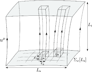
Figure 3: Time evolution of material particles in the large region $\Sigma_{x}[L_{\mathrm{s}}]$ [13].

We then consider the total entropy of the region $\Sigma_{x}[L_{\mathrm{s}}]$ :

$${\hat{S}}(t;\,\Sigma_{x}[L_{\mathrm{s}}])\equiv\int_{\Sigma_{x}[L_{\mathrm{s}}]}{\mathrm{d}}^{D}{\mathbf{y}}\,{\tilde{s}}\bigl{(}b^{A}(t,{\mathbf{y}}),\,{\tilde{c}}^{I}(t,{\mathbf{y}}),\,d^{P}(t,{\mathbf{y}})\bigr{)}\,.$$ (A.1)

The irreversible evolutions of intrinsic variables $a^{r}(x)\equiv\bigl{(}b^{A}(x),\,{\tilde{c}}^{I}(x)\bigr{)}$ at $x$ will proceed toward an equilibrium of the region $\Sigma_{x}[L_{\mathrm{s}}]$ . Due to the condition $L_{\mathrm{s}}\gg\epsilon_{\mathrm{s}}$ , we can assume that the influence from the surroundings of the region $\Sigma_{x}[L_{\mathrm{s}}]$ is not relevant to the dynamics of $a^{r}(x)$ because $x$ is well inside the region. An equilibrium state of the region $\Sigma_{x}[L_{\mathrm{s}}]$ will be realized when the observation is made for a long period of time, $L_{\mathrm{t}}$ , and can be characterized by the condition

$$\frac{\delta{\hat{S}}(t;\,\Sigma_{x}[L_{\mathrm{s}}])}{\delta a^{r}(x)}=0\,.$$ (A.2)

Note that the functional derivative is taken only with respect to a spatial, $D$-dimensional unit in the functional. We denote the values of $a^{r}(x)$ at the equilibrium by $a^{r}_{0}(x;\,L_{\mathrm{s}})\equiv\bigl{(}b^{A}_{0}(x;\,L_{\mathrm{s}}),\,{\tilde{c}}^{I}_{0}(x;\,L_{\mathrm{s}})\bigr{)}$ . One should note here that, since ${\tilde{c}}^{I}(t,{\mathbf{y}})$ are conserved quantities, the variations (A.2) with respect to ${\tilde{c}}^{I}$-type variables should be taken with total charges kept fixed at prescribed values:

$$\int_{\Sigma_{x}[L_{\mathrm{s}}]}{\mathrm{d}}^{D}{\mathbf{y}}\,{\tilde{c}}^{I}(t,{\mathbf{y}})\equiv C^{I}\bigl{(}\Sigma_{x}[L_{\mathrm{s}}]\bigr{)}\,.$$ (A.3)

A simple analysis using the Lagrange multipliers shows that the condition of global equilibrium is expressed locally as

$$\frac{\partial{\tilde{s}}}{\partial b^{A}}(x)=0\qquad\text{and}\qquad h_{\mu}^{~{}\nu}(x)\,\nabla_{\nu}\beta_{I}(x)=0\,,$$ (A.4)

where $\beta_{I}$ is the thermodynamic variable conjugate to ${\tilde{c}}^{I}$ that is defined by

$$\beta_{I}(x)\equiv\frac{\partial{\tilde{s}}}{\partial{\tilde{c}}^{I}}(x)\,.$$ (A.5)

The total entropy of the region $\Sigma_{x}[L_{\mathrm{s}}]$ at an equilibrium is given by

$${\hat{S}}_{0}(t;\,\Sigma_{x}[L_{\mathrm{s}}])\equiv\int_{\Sigma^{0}_{x}[L_{\mathrm{s}}]}{\mathrm{d}}^{D}{\mathbf{y}}\,{\tilde{s}}\bigl{(}b^{A}_{0}(t,{\mathbf{y}}),\,{\tilde{c}}^{I}_{0}(t,{\mathbf{y}}),\,d^{P}(t,{\mathbf{y}})\bigr{)}\,,$$ (A.6)

where $\Sigma^{0}_{x}[L_{\mathrm{s}}]$ is a hypersurface orthogonal to the velocity field at the equilibrium, $u_{0}^{\mu}\equiv p^{\mu}_{0}/e_{0}$ . When the material can be regarded as being at an equilibrium at spatial infinity, we can fix the labeling $s$ of the new timeslices $\{\Sigma^{0}_{s}\}$ at the equilibrium with the labeling $t$ of the original timeslices $\{\Sigma_{t}\}$ by setting $s=t$ if $\Sigma^{0}_{s}$ conforms with $\Sigma_{t}$ at spatial infinity. If we denote coordinates corresponding to the new foliation $\{\Sigma^{0}_{t}\}$ by $(x^{\prime\,\mu})=(x^{\prime\,0}=t\,,\,x^{\prime\,i})$, then the velocity field $u_{0}=u_{0}^{\mu}\,\partial^{\,\prime}_{\mu}$ will be expressed in the following form:

$$u_{0}=\frac{1}{N_{0}}\,\partial_{t}+\frac{1}{N^{i}_{0}}\,\partial^{\,\prime}_{i}\,.$$ (A.7)

This expression defines the new lapse $N_{0}$ and the new shifts $N_{0}^{i}$ at the equilibrium that are realized at spacetime scale $(L_{\rm s},L_{\rm t})$. For configurations other than the equilibrium, the total entropy ${\hat{S}}(t;\,\Sigma_{x}[L_{\mathrm{s}}])$ is smaller than that of the equilibrium ${\hat{S}}_{0}(t;\,\Sigma_{x}[L_{\mathrm{s}}])$ , so that if we denote their difference by

$$\Delta{\hat{S}}(t;\,\Sigma_{x}[L_{\mathrm{s}}])\equiv{\hat{S}}(t;\,\Sigma_{x}[L_{\mathrm{s}}])-{\hat{S}}_{0}(t;\,\Sigma_{x}[L_{\mathrm{s}}])\,,$$ (A.8)

$\Delta{\hat{S}}$ is always nonpositive.

In the previous paper [13], it is proposed that the difference $\Delta{\hat{S}}$ can be effectively written in the following form at the lowest order in the derivative expansion for linear nonequilibrium thermodynamics:

$$\Delta{\hat{S}}(t;\,\Sigma_{x}[L_{\mathrm{s}}])$$

$$=-\,\frac{1}{2}\,\int_{\Sigma^{0}_{x}[L_{\mathrm{s}}]}{\mathrm{d}}^{D}{\mathbf{y}}\,N_{0}^{-1}\,\sqrt{-g}\,\begin{pmatrix}(b-b_{0})^{A}&\nabla_{\mu}\beta_{I}\end{pmatrix}\begin{pmatrix}\ell_{AB}&\ell_{A}^{\,\nu J}\cr\ell_{B}^{\,\mu I}&\ell^{\,\mu I,\,\nu J}\end{pmatrix}\begin{pmatrix}(b-b_{0})^{B}\cr\nabla_{\nu}\beta_{J}\end{pmatrix}\,.$$ (A.9)

Here the scalar function $N_{0}$ is the lapse at the equilibrium defined in Eq. (A.7), the coefficient $\Bigl{(}\begin{smallmatrix}\ell_{AB}&\ell_{A}^{\,\nu J}\cr\ell_{B}^{\,\mu I}&\ell^{\,\mu I,\,\nu J}\end{smallmatrix}\Bigr{)}$ is a symmetric, positive semidefinite matrix, and all the elements are spatial tensors, $\ell_{A}^{\,\mu I}\,u_{\mu}=0=\ell^{\,\mu I,\,\nu J}\,u_{\nu}$ . The integral region can be replaced by $\Sigma_{x}[L_{\mathrm{s}}]$ because the difference is of higher orders in the derivative expansion. See the appendix in [13] for a derivation of (A.9) for simple cases. The functional form of the total entropy, ${\hat{S}}(t;\,\Sigma_{x}[L_{\mathrm{s}}])={\hat{S}}_{0}(t;\,\Sigma_{x}[L_{\mathrm{s}}])+\Delta{\hat{S}}(t;\,\Sigma_{x}[L_{\mathrm{s}}])$ , is called the entropy functional in [13].

We now consider Onsager’s linear regression theory [9, 10, 11, 12] assuming that the total entropy is given with this entropy functional. In Onsager’s treatment the irreversible evolutions of thermodynamic variables $a^{r}(x)$ are given by

$$[\dot{a}^{r}(x)]_{\mathrm{irr}}=L^{rs}\,f_{s}(x)\,.$$ (A.10)

Here $f_{s}(x)$ is the thermodynamic force defined by

$$f_{s}(x)=\frac{\delta\,\Delta{\hat{S}}(t;\,\Sigma_{x}[L_{\mathrm{s}}])}{\delta a^{s}(x)}\,,$$ (A.11)

and in the relativistic nonlinear thermodynamics, the dot should be defined as $\dot{a}^{r}\equiv N\,\pounds_{u}a^{r}$ [13], where $\pounds_{u}$ is the Lie derivative with respect to the velocity $u=u^{\mu}(x)\,\partial_{\mu}$ . $L^{rs}$ are the so-called phenomenological coefficients and can be shown to satisfy Onsager’s reciprocal relation [9, 10, 11]

$$L^{rs}=(-1)^{|a^{r}|+|a^{s}|}\,L^{sr}\,,$$ (A.12)

where the index $|a^{r}|$ expresses how the variables transform under time reversal, $a^{r}(x)\to(-1)^{|a^{r}|}\,a^{r}(x)$ . The Curie principle says that $L^{rs}$ can be block diagonalized with respect to the transformation properties of the indices $(r,s)$ under spatial rotations and the parity transformation [21], that is, under the subgroup $\mathrm{O}(D)$ of the local Lorentz group $\mathrm{O}(D,1)$ in local inertial frames. For example, when $a^{r}$ constitute a contravariant vector, $(a^{r})\equiv(a^{\mu})$ , the equations of linear regression should be set for each of the normal and tangential components to the timeslice through $x$ :

$$[\dot{a}(x)]_{{\mathrm{irr}}\,\bot}^{\mu}(x) =L_{\bot}^{\mu\nu}\,\biggl{[}\frac{\delta\,\Delta{\hat{S}}}{\delta a^{\nu}(x)}\biggr{]}_{\mbox{\raisebox{4.0pt}{\scriptsize{$\bot$}}}}\,,$$ (A.13)

$$[\dot{a}(x)]_{{\mathrm{irr}}\,\|}^{\mu}(x) =L_{\|}^{\mu\nu}\,\biggl{[}\frac{\delta\,\Delta{\hat{S}}}{\delta a^{\nu}(x)}\biggr{]}_{\mbox{\raisebox{4.0pt}{\scriptsize{$\|$}}}}\,,$$ (A.14)

where for a contravariant vector $v^{\mu}$ we define $v_{\bot}^{\mu}\equiv(-u^{\mu}u_{\nu})\,v^{\nu}$ and $v_{\|}^{\mu}\equiv h^{\mu}_{~{}\nu}\,v^{\nu}$ (and similarly for covariant vectors). Covariance and positivity further impose the condition that $L_{\bot}^{\mu\nu}$ and $L_{\|}^{\mu\nu}$ should be expressed as $L_{\bot}^{\mu\nu}=L_{\bot}\,u^{\mu}u^{\nu}$ $(L_{\bot}>0)$ and $L_{\|}^{\mu\nu}=L_{\|}\,h^{\mu\nu}$ $(L_{\|}>0)$ , respectively.

If we further know the reversible evolutions of thermodynamic variables, $[\dot{a}^{r}(x)]_{\mathrm{rev}}$ , which are not accompanied by entropy productions, then the dynamics of the system can be determined as

$$\dot{a}^{r}(x)=[\dot{a}^{r}(x)]_{\mathrm{rev}}+[\dot{a}^{r}(x)]_{\mathrm{irr}}=[\dot{a}^{r}(x)]_{\mathrm{rev}}+L^{rs}\,\frac{\delta\,\Delta{\hat{S}}(t;\,\Sigma_{x}[L_{\mathrm{s}}])}{\delta a^{s}(x)}\,.$$ (A.15)

For viscoelastic materials, the relevant thermodynamic variables are the following:

$b^{A}$	$b^{A}_{0}$	${\tilde{c}}^{I}$	$\beta_{I}$	$d^{P}$	$(\partial{\tilde{s}}/\partial d^{P})$
$\varepsilon_{\mu\nu}$	$0$	${\tilde{p}}_{\mu}$	$-u^{\mu}/T$	$g_{\mu\nu}$	$\sqrt{h}\,T_{\mathrm{(q)}}^{\mu\nu}/2T$
$\varepsilon_{\mu}$	$0$	${\tilde{n}}$	$-\mu/T$
$\theta$	$0$

where $T^{\mu\nu}_{\mathrm{(q)}}\equiv e\,u^{\mu}\,u^{\nu}+\tau_{\mathrm{(q)}}^{\mu\nu}$ is the quasiconservative energy-momentum tensor with $\tau_{\mathrm{(q)}}^{\mu\nu}$ the quasiconservative stress tensor. The entropy functional is then written as

$$\,\Delta{\hat{S}} (t;\,\Sigma_{x}[L_{\mathrm{s}}])$$

$$=-\frac{1}{2}\int_{\Sigma^{0}_{x}[L_{\mathrm{s}}]}\!\!\!{\mathrm{d}}^{D}{\mathbf{y}}\,\sqrt{-g}\,N_{0}^{-1}\,\times$$

$$\qquad\qquad\times\Biggl{[}\begin{pmatrix}\varepsilon_{\langle\mu\nu\rangle}&\nabla^{\langle\mu}\bigl{(}\partial{\tilde{s}}/\partial{\tilde{p}}_{\nu\rangle}\bigr{)}\end{pmatrix}\begin{pmatrix}\ell_{1}^{\langle\mu\nu\rangle,\langle\rho\sigma\rangle}&\ell^{\langle\mu\nu\rangle,}_{2~{}~{}~{}\langle\rho\sigma\rangle}\cr\ell_{2\,\langle\mu\nu\rangle,}^{~{}~{}~{}~{}~{}\langle\rho\sigma\rangle}&\ell_{3\,\langle\mu\nu\rangle,\langle\rho\sigma\rangle}\end{pmatrix}\begin{pmatrix}\varepsilon_{\langle\rho\sigma\rangle}\cr\nabla^{\langle\rho}\bigl{(}\partial{\tilde{s}}/\partial{\tilde{p}}_{\sigma\rangle}\bigr{)}\end{pmatrix}$$

$$\qquad\qquad\qquad+\begin{pmatrix}\varepsilon_{\mu}&\partial_{\mu}\bigl{(}\partial{\tilde{s}}/\partial{\tilde{n}}\bigr{)}\end{pmatrix}\begin{pmatrix}\ell_{1}^{\mu\nu}&\ell_{2}^{\mu\nu}\cr\ell_{2}^{\mu\nu}&\ell_{3}^{\mu\nu}\end{pmatrix}\begin{pmatrix}\varepsilon_{\nu}\cr\partial_{\nu}\bigl{(}\partial{\tilde{s}}/\partial{\tilde{n}}\bigr{)}\end{pmatrix}$$

$$\qquad\qquad\qquad+\begin{pmatrix}\operatorname{tr}\varepsilon&\theta&\nabla_{\mu}\bigl{(}\partial{\tilde{s}}/\partial{\tilde{p}}_{\mu}\bigr{)}\end{pmatrix}\begin{pmatrix}\hat{\ell}^{\mathrm{s}}_{1}&\hat{\ell}^{\mathrm{s}}_{2}&\hat{\ell}^{\mathrm{s}}_{4}\cr\hat{\ell}^{\mathrm{s}}_{2}&\hat{\ell}^{\mathrm{s}}_{3}&\hat{\ell}^{\mathrm{s}}_{5}\cr\hat{\ell}^{\mathrm{s}}_{4}&\hat{\ell}^{\mathrm{s}}_{5}&\hat{\ell}^{\mathrm{s}}_{6}\end{pmatrix}\begin{pmatrix}\operatorname{tr}\varepsilon\cr\theta\cr\nabla_{\mu}\bigl{(}\partial{\tilde{s}}/\partial{\tilde{p}}_{\mu}\bigr{)}\end{pmatrix}\Biggr{]}\,,$$

$$=-\frac{1}{2}\int_{\Sigma^{0}_{x}[L_{\mathrm{s}}]}\!\!\!{\mathrm{d}}^{D}{\mathbf{y}}\,\sqrt{-g}\,N_{0}^{-1}\,\times$$

$$\qquad\qquad\times\Biggl{[}\begin{pmatrix}\varepsilon_{\langle\mu\nu\rangle}&(-1/T)\,K_{\langle\mu\nu\rangle}\end{pmatrix}\begin{pmatrix}\ell_{1}^{\langle\mu\nu\rangle,\langle\rho\sigma\rangle}&\ell^{\langle\mu\nu\rangle,}_{2~{}~{}~{}\langle\rho\sigma\rangle}\cr\ell_{2\,\langle\mu\nu\rangle,}^{~{}~{}~{}~{}~{}\langle\rho\sigma\rangle}&\ell_{3\,\langle\mu\nu\rangle,\langle\rho\sigma\rangle}\end{pmatrix}\begin{pmatrix}\varepsilon_{\langle\rho\sigma\rangle}\cr(-1/T)\,K_{\langle\rho\sigma\rangle}\end{pmatrix}$$

$$\qquad\qquad\qquad+\begin{pmatrix}\varepsilon_{\mu}&\partial_{\mu}(-\mu/T)\end{pmatrix}\begin{pmatrix}\ell_{1}^{\mu\nu}&\ell_{2}^{\mu\nu}\cr\ell_{2}^{\mu\nu}&\ell_{3}^{\mu\nu}\end{pmatrix}\begin{pmatrix}\varepsilon_{\nu}\cr\partial_{\nu}(-\mu/T)\end{pmatrix}$$

$$\qquad\qquad\qquad+\begin{pmatrix}\operatorname{tr}\varepsilon&\theta&(-1/T)\,\operatorname{tr}K\end{pmatrix}\begin{pmatrix}\hat{\ell}^{\mathrm{s}}_{1}&\hat{\ell}^{\mathrm{s}}_{2}&\hat{\ell}^{\mathrm{s}}_{4}\cr\hat{\ell}^{\mathrm{s}}_{2}&\hat{\ell}^{\mathrm{s}}_{3}&\hat{\ell}^{\mathrm{s}}_{5}\cr\hat{\ell}^{\mathrm{s}}_{4}&\hat{\ell}^{\mathrm{s}}_{5}&\hat{\ell}^{\mathrm{s}}_{6}\end{pmatrix}\begin{pmatrix}\operatorname{tr}\varepsilon\cr\theta\cr(-1/T)\,\operatorname{tr}K\end{pmatrix}\Biggr{]}\,,$$ (A.16)

where the coefficient matrices are symmetric and positive semidefinite, and their indices are all orthogonal to $u^{\mu}$ . Note that for this parametrization, the contributions from the rotation $\nabla_{[\mu}u_{\nu]}$ are discarded. Since the matrices must be invariant tensors, we can assume that they take the following form:

$$\begin{pmatrix}\ell_{1}^{\langle\mu\nu\rangle,\langle\rho\sigma\rangle}&\ell_{2}^{\langle\mu\nu\rangle,\langle\rho\sigma\rangle}\cr\ell_{2}^{\langle\mu\nu\rangle,\langle\rho\sigma\rangle}&\ell_{3}^{\langle\mu\nu\rangle,\langle\rho\sigma\rangle}\end{pmatrix} =2\,\begin{pmatrix}\ell_{1}^{\mathrm{t}}&\ell_{2}^{\mathrm{t}}\cr\ell_{2}^{\mathrm{t}}&\ell_{3}^{\mathrm{t}}\end{pmatrix}\,N_{0}\,h^{\langle\mu}_{\mu^{\prime}}\,h^{\nu\rangle}_{\nu^{\prime}}\,h^{\mu^{\prime}\rho}\,h^{\nu^{\prime}\sigma}\,,$$ (A.17)

$$\begin{pmatrix}\ell_{1}^{\mu\nu}&\ell_{2}^{\mu\nu}\cr\ell_{2}^{\mu\nu}&\ell_{3}^{\mu\nu}\end{pmatrix} =\begin{pmatrix}\ell_{1}^{\mathrm{v}}&\ell_{2}^{\mathrm{v}}\cr\ell_{2}^{\mathrm{v}}&\ell_{3}^{\mathrm{v}}\end{pmatrix}\,N_{0}\,h^{\mu\nu}\,,$$ (A.18)

$$\begin{pmatrix}\hat{\ell}^{\mathrm{s}}_{1}&\hat{\ell}^{\mathrm{s}}_{2}&\hat{\ell}^{\mathrm{s}}_{4}\cr\hat{\ell}^{\mathrm{s}}_{2}&\hat{\ell}^{\mathrm{s}}_{3}&\hat{\ell}^{\mathrm{s}}_{5}\cr\hat{\ell}^{\mathrm{s}}_{4}&\hat{\ell}^{\mathrm{s}}_{5}&\hat{\ell}^{\mathrm{s}}_{6}\end{pmatrix} =\begin{pmatrix}\ell^{\mathrm{s}}_{1}&\ell^{\mathrm{s}}_{2}&\ell^{\mathrm{s}}_{4}\cr\ell^{\mathrm{s}}_{2}&\ell^{\mathrm{s}}_{3}&\ell^{\mathrm{s}}_{5}\cr\ell^{\mathrm{s}}_{4}&\ell^{\mathrm{s}}_{5}&\ell^{\mathrm{s}}_{6}\end{pmatrix}\,N_{0}\,,$$ (A.19)

where $\Bigl{(}\begin{smallmatrix}\ell_{1}^{\mathrm{t}}&\ell_{2}^{\mathrm{t}}\cr\ell_{2}^{\mathrm{t}}&\ell_{3}^{\mathrm{t}}\end{smallmatrix}\Bigr{)}$ , $\Bigl{(}\begin{smallmatrix}\ell_{1}^{\mathrm{v}}&\ell_{2}^{\mathrm{v}}\cr\ell_{2}^{\mathrm{v}}&\ell_{3}^{\mathrm{v}}\end{smallmatrix}\Bigr{)}$ and $\Bigl{(}\begin{smallmatrix}\ell^{\mathrm{s}}_{1}&\ell^{\mathrm{s}}_{2}&\ell^{\mathrm{s}}_{4}\cr\ell^{\mathrm{s}}_{2}&\ell^{\mathrm{s}}_{3}&\ell^{\mathrm{s}}_{5}\cr\ell^{\mathrm{s}}_{4}&\ell^{\mathrm{s}}_{5}&\ell^{\mathrm{s}}_{6}\end{smallmatrix}\Bigr{)}$ are positive semidefinite. The irreversible evolutions of thermodynamic variables then become

$$\bigl{[}\dot{\varepsilon}_{\langle\mu\nu\rangle}\bigr{]}_{\mathrm{irr}} \equiv\frac{1}{\sqrt{h}}\,L^{\varepsilon_{\langle\mu\nu\rangle}\varepsilon_{\langle\rho\sigma\rangle}}\,\frac{\delta\Delta{\hat{S}}}{\delta\varepsilon_{\rho\sigma}}\,,$$ (A.20)

$$\bigl{[}\dot{\varepsilon}_{\mu}\bigr{]}_{\mathrm{irr}\,\bot} \equiv\frac{1}{\sqrt{h}}\,L_{\bot}^{\varepsilon_{\mu}\varepsilon_{\nu}}\,\biggl{[}\frac{\delta\Delta{\hat{S}}}{\delta\varepsilon_{\nu}}\biggr{]}_{\mbox{\raisebox{3.0pt}{\scriptsize{$\bot$}}}}\equiv 0\,,$$ (A.21)

$$\bigl{[}\dot{\varepsilon}_{\mu}\bigr{]}_{\mathrm{irr}\,\|} \equiv\frac{1}{\sqrt{h}}\,L_{\|}^{\varepsilon_{\mu}\varepsilon_{\nu}}\,\biggl{[}\frac{\delta\Delta{\hat{S}}}{\delta\varepsilon_{\nu}}\biggr{]}_{\mbox{\raisebox{3.0pt}{\scriptsize{$\|$}}}}\,,$$ (A.22)

$$\begin{pmatrix}\bigl{[}(\operatorname{tr}\varepsilon)^{\cdot}\bigr{]}_{\mathrm{irr}}\cr\bigl{[}\,\dot{\theta}\,\bigr{]}_{\mathrm{irr}}\end{pmatrix} \equiv\frac{1}{\sqrt{h}}\,\begin{pmatrix}L^{\operatorname{tr}\varepsilon\,\operatorname{tr}\varepsilon}&L^{\operatorname{tr}\varepsilon\,\theta}\cr L^{\operatorname{tr}\varepsilon\,\theta}&L^{\theta\,\theta}\ \end{pmatrix}\begin{pmatrix}\delta\Delta{\hat{S}}/\delta(\operatorname{tr}\varepsilon)\cr\delta\Delta{\hat{S}}/\delta\theta\end{pmatrix}\,,$$ (A.23)

$$\bigl{[}\,\dot{\tilde{p}}_{\mu}\bigr{]}_{\mathrm{irr}\,\bot} \equiv\sqrt{h}\,L_{\bot}^{{\tilde{p}}_{\mu}{\tilde{p}}_{\nu}}\,\biggl{[}\frac{\delta\Delta{\hat{S}}}{\delta{\tilde{p}}_{\nu}}\biggr{]}_{\mbox{\raisebox{3.0pt}{\scriptsize{$\bot$}}}}\,,$$ (A.24)

$$\bigl{[}\,\dot{\tilde{p}}_{\mu}\bigr{]}_{\mathrm{irr}\,\|} \equiv\sqrt{h}\,L_{\|}^{{\tilde{p}}_{\mu}{\tilde{p}}_{\nu}}\,\biggl{[}\frac{\delta\Delta{\hat{S}}}{\delta{\tilde{p}}_{\nu}}\biggr{]}_{\mbox{\raisebox{3.0pt}{\scriptsize{$\|$}}}}\,,$$ (A.25)

$$[\dot{\tilde{n}}]_{\mathrm{irr}} \equiv\sqrt{h}\,L^{{\tilde{n}}{\tilde{n}}}\,\frac{\delta\Delta{\hat{S}}}{\delta{\tilde{n}}}\,.$$ (A.26)

We now make the following irreducible decompositions of the phenomenological constants under the group $\mathrm{O}(D)$ in a local inertial frame:

$$L^{\varepsilon_{\langle\mu\nu\rangle}\varepsilon_{\langle\rho\sigma\rangle}} \equiv L^{\mathrm{t}}\,h_{\langle\mu}^{\mu^{\prime}}h_{\nu\rangle}^{\nu^{\prime}}h_{\mu^{\prime}\rho}h_{\nu^{\prime}\sigma}\,,\qquad L_{\|}^{\varepsilon_{\mu}\varepsilon_{\nu}}\equiv L^{\mathrm{v}}\,h_{\mu\nu}\,,$$ (A.27)

$$L^{\operatorname{tr}\varepsilon\,\operatorname{tr}\varepsilon} \equiv L^{\mathrm{s}}_{1}\,,\qquad L^{\operatorname{tr}\varepsilon\,\theta}\equiv L^{\mathrm{s}}_{2}\,,\qquad L^{\theta\,\theta}\equiv L^{\mathrm{s}}_{3}\,,$$ (A.28)

$$L_{\bot}^{{\tilde{p}}_{\mu}{\tilde{p}}_{\nu}} \equiv L_{\bot}\,u_{\mu}u_{\nu}\,,\quad L_{\|}^{{\tilde{p}}_{\mu}{\tilde{p}}_{\nu}}\equiv L_{\|}\,h_{\mu\nu}\,,\quad L^{{\tilde{n}}{\tilde{n}}}\equiv M\,.$$ (A.29)

Then the irreversible evolutions of thermodynamic variables can be written as [13]

$$N^{-1}[\dot{\varepsilon}_{\langle\mu\nu\rangle}]_{\mathrm{irr}} =-2L^{\mathrm{t}}\ell_{1}^{\mathrm{t}}\,\varepsilon_{\langle\mu\nu\rangle}+(2L^{\mathrm{t}}\ell_{2}^{\mathrm{t}}/T)\,K_{\langle\mu\nu\rangle}\,,$$ (A.30)

$$N^{-1}\bigl{[}\dot{\varepsilon}_{\mu}\bigr{]}_{\mathrm{irr}} =-L^{\mathrm{v}}\,h_{\mu}^{~{}\nu}\,\bigl{[}\ell_{1}^{\mathrm{v}}\,\varepsilon_{\nu}+\ell_{2}^{\mathrm{v}}\,\partial_{\nu}(-\mu/T)\bigr{]}\,,$$ (A.31)

$$N^{-1}\bigl{[}(\operatorname{tr}\varepsilon)^{\cdot}\bigr{]}_{\mathrm{irr}} =-(L^{\mathrm{s}}_{1}\,\ell^{\mathrm{s}}_{1}+L^{\mathrm{s}}_{2}\,\ell^{\mathrm{s}}_{2})\,\operatorname{tr}\varepsilon-(L^{\mathrm{s}}_{1}\,\ell^{\mathrm{s}}_{2}+L^{\mathrm{s}}_{2}\,\ell^{\mathrm{s}}_{3})\,\theta+(L^{\mathrm{s}}_{1}\,\ell^{\mathrm{s}}_{4}+L^{\mathrm{s}}_{2}\,\ell^{\mathrm{s}}_{5})\,\frac{1}{T}\operatorname{tr}K\,,$$ (A.32)

$$N^{-1}\bigl{[}\,\dot{\theta}\,\bigr{]}_{\mathrm{irr}} =-\,(L^{\mathrm{s}}_{2}\,\ell^{\mathrm{s}}_{1}+L^{\mathrm{s}}_{3}\,\ell^{\mathrm{s}}_{2})\,\operatorname{tr}\varepsilon-(L^{\mathrm{s}}_{2}\,\ell^{\mathrm{s}}_{2}+L^{\mathrm{s}}_{3}\,\ell^{\mathrm{s}}_{3})\,\theta+(L^{\mathrm{s}}_{2}\,\ell^{\mathrm{s}}_{4}+L^{\mathrm{s}}_{3}\,\ell^{\mathrm{s}}_{5})\,\frac{1}{T}\operatorname{tr}K\,,$$ (A.33)

$$\frac{1}{\sqrt{-g}}\,\bigl{[}\,\dot{\tilde{p}}_{\nu}\bigr{]}_{\mathrm{irr}\,\bot} =-\,c_{\bot}\,L_{\bot}\,(-u_{\nu}u_{\lambda})\,\nabla_{\mu}\,\bigl{[}\,2\,\ell^{\mathrm{t}}_{2}\,\varepsilon^{\langle\mu\lambda\rangle}-(2/T)\,\ell^{\mathrm{t}}_{3}\,K^{\langle\mu\lambda\rangle}$$

$$\qquad\qquad\qquad\qquad\qquad\quad+\bigl{(}\ell^{\mathrm{s}}_{4}\,\operatorname{tr}\varepsilon+\ell^{\mathrm{s}}_{5}\,\theta-(1/T)\,\ell^{\mathrm{s}}_{6}\,\operatorname{tr}K\bigr{)}\,h^{\mu\lambda}\bigr{]}\,,$$ (A.34)

$$\frac{1}{\sqrt{-g}}\,\bigl{[}\,\dot{\tilde{p}}_{\nu}\bigr{]}_{\mathrm{irr}\,\|} =-\,c_{\|}\,L_{\|}\,h_{\nu\lambda}\,\nabla_{\mu}\,\bigl{[}\,2\,\ell^{\mathrm{t}}_{2}\,\varepsilon^{\langle\mu\lambda\rangle}-(2/T)\,\ell^{\mathrm{t}}_{3}\,K^{\langle\mu\lambda\rangle}$$

$$\qquad\qquad\qquad\qquad\qquad\quad+\bigl{(}\ell^{\mathrm{s}}_{4}\,\operatorname{tr}\varepsilon+\ell^{\mathrm{s}}_{5}\,\theta-(1/T)\,\ell^{\mathrm{s}}_{6}\,\operatorname{tr}K\bigr{)}\,h^{\mu\lambda}\bigr{]}\,,$$ (A.35)

$$\frac{1}{\sqrt{-g}}\,[\dot{\tilde{n}}]_{\mathrm{irr}} =-\,\sqrt{h}\,(-\partial^{2}{\tilde{s}}/\partial{\tilde{n}}^{2})\,M\,\nabla_{\mu}\,\bigl{[}\,\ell^{\mathrm{v}}_{2}\,h^{\mu\nu}\,\varepsilon_{\nu}+\ell^{\mathrm{v}}_{3}\,h^{\mu\nu}\,\partial_{\nu}(-\mu/T)\bigr{]}\,.$$ (A.36)

Here, in order to evaluate $\delta\Delta{\hat{S}}/\delta{\tilde{p}}_{\mu}$ , we have used the decomposition of the matrix $\partial^{2}{\tilde{s}}/\partial{\tilde{p}}_{\mu}\partial{\tilde{p}}_{\nu}$ (negative-definite for each irreducible component) as

$$\sqrt{h}\,\frac{\partial^{2}{\tilde{s}}}{\partial{\tilde{p}}_{\mu}\partial{\tilde{p}}_{\nu}}=-c_{\bot}\,u^{\mu}u^{\nu}-c_{\|}\,h^{\mu\nu}$$ (A.37)

with positive quantities $c_{\bot}$ and $c_{\|}$ .

If we assume that $L_{\tilde{p}}\equiv c_{\bot}L_{\bot}=c_{\|}L_{\|}$ and $L_{\tilde{n}}\equiv\sqrt{h}\,(-\partial^{2}{\tilde{s}}/\partial{\tilde{n}}^{2})\,M$ are constant, then Eqs. (A.34)–(A.36) are rewritten as

$$[\dot{{\tilde{p}}}_{\nu}]_{\mathrm{irr}}=-\,\sqrt{-g}\,\nabla^{\mu}\tau^{\mathrm{(d)}}_{\mu\nu}\,,\qquad[\dot{{\tilde{n}}}]_{\mathrm{irr}}=-\,\sqrt{-g}\,\nabla^{\mu}\nu^{\mathrm{(d)}}_{\mu}\,,$$ (A.38)

where the dissipation currents are given by

$$\tau^{\mathrm{(d)}}_{\mu\nu} \equiv L_{\tilde{p}}\,\bigl{[}\,2\,\ell^{\mathrm{t}}_{2}\,\varepsilon_{\langle\mu\nu\rangle}-(2/T)\,\ell^{\mathrm{t}}_{3}\,K_{\langle\mu\nu\rangle}+\bigl{(}\ell^{\mathrm{s}}_{4}\,\operatorname{tr}\varepsilon+\ell^{\mathrm{s}}_{5}\,\theta-(1/T)\,\ell^{\mathrm{s}}_{6}\,\operatorname{tr}K\bigr{)}\,h_{\mu\nu}\bigr{]}\,,$$ (A.39)

$$\nu^{\mathrm{(d)}}_{\mu} \equiv L_{\tilde{n}}\,\bigl{[}\,\ell^{\mathrm{v}}_{2}\,\varepsilon_{\mu}+\ell^{\mathrm{v}}_{3}\,h_{\mu}^{~{}\nu}\,\partial_{\nu}(-\mu/T)\bigr{]}\,.$$ (A.40)

On the other hand, as for the isentropic evolutions, we assume that the evolutions of the densities of conserved quantities are given by

$$[\dot{{\tilde{p}}}_{\nu}]_{\mathrm{rev}}=-\,\sqrt{-g}\,\nabla^{\mu}\tau^{\mathrm{(r)}}_{\mu\nu}\,,\qquad[\dot{{\tilde{n}}}]_{\mathrm{rev}}=-\,\sqrt{-g}\,\nabla^{\mu}\nu^{\mathrm{(r)}}_{\mu}$$ (A.41)

with the reversible currents of the following form:

$$\tau^{\mathrm{(r)}}_{\mu\nu} \equiv\tau^{\mathrm{(q)}}_{\mu\nu}-\,2\mathcal{G}\,\varepsilon_{\langle\mu\nu\rangle}-\mathcal{K}\,\bigl{(}\operatorname{tr}\varepsilon-a\,\theta)\,h_{\mu\nu}\,,$$ (A.42)

$$\nu^{\mathrm{(r)}}_{\mu} \equiv-\mathcal{H}\,\varepsilon_{\mu}\,.$$ (A.43)

As for the evolutions of the strains $E_{\mu\nu}=(\varepsilon_{\mu\nu}\,,\,\varepsilon_{\mu}\,,\,\theta)$ , we set them to be in the most generic form:

$$N^{-1}\bigl{[}\dot{\varepsilon}_{\langle\mu\nu\rangle}\bigr{]}_{\mathrm{rev}} =(2\mathcal{G}L^{\mathrm{t}}/L_{\tilde{p}}\,T)\,K_{\langle\mu\nu\rangle}\,,$$ (A.44)

$$N^{-1}\bigl{[}\dot{\varepsilon}_{\mu}\bigr{]}_{\mathrm{rev}} =-\,(L^{\mathrm{v}}\mathcal{H}/L_{\tilde{n}})\,h_{\mu}^{~{}\nu}\,\partial_{\nu}(-\mu/T)\,,$$ (A.45)

$$\begin{pmatrix}N^{-1}\bigl{[}(\operatorname{tr}\varepsilon)^{\cdot}\bigr{]}_{\mathrm{rev}}\cr N^{-1}\bigl{[}\,\dot{\theta}\,\bigr{]}_{\mathrm{rev}}\end{pmatrix} =-L_{\tilde{p}}^{-1}\,\begin{pmatrix}L^{\mathrm{s}}_{1}&L^{\mathrm{s}}_{2}\cr L^{\mathrm{s}}_{2}&L^{\mathrm{s}}_{3}\end{pmatrix}\begin{pmatrix}\mathcal{K}^{\prime}\,\theta-(\mathcal{K}/T)\,\operatorname{tr}K\cr-\mathcal{K}^{\prime}\operatorname{tr}\varepsilon+(\mathcal{K}/T)\,\operatorname{tr}K\end{pmatrix}\,.$$ (A.46)

Combining Eqs. (A.38)–(A.40) and Eqs. (A.41)–(A.43), and using the formulas $\dot{\tilde{p}}_{\nu}=\sqrt{-g}\,\nabla_{\mu}(u^{\mu}\,p_{\nu})=\sqrt{-g}\,\nabla^{\mu}(e\,u_{\mu}u_{\nu})$ and $\dot{\tilde{n}}=\sqrt{-g}\,\nabla^{\mu}(n\,u_{\mu})$ , we obtain

$$\sqrt{-g}\,\nabla^{\mu}(e\,u_{\mu}u_{\nu}) =\dot{{\tilde{p}}}_{\nu}=\bigl{[}\dot{{\tilde{p}}}_{\nu}\bigr{]}_{\mathrm{rev}}+\bigl{[}\dot{{\tilde{p}}}_{\nu}\bigr{]}_{\mathrm{irr}}=-\sqrt{-g}\,\nabla^{\mu}\bigl{(}\tau_{\mu\nu}^{\mathrm{(r)}}+\tau_{\mu\nu}^{\mathrm{(d)}}\bigr{)}\,,$$ (A.47)

$$\sqrt{-g}\,\nabla^{\mu}(n\,u_{\mu}) =\dot{{\tilde{n}}}=\bigl{[}\dot{{\tilde{n}}}\bigr{]}_{\mathrm{rev}}+\bigl{[}\dot{{\tilde{n}}}\bigr{]}_{\mathrm{irr}}=-\sqrt{-g}\,\nabla^{\mu}\bigl{(}\nu_{\mu}^{\mathrm{(r)}}+\nu_{\mu}^{\mathrm{(d)}}\bigr{)}\,.$$ (A.48)

We thus find that (A.34)–(A.36) [or Eqs. (A.38)–(A.40)] and Eqs. (A.41)–(A.43) can be summarized as current conservations:

$$\nabla_{\mu}T^{\mu\nu}=0\,,\qquad\nabla_{\mu}n^{\mu}=0\,,$$ (A.49)

where each of the conserved currents,

$$T^{\mu\nu}\equiv e\,u^{\mu}u^{\nu}+\tau^{\mu\nu}\,,\qquad n^{\mu}\equiv n\,u^{\mu}+\nu^{\mu}\,,$$ (A.50)

consists of the convective current ($p^{\nu}u^{\mu}=e\,u^{\mu}u^{\nu}$ or $nu^{\mu}$) and the additional current ($\tau^{\mu\nu}$ or $\nu^{\mu}$), the latter being further decomposed into the reversible and the dissipative currents:

$$\tau^{\mu\nu}\equiv\tau^{\mu\nu}_{\mathrm{(r)}}+\tau^{\mu\nu}_{\mathrm{(d)}}\,,\qquad\nu^{\mu}\equiv\nu^{\mu}_{\mathrm{(r)}}+\nu^{\mu}_{\mathrm{(d)}}\,.$$ (A.51)

Furthermore, one can easily show that the evolution equations on $E_{\mu\nu}=(\varepsilon_{\mu\nu}\,,\,\varepsilon_{\mu}\,,\,\theta)$ [Eqs. (A.30)–(A.33)] together with the explicit form of the reversible and the dissipative currents [Eqs. (A.39), (A.40), (A.42), and (A.43)] can be rewritten into the following set of equations:

$$\begin{pmatrix}-(2\lambda_{1}/T)\,\pounds_{u}\varepsilon_{\langle\mu\nu\rangle}\cr\tau_{\langle\mu\nu\rangle}-\tau^{(q)}_{\langle\mu\nu\rangle}\end{pmatrix} =2\,({\boldsymbol{\mathcal{G}}}+{\boldsymbol{\eta}})\begin{pmatrix}\varepsilon_{\langle\mu\nu\rangle}\cr-(1/T)\,K_{\langle\mu\nu\rangle}\end{pmatrix}\,,$$ (A.52)

$$\begin{pmatrix}-(\lambda_{2}/T)\,\pounds_{u}\varepsilon_{\mu}\cr\nu_{\mu}\end{pmatrix} =({\boldsymbol{\mathcal{H}}}+{\boldsymbol{\sigma}})\begin{pmatrix}\varepsilon_{\mu}\cr h_{\mu}^{~{}\nu}\partial_{\nu}(-\mu/T)\end{pmatrix}\,,$$ (A.53)

$$\begin{pmatrix}-(1/T)\,{\boldsymbol{\gamma}}\begin{pmatrix}\pounds_{u}(\operatorname{tr}\varepsilon)\cr\pounds_{u}\theta\end{pmatrix}\cr(1/D)\,(\operatorname{tr}\tau-\operatorname{tr}\tau_{\mathrm{(q)}})\end{pmatrix} =({\boldsymbol{\mathcal{K}}}+{\boldsymbol{\zeta}})\begin{pmatrix}\operatorname{tr}\varepsilon\cr\theta\cr(-1/T)\,\operatorname{tr}K\end{pmatrix}\,,$$ (A.54)

where

$$\lambda_{1} \equiv\frac{L_{{\tilde{p}}}\,T}{2L^{\mathrm{t}}}\,,\qquad\lambda_{2}\equiv\frac{L_{{\tilde{n}}}\,T}{L^{\mathrm{v}}}\,,\qquad{\boldsymbol{\gamma}}\equiv\begin{pmatrix}\gamma_{1}&\gamma_{2}\cr\gamma_{2}&\gamma_{3}\end{pmatrix}\equiv\Biggl{[}\frac{1}{L_{{\tilde{p}}}\,T}\,\begin{pmatrix}L^{\mathrm{s}}_{1}&L^{\mathrm{s}}_{2}\cr L^{\mathrm{s}}_{2}&L^{\mathrm{s}}_{3}\end{pmatrix}\Biggr{]}^{-1}\,,$$ (A.55)

$${\boldsymbol{\eta}} \equiv L_{{\tilde{p}}}\,\begin{pmatrix}\ell^{\mathrm{t}}_{1}&\ell^{\mathrm{t}}_{2}\cr\ell^{\mathrm{t}}_{2}&\ell^{\mathrm{t}}_{3}\end{pmatrix}\,,\quad{\boldsymbol{\sigma}}\equiv L_{{\tilde{n}}}\,\begin{pmatrix}\ell^{\mathrm{v}}_{1}&\ell^{\mathrm{v}}_{2}\cr\ell^{\mathrm{v}}_{2}&\ell^{\mathrm{v}}_{3}\end{pmatrix}\,,\quad{\boldsymbol{\zeta}}\equiv L_{{\tilde{p}}}\,\begin{pmatrix}\ell^{\mathrm{s}}_{1}&\ell^{\mathrm{s}}_{2}&\ell^{\mathrm{s}}_{4}\cr\ell^{\mathrm{s}}_{2}&\ell^{\mathrm{s}}_{3}&\ell^{\mathrm{s}}_{5}\cr\ell^{\mathrm{s}}_{4}&\ell^{\mathrm{s}}_{5}&\ell^{\mathrm{s}}_{6}\cr\end{pmatrix}\,,$$ (A.56)

$${\boldsymbol{\mathcal{G}}} \equiv\begin{pmatrix}0&\mathcal{G}\cr-\mathcal{G}&0\end{pmatrix}\,,\quad{\boldsymbol{\mathcal{H}}}\equiv\begin{pmatrix}0&\mathcal{H}\cr-\mathcal{H}&0\end{pmatrix}\,,\quad{\boldsymbol{\mathcal{K}}}\equiv\begin{pmatrix}0&\mathcal{K}^{\prime}&\mathcal{K}\cr-\mathcal{K}^{\prime}&0&-\mathcal{K}a\cr-\mathcal{K}&\mathcal{K}a&0\cr\end{pmatrix}\,.$$ (A.57)

Equations (A.52)–(A.57) totally agree with Eqs. (2.34)–(2.38), from which Eqs. (2.39)–(2.45) follow, as we see in Sec. 2.3. This is what we promised to show at the beginning of this Appendix.

We close this appendix with a comment on how the reversible evolutions are determined. They are actually determined by the requirement that the reversible evolutions do not produce entropy and the final form of the total evolutions (reversible ones plus irreversible ones) should be given as in Eqs. (A.52)–(A.57). As an example, let us consider the irreversible evolution of $\varepsilon_{\langle\mu\nu\rangle}$ and the quantity $\tau_{\langle\mu\nu\rangle}-\tau^{\mathrm{(q)}}_{\langle\mu\nu\rangle}$ :

$$N^{-1}\,\bigl{[}\dot{\varepsilon}_{\langle\mu\nu\rangle}\bigr{]}_{\mathrm{irr}} =-2L^{\mathrm{t}}\,\ell^{\mathrm{t}}_{1}\,\varepsilon_{\langle\mu\nu\rangle}+\frac{2L^{\mathrm{t}}\,\ell^{\mathrm{t}}_{2}}{T}\,K_{\langle\mu\nu\rangle}\,,$$ (A.58)

$$\tau_{\langle\mu\nu\rangle}-\tau^{\mathrm{(q)}}_{\langle\mu\nu\rangle} =-2\mathcal{G}\,\varepsilon_{\langle\mu\nu\rangle}+2L_{\tilde{p}}\,\ell^{\mathrm{t}}_{2}\,\varepsilon_{\langle\mu\nu\rangle}-\frac{2L_{\tilde{p}}\,\ell^{\mathrm{t}}_{3}}{T}\,K_{\langle\mu\nu\rangle}\,.$$ (A.59)

By multiplying the first equation by a factor $-L_{\tilde{p}}/L^{\mathrm{t}}$ , the equations can be rewritten with a symmetric matrix as

$$\begin{pmatrix}-(L_{\tilde{p}}/L^{\mathrm{t}})\,N^{-1}\,\bigl{[}\dot{\varepsilon}_{\langle\mu\nu\rangle}\bigr{]}_{\mathrm{irr}}\cr\tau_{\langle\mu\nu\rangle}-\tau^{\mathrm{(q)}}_{\langle\mu\nu\rangle}\end{pmatrix}=\left[\begin{pmatrix}0&0\cr-2\mathcal{G}&0\end{pmatrix}+2L_{\tilde{p}}\begin{pmatrix}\ell^{\mathrm{t}}_{1}&\ell^{\mathrm{t}}_{2}\cr\ell^{\mathrm{t}}_{2}&\ell^{\mathrm{t}}_{3}\end{pmatrix}\right]\begin{pmatrix}\varepsilon_{\langle\mu\nu\rangle}\cr-(1/T)\,K_{\langle\mu\nu\rangle}\end{pmatrix}\,.$$ (A.60)

The second term with a symmetric positive-semidefinite matrix represents irreversible processes with entropy production. Thus, in order for the first term not to produce entropy, we need to introduce the reversible part in $\dot{\varepsilon}_{\langle\mu\nu\rangle}$ such that the resulting form can be written with an antisymmetric matrix. This consideration determines the reversible evolution uniquely as

$$\begin{pmatrix}-(L_{\tilde{p}}/L^{\mathrm{t}})\,N^{-1}\,\bigl{[}\dot{\varepsilon}_{\langle\mu\nu\rangle}\bigr{]}_{\mathrm{rev}}\cr 0\end{pmatrix}=\begin{pmatrix}0&2\mathcal{G}\cr 0&0\end{pmatrix}\begin{pmatrix}\varepsilon_{\langle\mu\nu\rangle}\cr-(1/T)\,K_{\langle\mu\nu\rangle}\end{pmatrix}\,.$$ (A.61)

Noting that $N^{-1}\,\dot{\varepsilon}_{\langle\mu\nu\rangle}=\pounds_{u}\varepsilon_{\langle\mu\nu\rangle}$ , we see that the total evolution is actually given as in (A.52). The remaining equations can be obtained in a similar way.

Appendix B Constitutive equations in rheological models

The theory of elasticity is based on Hooke’s law which states that that stresses are proportional to strains in elastic materials. On the other hand, the theory of viscous fluids is based on Newton’s law which states that viscous stresses are proportional to velocity gradients in fluids, and is described by the Navier-Stokes equations. However, for more general materials these theories are not applicable, and a class of such materials is called viscoelastic materials and studied in the area of rheology. The relation between stresses and strains for a given material is called the constitutive equations, which play a fundamental role in the study of rheology. In this Appendix, we list a few well-known materials with their constitutive equations and compare them with the viscoelastic materials discussed in the bulk of the present paper.

Hookean materials

The simplest constitutive equations constitute Hooke’s law. We first assume that, on each timeslice $\Sigma_{t}$ , every material particle knows its own natural shape described by the reference metric $\bar{h}_{\mu\nu}$ , which measures distances in a material when it is free of elastic strains. This metric has the same meaning as the intrinsic metric in the main text, though it is not dynamical here ($\pounds_{u}\bar{h}_{\mu\nu}=0$) . When we discuss nonrelativistic dynamics, we will set it to be $\bar{h}_{\mu\nu}=\mathrm{diag}(0,1,\dotsc,1)$ in a laboratory frame, as is taken in standard textbooks (e.g., [5]). Although we consider the strain tensor $E_{\mu\nu}$ in the main text, we here assume that elastic strains are purely spatial, and only consider the elastic strain tensor defined by $\varepsilon_{\mu\nu}\equiv(1/2)\,(h_{\mu\nu}-\bar{h}_{\mu\nu})$ .

Hooke’s law can then be expressed as

$$\tau^{\mu\nu}=-\mathcal{K}^{(\mu\nu)(\rho\sigma)}\,\varepsilon_{\rho\sigma}\qquad(\mathcal{K}^{(\mu\nu)(\rho\sigma)}\geq 0)\,,$$ (B.1)

where $\mathcal{K}^{(\mu\nu)(\rho\sigma)}$ is a constant tensor, and $(~{})$ denotes the symmetrization of indices with the normalization $((~{}))=(~{})$ . For isotropic elastic materials which locally has no preferred direction, the coefficient $\mathcal{K}^{(\mu\nu)(\rho\sigma)}$ can be expressed as the sum of the irreducible components $h^{\mu\nu}\,h^{\rho\sigma}$ and $(1/2)\,\bigl{(}h^{\mu\rho}\,h^{\nu\sigma}+h^{\mu\sigma}\,h^{\nu\rho}-(2/D)\,h^{\mu\nu}\,h^{\rho\sigma}\bigr{)}$ , and we have

$$\tau_{\mu\nu}=-\mathcal{K}\,(\operatorname{tr}\varepsilon)\,h_{\mu\nu}-2\mathcal{G}\,\varepsilon_{\langle\mu\nu\rangle}\,,$$ (B.2)

where $\mathcal{K}$ and $\mathcal{G}$ are the bulk and the shear modulus, respectively. Relativistic motions of such elastic materials in gravitational fields are discussed in, e.g., [15].

Since we are considering the linear approximation in $\varepsilon_{\mu\nu}$ , this stress tensor can also be written as

$$\tau_{\mu\nu}=-\mathcal{K}\,(\overline{\operatorname{tr}}\varepsilon)\,\bar{h}_{\mu\nu}-2\mathcal{G}\,\varepsilon_{\overline{\langle\mu\nu\rangle}}\,,$$ (B.3)

where $\overline{\operatorname{tr}}$ and $\varepsilon_{\overline{\langle\mu\nu\rangle}}$ are defined by

$$\overline{\operatorname{tr}}\varepsilon=\varepsilon_{\mu\nu}\,\bar{h}^{\mu\nu}\,,\qquad\varepsilon_{\overline{\langle\mu\nu\rangle}}=\varepsilon_{\mu\nu}-\frac{1}{D}\,(\overline{\operatorname{tr}}\varepsilon)\,\bar{h}_{\mu\nu}\,.$$ (B.4)

Then, if we take the nonrelativistic approximation with $\bar{h}_{\mu\nu}=\mathrm{diag}(0,1,\dotsc,1)$ , we reproduce the standard Hookean stress tensor

$$\tau_{ij}=-\mathcal{K}\,\bigl{(}\delta^{kl}\,\varepsilon_{kl}\bigr{)}\,\delta_{ij}-2\mathcal{G}\,\Bigl{(}\varepsilon_{ij}-\frac{1}{D}\,\bigl{(}\delta^{kl}\,\varepsilon_{kl}\bigr{)}\delta_{ij}\Bigr{)}\,.$$ (B.5)

The constitutive equations for a Hookean material are schematically represented by a spring, as depicted in Fig. 4.

Figure 4: The bulk part (left) and shear part (right) for a Hookean material.

To understand the diagram, we consider a Hookean material in $D=1$ spatial dimension. The material can be obtained by connecting in series tiny springs with a weight of mass $m$ at each end (see Fig. 5).

Figure 5: Weights of mass $m$ are connected to the spring with spring constant $k$ .

Since the actual length between two adjacent weights at $x=x_{n}\equiv n\,l$ ($n\in\mathbb{Z}$) and $x=x_{n+1}$ is given by $\sqrt{h_{11}(x_{n})}\,l$ , and since the natural length is given by $\sqrt{\bar{h}_{11}(x_{n})}\,l$ , the stretch of the spring is given by $(\sqrt{h_{11}}-\sqrt{\bar{h}_{11}})\,l\simeq(\varepsilon_{11}/\sqrt{\bar{h}_{11}})\,(x_{n})$ , where $\varepsilon_{11}=(1/2)\,(h_{11}-\bar{h}_{11})$. Then the equation of motion for the weight at $x=x_{n}$ can be written as

$$m\,a_{1}(x_{n})=-k\,l\,\frac{\varepsilon_{11}}{\sqrt{\bar{h}_{11}}}(x_{n-1})+k\,l\,\frac{\varepsilon_{11}}{\sqrt{\bar{h}_{11}}}(x_{n})\,,$$ (B.6)

where $a_{1}(x_{n})$ is the acceleration of the weight at $x=x_{n}$ in the $x^{1}$-direction. Then in the continuum limit $l\to 0$ with $e_{0}\equiv m/\sqrt{\bar{h}_{11}}\,l$ and $\mathcal{K}\equiv k\,l$ kept fixed at finite values, the equation becomes

$$e_{0}\,a_{1}(x)=-\partial_{1}\bigl{[}-\mathcal{K}\,\bigl{(}\overline{\operatorname{tr}}\varepsilon(x)\bigl{)}\,\delta^{1}_{~{}1}\bigr{]}\,,$$ (B.7)

so long as we take a coordinate system in which the intrinsic metric $\bar{h}_{11}$ is spatially constant. If we define the energy density $e(x)\equiv m/\sqrt{h_{11}}\,l$ and neglect the difference $(e(x)-e_{0})\,a_{1}(x)$ , which is of higher orders in $\varepsilon_{11}$ , we obtain the Euler equation

$$e(x)\,a_{1}(x)=-\partial_{1}\tau^{1}_{~{}1}$$ (B.8)

with the stress tensor $\tau^{1}_{~{}1}=-\mathcal{K}\,(\overline{\operatorname{tr}}\varepsilon)\,\delta^{1}_{~{}1}$ . This stress tensor coincides with (B.3) in $D=1$ dimension, and in this sense the left diagram in Fig. 4 represents (the bulk part of) the constitutive equations for a Hookean material. On the other hand, the right diagram in Fig. 4 is simply a schematic generalization for the shear part and does not have any physical meaning other than the information that the shear part of the stress tensor is given by $-2\mathcal{G}\,\varepsilon_{\langle\mu\nu\rangle}$ .

Navier-Stokes (Newtonian) fluids

Newton’s viscosity law says that the viscous stress tensor is proportional to velocity gradients, and in our notations this can be written as

$$\tau_{\mathrm{(d)}}^{\mu\nu}=-\zeta^{(\mu\nu)(\rho\sigma)}K_{\rho\sigma}\qquad(\zeta^{(\mu\nu)(\rho\sigma)}\geq 0)\,,$$ (B.9)

because the extrinsic curvature $K_{\mu\nu}=(1/2)\,\pounds_{u}h_{\mu\nu}$ can also be expressed as velocity gradients, $K_{\mu\nu}=(1/2)\,h_{\mu}^{~{}\rho}\,h_{\nu}^{~{}\sigma}\,(\nabla_{\rho}u_{\sigma}+\nabla_{\sigma}u_{\rho})$ . In particular, for simple fluids (that do not have any specific directions locally) we have

$$\tau_{\mathrm{(d)}}^{\mu\nu}=-\zeta\,(\operatorname{tr}K)\,h^{\mu\nu}-2\eta\,K^{\langle\mu\nu\rangle}\,,$$ (B.10)

where $\zeta\,(\geq 0)$ and $\eta\,(\geq 0)$ are the bulk and the shear viscosity, respectively. These constitutive equations can be interpreted as representing the resistance due to the time derivative of the induced metric, $K_{\mu\nu}=(1/2)\,\pounds_{u}h_{\mu\nu}$ , and are schematically represented by a dashpot as in Fig. 6.

Figure 6: The bulk part (left) and the shear part (right) for a Navier-Stokes (or Newtonian) fluid. A dashpot yields a viscous stress proportional to the time derivative of the induced metric.

For simple fluids, the reversible part of the stress tensor, $\tau_{\mathrm{(r)}}^{\mu\nu}$ , should be proportional to $h^{\mu\nu}$ by definition, and we write it as $\tau_{\mathrm{(r)}}^{\mu\nu}=P\,h^{\mu\nu}$ . Then the total stress tensor for simple viscous fluids is given by

$$\tau^{\mu\nu}=\tau_{\mathrm{(r)}}^{\mu\nu}+\tau_{\mathrm{(d)}}^{\mu\nu}=P\,h^{\mu\nu}-\zeta\,(\operatorname{tr}K)\,h^{\mu\nu}-2\eta\,K^{\langle\mu\nu\rangle}\,.$$ (B.11)

Materials with the constitutive equations of this form are called Navier-Stokes (or Newtonian) fluids.

Kelvin-Voigt materials

If an elastic material (so that $\pounds_{u}\bar{h}_{\mu\nu}=0$) further obeys Newton’s viscosity law, the stress tensor is given in the following form:

$$\tau_{\mu\nu}=-\bigl{(}\mathcal{K}\,\operatorname{tr}\varepsilon+\zeta\,\operatorname{tr}K\bigr{)}\,h_{\mu\nu}-2\mathcal{G}\,\varepsilon_{\langle\mu\nu\rangle}-2\eta\,K_{\langle\mu\nu\rangle}\,.$$ (B.12)

Such materials are called Kelvin-Voigt materials and are sometimes used to explain creep phenomena in viscoelastic materials. Relativistic motions of such materials are discussed in, e.g., [22]. Since Kelvin-Voigt materials have fixed intrinsic metric ($0\equiv\pounds_{u}\bar{h}_{\mu\nu}=K_{\mu\nu}-\pounds_{u}\varepsilon_{\mu\nu}$), we have $K_{\mu\nu}=\pounds_{u}\varepsilon_{\mu\nu}$ and the stress tensor can be rewritten in the following form:

$$\tau_{\mu\nu}=-\bigl{(}\mathcal{K}\,\operatorname{tr}\varepsilon+\zeta\,\pounds_{u}\operatorname{tr}\varepsilon\bigr{)}\,h_{\mu\nu}-2\mathcal{G}\,\varepsilon_{\langle\mu\nu\rangle}-2\eta\,\pounds_{u}\varepsilon_{\langle\mu\nu\rangle}\,.$$ (B.13)

The constitutive equations for a Kelvin-Voigt material thus can be represented by the diagrams in Fig. 7. Since a spring and a dashpot are connected in parallel in each diagram, the total stress is given as the sum of the stress of each component.

Figure 7: The bulk part (left) and shear part (right) for a Kelvin-Voigt material.

Unlike Hookean materials, the stress-strain relation is process-dependent. However, for Kelvin-Voigt materials the stress tensor at each moment can be determined only by measuring the induced metric $h_{\mu\nu}$ and its temporal derivative $K_{\mu\nu}$ at the moment, and we do not need to know the preceding history of the strains.

For more generic materials, the stress tensor indeed depends on the whole preceding history of the strains. The simplest among such materials are Maxwell materials, described below.

Maxwell materials

The constitutive equations for a Maxwell material are depicted in Fig. 8.

Figure 8: The bulk part (left) and the shear part (right) for a Maxwell material.

Since a spring and a dashpot are connected in series, the stress of the spring and the stress of the dashpot should be equal. As is already explained, the stress of the spring is given by

$$\tau_{\mu\nu}=-\mathcal{K}\,(\operatorname{tr}\varepsilon)\,h_{\mu\nu}-2\mathcal{G}\,\varepsilon_{\langle\mu\nu\rangle}\,.$$ (B.14)

Recall that the induced metric $h_{\mu\nu}$ measures the actual shape of each material particle (i.e., the total length of the diagram), while the intrinsic metric $\bar{h}_{\mu\nu}$ measures the natural shape of each material particle (i.e., the length of the dashpot plus the natural length of the spring). Thus, the stress of the dashpot, which is proportional to the temporal derivative of $\bar{h}_{\mu}$ (i.e., the temporal derivative of the length of the dashpot), is given by

$$\tau_{\mu\nu}=-\zeta\,(\operatorname{tr}\bar{K})\,h_{\mu\nu}-2\eta\,\bar{K}_{\langle\mu\nu\rangle}\,.$$ (B.15)

Since these stresses are equal, from Eqs. (B.14) and (B.15), we obtain the equations

$$\operatorname{tr}\bar{K}=(\mathcal{K}/\zeta)\,\operatorname{tr}\varepsilon\,,\qquad\bar{K}_{\langle\mu\nu\rangle}=(\mathcal{G}/\eta)\,\varepsilon_{\langle\mu\nu\rangle}\,.$$ (B.16)

Since $\bar{K}_{\mu\nu}$ is the temporal derivative of $\bar{h}_{\mu\nu}$ , $\bar{K}_{\mu\nu}=(1/2)\,\pounds_{u}\bar{h}_{\mu\nu}$ , these equations describe the dynamics of $\bar{h}_{\mu\nu}$ and are called the rheology equations in the main text. Note that the structure of a Maxwell material is critically different from that of a Kelvin-Voigt material in that the intrinsic metric $\bar{h}_{\mu\nu}$ of the former is dynamical.

We should also emphasize that even if we measure the shape of a viscoelastic material, $h_{\mu\nu}$ , and its derivative $K_{\mu\nu}$ at a given moment, we cannot readily determine the value of the stress tensor $\tau_{\mu\nu}$ at the moment because there is no way to know the values of strains $\varepsilon_{\mu\nu}$ when $\bar{h}_{\mu\nu}$ is dynamical. However, if we observe the evolution of $h_{\mu\nu}$ during a finite interval of time, the initial value of $\bar{h}_{\mu\nu}$ can be obtained, and by solving the rheology equations we can determine the value of the intrinsic metric $\bar{h}_{\mu\nu}$ at each moment.

Zener materials

We next consider Zener materials or the standard linear solid model whose constitutive equations are given by the diagrams in Fig. 9.

Figure 9: The bulk part (left) and the shear part (right) for a Zener material.

This model includes Kelvin-Voigt materials and Maxwell materials as limiting cases ($\mathcal{K}_{2}=\mathcal{G}_{2}=0$ and $\mathcal{K}_{1}=\mathcal{G}_{1}=0$ , respectively). However, as is clear from Fig. 9, if a Zener material is left intact after an initial deformation, it will get back to its original natural shape. In other words, this kind of material does not posses permanent strains unlike Maxwell materials, and in this sense Zener materials are said to be solid-like.

If we want to describe the relativistic dynamics of a Zener material using our theory of viscoelasticity, we need to extend the framework, introducing another nondynamical intrinsic metric $\bar{h}^{(2)}_{\mu\nu}$ in addition to the original dynamical intrinsic metric $\bar{h}_{\mu\nu}$ . Here $\bar{h}^{(2)}_{\mu\nu}$ measures the natural length of the lower spring in Fig. 9, while $\bar{h}_{\mu\nu}$ measures the length of the dashpot plus the natural length of the upper spring.

If we consider more generic materials, we accordingly should introduce more additional intrinsic metrics (dynamical or nondynamical). Such generalizations correspond to considering multielement models (such as the generalized Maxwell model) known in the study of rheology. In this paper we only consider the cases with a single intrinsic metric, and such generalizations will be discussed elsewhere.

Viscoelastic materials considered in this paper

As for the rheological model discussed in this paper, we here consider for brevity the case when the effects of thermal expansion can be neglected ($\zeta_{2}=\zeta_{5}=a=\gamma_{2}=\mathcal{K}^{\prime}=0$). Then the stress tensor and the rheology equations are given by

$$\tau_{\mu\nu}= ~{}\tau_{\mu\nu}^{\mathrm{(q)}}-2\,(\mathcal{G}-\eta_{2})\,\varepsilon_{\langle\mu\nu\rangle}-(2\eta_{3}/T)\,K_{\langle\mu\nu\rangle}$$

$$~{}-\bigl{[}\bigl{(}\mathcal{K}-\zeta_{4})\,\operatorname{tr}\varepsilon+(\zeta_{6}/T)\,\operatorname{tr}K\bigr{]}\,h_{\mu\nu}\,,$$ (B.17)

$$\pounds_{u}\varepsilon_{\langle\mu\nu\rangle} =-\frac{\eta_{1}\,T}{\lambda_{1}}\,\varepsilon_{\langle\mu\nu\rangle}+\frac{\mathcal{G}+\eta_{2}}{\lambda_{1}}\,K_{\langle\mu\nu\rangle}\,,$$ (B.18)

$$\pounds_{u}(\operatorname{tr}\varepsilon) =-\frac{\zeta_{1}\,T}{\gamma_{1}}\,\operatorname{tr}\varepsilon+\frac{\mathcal{K}+\zeta_{4}}{\gamma_{1}}\,\operatorname{tr}K\,.$$ (B.19)

These equations can be summarized as in Fig. 10.

Figure 10: Schematic structure of the bulk part (left) and the shear part (right). Note that the contribution of $\tau_{\mu\nu}^{\mathrm{(q)}}$ is omitted for simplicity.

In particular, one can show that Maxwell’s original definition is realized if we set $\mathcal{K}=\gamma_{1}-\zeta_{4}$ and $\mathcal{G}=\lambda_{1}-\eta_{2}$ (see Sec. 3.3). The corresponding diagrams are given in Fig. 11.

Figure 11: A three-element model where a dashpot is connected in parallel with a Maxwell material.

The Maxwell model can be obtained if we additionally set $\zeta_{6}=\eta_{3}=0$ , which is the case where the simplified Israel-Stewart model is obtained, as shown in Sec. 4.

Appendix C Euler and Gibbs-Duhem relations

In this appendix we consider the case $\tau^{\mu\nu}_{\mathrm{(q)}}=P\,h^{\mu\nu}$ . Then the variation equation of entropy, Eq. (2.24), is given by

$$\delta{\tilde{s}}= ~{}-\frac{u^{\nu}}{T}\,\delta{\tilde{p}}_{\nu}-\frac{\mu}{T}\,\delta{\tilde{n}}+\frac{P}{T}\,\delta\sqrt{h}+\frac{{\tilde{e}}}{2T}\,u^{\mu}u^{\nu}\,\delta g_{\mu\nu}$$

$$~{}-\frac{\sqrt{h}}{T}\,2\lambda_{1}\,\varepsilon^{\langle\mu\nu\rangle}\,\delta\varepsilon_{\langle\mu\nu\rangle}-\frac{\sqrt{h}}{T}\,\bigl{(}\gamma_{1}\,\operatorname{tr}\varepsilon+\gamma_{2}\,\theta\bigr{)}\,\delta(\operatorname{tr}\varepsilon)$$

$$~{}-\frac{\sqrt{h}}{T}\,\lambda_{2}\,\varepsilon^{\mu}\,\delta\varepsilon_{\mu}-\frac{\sqrt{h}}{T}\,\bigl{(}\gamma_{3}\,\theta+\gamma_{2}\,\operatorname{tr}\varepsilon\bigr{)}\,\delta\theta\,.$$ (C.1)

Here, if we consider the variation $\delta=u^{\mu}\nabla_{\mu}$ , we obtain

$$\sqrt{h}\,u^{\mu}\,\partial_{\mu}s= ~{}\frac{\sqrt{h}}{T}\,u^{\mu}(\partial_{\mu}e-\mu\,\partial n)$$

$$~{}-\frac{\sqrt{h}}{T}\,2\lambda_{1}\,\varepsilon^{\langle\mu\nu\rangle}\,u^{\rho}\nabla_{\rho}\varepsilon_{\langle\mu\nu\rangle}-\frac{\sqrt{h}}{T}\,\bigl{(}\gamma_{1}\,\operatorname{tr}\varepsilon+\gamma_{2}\,\theta\bigr{)}\,u^{\mu}\partial_{\mu}(\operatorname{tr}\varepsilon)$$

$$~{}-\frac{\sqrt{h}}{T}\,\lambda_{2}\,\varepsilon^{\mu}\,u^{\rho}\nabla_{\rho}\varepsilon_{\mu}-\frac{\sqrt{h}}{T}\,\bigl{(}\gamma_{3}\,\theta+\gamma_{2}\,\operatorname{tr}\varepsilon\bigr{)}\,u^{\mu}\partial_{\mu}\theta\,.$$ (C.2)

On the other hand, if we consider the variation $\delta=\pounds_{u}$ , we obtain

$$\sqrt{h}\,\nabla_{\mu}(su^{\mu})= ~{}-\frac{\sqrt{h}\,u^{\nu}}{T}\,\nabla_{\mu}(p_{\nu}u^{\mu})-\frac{\sqrt{h}\,\mu}{T}\,\nabla_{\mu}(nu^{\mu})+\frac{\sqrt{h}\,P}{T}\,\nabla_{\mu}u^{\mu}$$

$$~{}-\frac{\sqrt{h}}{T}\,2\lambda_{1}\,\varepsilon^{\langle\mu\nu\rangle}\,\pounds_{u}\varepsilon_{\langle\mu\nu\rangle}-\frac{\sqrt{h}}{T}\,\bigl{(}\gamma_{1}\,\operatorname{tr}\varepsilon+\gamma_{2}\,\theta\bigr{)}\,u^{\mu}\partial_{\mu}(\operatorname{tr}\varepsilon)$$

$$~{}-\frac{\sqrt{h}}{T}\,\lambda_{2}\,\varepsilon^{\mu}\,\pounds_{u}\varepsilon_{\mu}-\frac{\sqrt{h}}{T}\,\bigl{(}\gamma_{3}\,\theta+\gamma_{2}\,\operatorname{tr}\varepsilon\bigr{)}\,u^{\mu}\partial_{\mu}\theta\,.$$ (C.3)

Subtracting Eq. (C.2) from Eq. (C.3), we obtain the following equation:

$${\tilde{s}}\,\operatorname{tr}K= ~{}\frac{{\tilde{e}}-\mu{\tilde{s}}+\sqrt{h}\,P}{T}\,\operatorname{tr}K$$

$$~{}-\frac{\sqrt{h}}{T}\,2\lambda_{1}\,\bigl{(}\operatorname{tr}(\varepsilon^{2}K)-(4/D)\,(\operatorname{tr}\varepsilon)\,\operatorname{tr}(\varepsilon K)+(4/D^{2})\,(\operatorname{tr}K)\,(\operatorname{tr}\varepsilon)^{2}\bigr{)}$$

$$~{}-\frac{\sqrt{h}}{T}\,\lambda_{2}\,\varepsilon^{\mu}\,\varepsilon^{\nu}K_{\mu\nu}\,.$$ (C.4)

We can neglect the terms in the second and third lines because they are of higher orders, and thus we obtain the equation

$$(e+P-Ts-\mu\,n)\operatorname{tr}K=0\,.$$ (C.5)

Since this should hold for any processes in our linear approximations, the following relation must hold:

$$e+P-Ts-\mu\,n=0\,.$$ (C.6)

This has the same form with the standard Euler relation although the energy density $e$ and the entropy density $s$ here contain contributions from the strain tensor $E_{\mu\nu}=(\varepsilon_{\mu\nu}\,,\,\varepsilon_{\mu}\,,\,\theta)$ . From this and Eq. (C.1), we can derive the Gibbs-Duhem-like equation:

$$s\,\delta T+n\,\delta\mu-\delta P$$

$$=-2\lambda_{1}\,\varepsilon^{\langle\mu\nu\rangle}\,\delta\varepsilon_{\langle\mu\nu\rangle}-\bigl{(}\gamma_{1}\,\operatorname{tr}\varepsilon+\gamma_{2}\,\theta\bigr{)}\,\delta(\operatorname{tr}\varepsilon)-\lambda_{2}\,\varepsilon^{\mu}\,\delta\varepsilon_{\mu}-\bigl{(}\gamma_{3}\,\theta+\gamma_{2}\,\operatorname{tr}\varepsilon\bigr{)}\,\delta\theta\,.$$ (C.7)

In the limit where the strains relax completely ($E_{\mu\nu}\to 0$), this reduces to the standard Gibbs-Duhem equation for simple fluids.

References

[1]
L. D. Landau and E. M. Lifshitz,
“Fluid Mechanics,”
Butterworth-Heinemann (1987).
[2]
I. Müller,
“Zum Paradoxon der Wärmeleitungstheorie,”
Z. Phys. 198, 329 (1967).
[3]
W. Israel,
“Nonstationary irreversible thermodynamics: A Causal relativistic theory,”
Annals Phys. 100, 310 (1976).
[4]
W. Israel and J. M. Stewart,
“Transient relativistic thermodynamics and kinetic theory,”
Annals Phys. 118, 341 (1979).
[5]
L. D. Landau and E. M. Lifshitz,
“Theory of Elasticity,”
Butterworth-Heinemann (1986).
[6]
C. Eckart,
“The Thermodynamics of Irreversible Processes. IV. The Theory of Elasticity
and Anelasticity,”
Phys. Rev. 73, 373 (1948).
[7]
T. Azeyanagi, M. Fukuma, H. Kawai and K. Yoshida,
“Universal description of viscoelasticity with foliation preserving
diffeomorphisms,”
Phys. Lett. B 681, 290 (2009)
[arXiv:0907.0656 [hep-th]].
[8]
T. Azeyanagi, M. Fukuma, H. Kawai and K. Yoshida,
“Universal description of viscoelasticity with foliation preserving
diffeomorphisms,”
to appear in the proceedings of Quantum Theory and Symmetries 6
[arXiv:1004.3899 [hep-th]].
[9]
L. Onsager,
“Reciprocal Relations in Irreversible Processes. I,”
Phys. Rev. 37, 405 (1931).
[10]
L. Onsager,
“Reciprocal Relations in Irreversible Processes. II,”
Phys. Rev. 38, 2265 (1931).
[11]
H. B. G. Casimir,
“On Onsager’s Principle of Microscopic Reversibility,”
Rev. Mod. Phys. 17, 343 (1945).
[12]
L. D. Landau and E. M. Lifshitz,
“Statistical Physics, Part 1,”
Butterworth-Heinemann (1980).
[13]
M. Fukuma and Y. Sakatani,
“Entropic formulation of relativistic continuum mechanics,”
Phys. Rev. E 84, 026315 (2011)
[arXiv:1102.1557 [hep-th]].
[14]
G. S. Denicol, T. Kodama, T. Koide and Ph. Mota,
“Non-Linearity Induced by Finite Size of Fluid Cell in Causal Dissipative
Hydrodynamics,”
J. Phys. G 35, 115102 (2008).
[arXiv:0808.3170 [hep-ph]].
[15]
B. Carter and H. Quintana,
“Gravitational And Acoustic Waves In An Elastic Medium,”
Phys. Rev. D 16, 2928 (1977).
[16]
P. Romatschke,
“New Developments in Relativistic Viscous Hydrodynamics,”
Int. J. Mod. Phys. E 19, 1 (2010)
[arXiv:0902.3663 [hep-ph]].
[17]
P. K. Kovtun and A. O. Starinets,
“Quasinormal modes and holography,”
Phys. Rev. D 72, 086009 (2005)
[arXiv:hep-th/0506184].
[18]
R. Baier, P. Romatschke, D. T. Son, A. O. Starinets and M. A. Stephanov,
“Relativistic viscous hydrodynamics, conformal invariance, and holography,”
JHEP 0804, 100 (2008)
[arXiv:0712.2451 [hep-th]].
[19]
I. Bredberg, C. Keeler, V. Lysov and A. Strominger,
“From Navier-Stokes To Einstein,”
arXiv:1101.2451 [hep-th].
[20]
G. Compère, P. McFadden, K. Skenderis and M. Taylor,
“The holographic fluid dual to vacuum Einstein gravity,”
arXiv:1103.3022 [hep-th].
[21]
S. R. de Groot and P. Mazur,
“Non-Equilibrium Thermodynamics,”
Dover (1984).
[22]
M. Kranys,
“Relativistic elasticity of dissipative media and its wave propagation modes”
J. Phys. A. Math. Gen. 10, 1847 (1977).