Efficient First Order Methods for Linear Composite Regularizers

Abstract

A wide class of regularization problems in machine learning and statistics employ a regularization term which is obtained by composing a simple convex function $\omega$ with a linear transformation. This setting includes Group Lasso methods, the Fused Lasso and other total variation methods, multi-task learning methods and many more. In this paper, we present a general approach for computing the proximity operator of this class of regularizers, under the assumption that the proximity operator of the function $\omega$ is known in advance. Our approach builds on a recent line of research on optimal first order optimization methods and uses fixed point iterations for numerically computing the proximity operator. It is more general than current approaches and, as we show with numerical simulations, computationally more efficient than available first order methods which do not achieve the optimal rate. In particular, our method outperforms state of the art $O(\frac{1}{T})$ methods for overlapping Group Lasso and matches optimal $O(\frac{1}{T^{2}})$ methods for the Fused Lasso and tree structured Group Lasso.

1 Introduction

In this paper, we study supervised learning methods which are based on the optimization problem

$$\min_{x\in{\mathbb{R}}^{d}}f(x)+g(x)$$ (1.1)

where the function $f$ measures the fit of a vector $x$ to available training data and $g$ is a penalty term or regularizer which encourages certain types of solutions. More precisely we let $f(x)=E(y,Ax)$, where $E:{\mathbb{R}}^{s}\times{\mathbb{R}}^{s}\rightarrow[0,\infty)$ is an error function, $y\in{\mathbb{R}}^{s}$ is vector of measurements and $A\in{\mathbb{R}}^{s\times d}$ a matrix, whose rows are the input vectors. This class of regularization methods arise in machine learning, signal processing and statistics and have a wide range of applications.

Different choices of the error function and the penalty function correspond to specific methods. In this paper, we are interested in solving problem (1.1) when $f$ is a strongly smooth convex function (such as the square error $E(y,Ax)=\|y-Ax\|_{2}^{2}$) and the penalty function $g$ is obtained as the composition of a “simple” function with a linear transformation $B$, that is,

$$g(x)=\omega(Bx)$$ (1.2)

where $B$ is a prescribed $m\times d$ matrix and $\omega$ is a nondifferentiable convex function on ${\mathbb{R}}^{d}$. The class of regularizers (1.2) includes a plethora of methods, depending on the choice of the function $\omega$ and of matrix $B$. Our motivation for studying this class of penalty functions arises from sparsity-inducing regularization methods which consider $\omega$ to be either the $\ell_{1}$ norm or a mixed $\ell_{1}$-$\ell_{p}$ norm. When $B$ is the identity matrix and $p=2$, the latter case corresponds to the well-known Group Lasso method [36], for which well studied optimization techniques are available. Other choices of the matrix $B$ give rise to different kinds of Group Lasso with overlapping groups [12, 38], which have proved to be effective in modeling structured sparse regression problems. Further examples can be obtained considering composition with the $\ell_{1}$ norm (e.g. this includes the Fused Lasso penalty function [32] and other total variation methods [21]) as well as composition with orthogonally invariant norms, which are relevant, for example, in the context of multi-task learning [2].

A common approach to solve many optimization problems of the general form (1.1) is via proximal methods. These are first-order iterative methods, whose computational cost per iteration is comparable to gradient descent. In some problems in which $g$ has a simple enough form, they can be combined with acceleration techniques [3, 26, 28, 33, 34], to yield significant gains in the number of iterations required to reach a certain approximation accuracy of the minimal value. The essential step of proximal methods requires the computation of the proximity operator of function $g$ (see Definition 2.1 below). In certain cases of practical importance, this operator admits a closed form, which makes proximal methods appealing to use. However, in the general case (1.2) the proximity operator may not be easily computable. We are aware of techniques to compute this operator for only some specific choices of the function $\omega$ and the matrix $B$. Most related to our work are recent papers for Group Lasso with overlap [17] and Fused Lasso [19]. See also [1, 3, 14, 20, 24] for other optimization methods for structured sparsity.

The main contribution of this paper is a general technique to compute the proximity operator of the composite regularizer (1.2) from the solution of a certain fixed point problem, which depends on the proximity operator of the function $\omega$ and the matrix $B$. This fixed point problem can be solved by a simple and efficient iterative scheme when the proximity operator of $\omega$ has a closed form or can be computed in a finite number of steps. When $f$ is a strongly smooth function, the above result can be used together with Nesterov’s accelerated method [26, 28] to provide an efficient first-order method for solving the optimization problem (1.1). Thus, our technique allows for the application of proximal methods on a much wider class of optimization problems than is currently possible. Our technique is both more general than current approaches and also, as we argue with numerical simulations, computationally efficient. In particular, we will demonstrate that our method outperforms state of the art $O(\frac{1}{T})$ methods for overlapping Group Lasso and matches optimal $O(\frac{1}{T^{2}})$ methods for the Fused Lasso and tree structured Group Lasso.

The paper is organized as follows. In Section 2, we review the notion of proximity operator and useful facts from fixed point theory. In Section 3, we discuss some examples of composite functions of the form (1.2) which are valuable in applications. In Section 4, we present our technique to compute the proximity operator for a composite regularizer of the form (1.2) and then an algorithm to solve the associated optimization problem (1.1). In Section 5, we report our numerical experience with this method.

2 Background

We denote by ${\langle}\cdot,\cdot{\rangle}$ the Euclidean inner product on ${\mathbb{R}}^{d}$ and let $\|\cdot\|_{2}$ be the induced norm. If $v:{\mathbb{R}}\rightarrow{\mathbb{R}}$, for every $x\in{\mathbb{R}}^{d}$ we denote by $v(x)$ the vector $(v(x_{i}):i\in{\mathbb{N}}_{d})$, where, for every integer $d$, we use ${\mathbb{N}}_{d}$ as a shorthand for the set $\{1,\dots,d\}$. For every $p\geq 1$, we define the $\ell_{p}$ norm of $x$ as $\|x\|_{p}=(\sum_{i\in{\mathbb{N}}_{d}}|x_{i}|^{p})^{\frac{1}{p}}$.

The proximity operator on a Hilbert space was introduced by Moreau in [22, 23].

Definition 2.1.

Let ${\omega}$ be a real valued convex function on ${\mathbb{R}}^{d}$. The proximity operator of ${\omega}$ is defined, for every $x\in{\mathbb{R}}^{d}$ by

$$\operatorname{prox}_{\omega}(x):=\operatorname{argmin}\limits_{y\in{\mathbb{R}}^{d}}\left\{\dfrac{1}{2}\|y-x\|_{2}^{2}+{\omega}(y)\right\}\,.$$ (2.1)

The proximity operator is well defined, because the above minimum exists and is unique.

Recall that the subdifferential of a convex function ${\omega}$ at $x$ is defined as

$$\partial{\omega}(x)=\{u:u\in{\mathbb{R}}^{d},{\langle}y-x,u{\rangle}+{\omega}(x)\leq{\omega}(y),~{}y\in{\mathbb{R}}^{d}\}.$$

The subdifferential is a nonempty compact and convex set. Moreover, if ${\omega}$ is differentiable at $x$ then its subdifferential at $x$ consists only of the gradient of ${\omega}$ at $x$. The next proposition establishes a relationship between the proximity operator and the subdifferential of ${\omega}$ – see, for example, [21, Prop. 2.6] for a proof.

Proposition 2.1.

If ${\omega}$ is a convex function on ${\mathbb{R}}^{d}$ and $y\in{\mathbb{R}}^{d}$ then

$$x\in\partial{\omega}(y)~{}\quad\text{if and only if}\quad~{}y=\operatorname{prox}_{\omega}(x+y)\,.$$ (2.2)

We proceed to discuss some examples of functions ${\omega}$ and the corresponding proximity operators.

If ${\omega}(x)=\lambda\|x\|_{p}^{p}$, where ${\lambda}$ is a positive parameter, we have that

$$\operatorname{prox}_{{\omega}}(x)=h^{-1}(|x|){\rm sign}(x)$$ (2.3)

where the function $h:[0,\infty)\rightarrow[0,\infty)$ is defined, for every $t\geq 0$, as $h(t)=\lambda\,p\,t^{p-1}+t$. This fact follows immediately from the optimality condition of the optimization problem (2.1). Using the above equation, we may also compute the proximity map of a multiple of the $\ell_{p}$ norm, namely the case that $\omega=\gamma\|\cdot\|_{p}$, where $\gamma>0$. Indeed, for every $x\in{\mathbb{R}}^{d}$, there exists a value of ${\lambda}$, depending only on $\gamma$ and $x$, such that the optimization problem (2.1) for $\omega=\gamma\|\cdot\|_{p}$ equals to the solution of the same problem for $\omega={\lambda}\|\cdot\|_{p}^{p}$. Hence the proximity map of the $\ell_{p}$ norm can be computed by (2.3) together with a simple line search. The cases that $p\in\{1,2\}$ are simpler, see e.g. [7]. For $p=1$ we obtain the well-known soft-thresholding operator, namely

$$\operatorname{prox}_{{\lambda}\|\cdot\|_{1}}=(|x|-{\lambda})_{+}{\rm sign}(x),$$ (2.4)

where, for every $t\in{\mathbb{R}}$, we define $(t)_{+}=t$ if $t\geq 0$ and zero otherwise; when $p=2$ we have that

$$\operatorname{prox}_{{\lambda}\|\cdot\|_{2}}(x)=\left\{\begin{array}[]{ll}(\|x\|_{2}-{\lambda})_{+}\frac{x}{\|x\|_{2}}&\text{if~{}}x\neq 0\\ 0&\text{if~{}}x=0.\end{array}\right.$$ (2.5)

In our last example, we consider the $\ell_{\infty}$ norm, which is defined, for every $x\in{\mathbb{R}}^{d}$ as $\|x\|_{\infty}=\max\{|x_{i}|:i\in{\mathbb{N}}_{d}\}$. We have that

$$\operatorname{prox}_{{\lambda}\|\cdot\|_{\infty}}(x)=\min\left\{|x|,\frac{1}{k}\sum_{|x_{i}|>s_{k}}|x_{i}|-{\lambda}\right\}{\rm sign}(x)$$

where $s_{k}$ is the $k$-th largest value of the components of the vector $|x|$ and $k$ is the largest integer such that $\sum_{|x_{i}|>s_{k}}(|x|_{i}-s_{k})<{\lambda}$. For a proof of the above formula, see, for example [9, Sec. 5.4].

Finally, we recall some basic facts about fixed point theory which are useful for our study. For more information on the material presented here, we refer the reader to [37].

A mapping ${\varphi}:{\mathbb{R}}^{d}\rightarrow{\mathbb{R}}^{d}$ is called strictly non-expansive (or contractive) if there exists $\beta\in[0,1)$ such that, for every $x,y\in{\mathbb{R}}^{d}$, $\|{\varphi}(x)-{\varphi}(y)\|_{2}\leq\beta\|x-y\|_{2}$. If the above inequality holds for $\beta=1$, the mapping is called nonexpansive. As noted in [7, Lemma 2.4], both $\operatorname{prox}_{{\omega}}$ and $I-\operatorname{prox}_{{\omega}}$ are nonexpansive.

We say that $x$ is a fixed point of a mapping ${\varphi}$ if $x={\varphi}(x)$. The Picard iterates $x^{n},n\in{\mathbb{N}}$, starting at $x_{0}\in{\mathbb{R}}^{d}$ are defined by the recursive equation $x^{n}={\varphi}(x^{n-1})$. It is a well-known fact that, if ${\varphi}$ is strictly nonexpansive then ${\varphi}$ has a unique fixed point $x$ and $\lim_{n\rightarrow\infty}x^{n}=x$. However, this result fails if ${\varphi}$ is nonexpansive. We end this section by stating the main tool which we use to find a fixed point of a nonexpansive mapping ${\varphi}$.

Theorem 2.1.

(Opial ${{\kappa}}$-average theorem [30]) Let ${\varphi}:{\mathbb{R}}^{d}\rightarrow{\mathbb{R}}^{d}$ be a nonexpansive mapping, which has at least one fixed point and let ${\varphi}_{{\kappa}}:={{\kappa}}I+(1-{{\kappa}}){\varphi}$. Then, for every ${{\kappa}}\in(0,1)$, the Picard iterates of ${\varphi}_{{\kappa}}$ converge to a fixed point of ${\varphi}$.

3 Examples of Composite Functions

In this section, we show that several examples of penalty functions which have appeared in the literature fall within the class of linear composite functions (1.2).

We define for every $d\in{\mathbb{N}}$, $x\in{\mathbb{R}}^{d}$ and $J\subseteq{\mathbb{N}}_{d}$, the restriction of the vector $x$ to the index set $J$ as $x_{|J}=(x_{i}:i\in J)$. Our first example considers the Group Lasso penalty function, which is defined as

$${\omega}_{\rm GL}(x)=\sum_{\ell\in{\mathbb{N}}_{k}}\|x_{|J_{\ell}}\|_{2}$$ (3.1)

where $J_{\ell}$ are prescribed subsets of ${\mathbb{N}}_{d}$ (also called the “groups”) such that $\cup_{\ell=1}^{k}J_{\ell}={\mathbb{N}}_{d}$. The standard Group Lasso penalty (see e.g. [36]) corresponds to the case that the collection of groups $\{J_{\ell}:\ell\in{\mathbb{N}}_{k}\}$ forms a partition of the index set ${\mathbb{N}}_{d}$, that is, the groups do not overlap. In this case, the optimization problem (2.1) for $\omega=\omega_{\rm GL}$ decomposes as the sum of separate problems and the proximity operator is readily obtained by applying the formula (2.5) to each group separately. In many cases of interest, however, the groups overlap and the proximity operator cannot be easily computed.

Note that the function (3.1) is of the form (1.2). We let $d_{\ell}=|J_{\ell}|$, $m=\sum_{\ell\in{\mathbb{N}}_{k}}d_{\ell}$ and define, for every $z\in{\mathbb{R}}^{m}$, ${\omega}(z)=\sum_{\ell\in{\mathbb{N}}_{k}}\|z_{\ell}\|_{2}$, where, for every $\ell\in{\mathbb{N}}_{k}$ we let $z_{\ell}=(z_{i}:\sum_{j\in{\mathbb{N}}_{\ell-1}}d_{j}<i\leq\sum_{j\in{\mathbb{N}}_{\ell}}d_{j})$. Moreover, we choose $B=[B_{1}^{\scriptscriptstyle\top},\dots,B_{k}^{\scriptscriptstyle\top}]^{\scriptscriptstyle\top}$, where $B_{\ell}$ is a $d_{\ell}\times d$ matrix defined as

$$(B_{\ell})_{ij}=\left\{\begin{array}[]{rl}1&\text{if~{}}j=J_{\ell}[i]\\ 0&\text{otherwise}\end{array}\right.$$

where for every $J\subseteq{\mathbb{N}}_{d}$ and $i\in{\mathbb{N}}_{|J|}$, we denote by $J[i]$ the $i$-th largest integer in $J$.

The second example concerns the Fused Lasso [32], which considers the penalty function $x\mapsto g(x)=\sum_{i\in{\mathbb{N}}_{d-1}}|x_{i}-x_{i+1}|$. It immediately follows that this function falls into the class (1.2) if we choose ${\omega}$ to be the $\ell_{1}$ norm and $B$ the first order divided difference matrix

$$B=\left[\begin{array}[]{rrrrr}1&-1&0&\ldots&\ldots\\ 0&1&-1&0&\ldots\\ \vdots&\ddots&\ddots&\ddots&\ddots\\ \end{array}\right].$$ (3.2)

The intuition behind the Fused Lasso is that it favors vectors which do not vary much across contiguous components. Further extensions of this case may be obtained by choosing $B$ to be the incidence matrix of a graph, a setting which is relevant for example in online learning over graphs [11]. Other related examples include the anisotropic total variation, see for example, [21].

The next example considers composition with orthogonally invariant (OI) norms. Specifically, we choose a symmetric gauge function $h$, that is, a norm $h$, which is both absolute and invariant under permutations [35] and define the function ${\omega}:{\mathbb{R}}^{d\times n}\rightarrow[0,\infty)$, at $X$ by the formula

$${\omega}(X)=h(\sigma(X))$$

where $\sigma(X)\in[0,\infty)^{r}$, $r=\min(d,n)$ is the vector formed by the singular values of matrix $X$, in non-increasing order. An example of OI-norm are Schatten $p$-norms, which correspond to the case that ${\omega}$ is the $\ell_{p}$-norm. The next proposition provides a formula for the proximity operator of an OI-norm. The proof is based on an inequality by von Neumann [35], sometimes called von Neumann’s trace theorem or Ky Fan’s inequality.

Proposition 3.1.

With the above notation, it holds that

$$\operatorname{prox}_{h\circ\sigma}(X)=U{\rm diag}\left(\operatorname{prox}_{h}(\sigma(X))\right)V^{\scriptscriptstyle\top}$$

where $X=U{\rm diag}(\sigma(X))V^{\scriptscriptstyle\top}$ and $U$ and $V$ are the matrices formed by the left and right singular vectors of $X$, respectively.

Proof.

The proof is based on an inequality by von Neumann [35], sometimes called von Neumann’s trace theorem or Ky Fan’s inequality. It states that ${\langle}X,Y{\rangle}\leq{\langle}\sigma(X),\sigma(Y){\rangle}$, with equality if and only if $X$ and $Y$ share the same ordered system of singular vectors. Note that

$$\|X-Y\|^{2}_{2} = \|X\|_{2}^{2}+\|Y\|_{2}^{2}-2{\langle}X,Y{\rangle}$$ (3.3)

$$\geq \|\sigma(X)\|_{2}^{2}+\|\sigma(Y)\|_{2}^{2}-2{\langle}\sigma(X),\sigma(Y){\rangle}$$

$$= \|\sigma(X)-\sigma(Y)\|^{2}_{2}$$

and the equality holds if and only if $Y=U{\rm diag}(\sigma(Y))V^{\scriptscriptstyle\top}$. Consequently, we have that

$$\frac{1}{2}\|X-Y\|^{2}_{2}+{\omega}(Y) \geq \frac{1}{2}\|\sigma(X)-\operatorname{prox}_{h}(\sigma(X))\|_{2}^{2}$$

$$+h(\operatorname{prox}_{h}(\sigma(X)))\,.$$

To conclude the proof we need to show that $\gamma:=\operatorname{prox}_{h}(\sigma(X))$ has the same ordering of $\sigma$, that is, $\gamma$ is non-increasing. Suppose on the contrary that there exists $i,j\in{\mathbb{N}}_{d}$, $i<j$, such that $\gamma_{i}<\gamma_{j}$. Let ${\tilde{\gamma}}$ be the vector obtained by flipping the $i$-th and $j$-th components of $\gamma$. A direct computation gives

$$\frac{1}{2}\|\sigma-\gamma\|^{2}_{2}+h(\gamma)-\frac{1}{2}\|\sigma-{\tilde{\gamma}}\|^{2}_{2}-h({\tilde{\gamma}})=(\sigma_{i}-\sigma_{j})(\gamma_{i}-\gamma_{j}).$$

Since the left hand side of the above equation is positive, this leads to a contradiction. ∎

We can compose an OI-norm with a linear transformation $B$, this time between two spaces of matrices, obtaining yet another subclass of penalty functions of the form (1.2). This setting is relevant in the context of multi-task learning. For example [10] chooses $h$ to be the trace or nuclear norm and considers a specific linear transformation which model task relatedness, namely, that $g(X)=\left\|\sigma\left(X(I-\frac{1}{n}ee^{\scriptscriptstyle\top})\right)\right\|_{1}$, where $e\in{\mathbb{R}}^{d}$ is the vector all of whose components are equal to one.

4 Fixed Point Algorithms Based on Proximity Operators

We now propose optimization approaches which use fixed point algorithms for nonsmooth problems. We shall focus on problem (1.1) under the assumption (1.2). We assume that $f$ is a strongly smooth convex function, that is, $\nabla f$ is Lipschitz continuous with constant $L$, and $\omega$ is a nondifferentiable convex function. A typical class of such problems occurs in regularization methods where $f$ corresponds to a data error term with, say, the square loss. Our approach builds on proximal methods and uses fixed point (also known as Picard) iterations for numerically computing the proximity operator.

4.1 Computation of a Generalized Proximity Operator with a Fixed Point Method

As the basic building block of our methods, we consider the optimization problem (1.1) in the special case when $f$ is a quadratic function, that is,

$$\min\left\{\dfrac{1}{2}y^{\scriptscriptstyle\top}Qy-x^{\scriptscriptstyle\top}y+{\omega}(By):y\in{\mathbb{R}}^{d}\right\}\,.$$ (4.1)

where $x$ is a given vector in ${\mathbb{R}}^{d}$ and $Q$ a positive definite $d\times d$ matrix.

Recall the proximity operator in Definition 2.1. Under the assumption that we can explicitly or in a finite number of steps compute the proximity operator of ${\omega}$, our aim is to develop an algorithm for evaluating a minimizer of problem (4.1). We describe the algorithm for a generic Hessian $Q$, as it can be applied in various contexts. For example, it could lead to a second-order method for solving (1.1), which will be the topic of future work. In this paper, we will apply the technique to the task of evaluating $\operatorname{prox}_{{\omega}\circ B}$.

First, we observe that the minimizer of (4.1) exists and is unique. Let us call this minimizer $\hat{y}$. Similar to Proposition 2.2, we have the following proposition.

Proposition 4.1.

If ${\omega}$ is a convex function on ${\mathbb{R}}^{m}$, $Q$ a $d\times d$ positive definite matrix and $x\in{\mathbb{R}}^{d}$ then $\hat{y}$ is the solution of problem (4.1) if and only if

$$Q\hat{y}\in x-\partial({\omega}\circ B)(\hat{y}).$$ (4.2)

The subdifferential $\partial({\omega}\circ B)$ appearing in the inclusion (4.2) can be expressed with the chain rule (see, e.g. [6]), which gives the formula

$$\partial({\omega}\circ B)=B^{\scriptscriptstyle\top}\circ(\partial{\omega})\circ B\,.$$ (4.3)

Combining equations (4.2) and (4.3) yields the fact that

$$Q\hat{y}\in x-B^{\scriptscriptstyle\top}\partial{\omega}(B\hat{y})\,.$$ (4.4)

This inclusion along with Proposition 2.2 allows us to express $\hat{y}$ in terms of the proximity operator of ${\omega}$. To formulate our observation we introduce the affine transformation $A:{\mathbb{R}}^{m}\to{\mathbb{R}}^{m}$ defined, for fixed $x\in{\mathbb{R}}^{d}$, $\lambda>0$, at $z\in{\mathbb{R}}^{m}$ by

$$Az:=(I-\lambda BQ^{-1}B^{\scriptscriptstyle\top})z+BQ^{-1}x$$ (4.5)

and the operator $H:{\mathbb{R}}^{m}\to{\mathbb{R}}^{m}$

$$H:=\left(I-\operatorname{prox}_{\frac{{\omega}}{{\lambda}}}\right)\circ A\,.$$ (4.6)

Theorem 4.1.

If ${\omega}$ is a convex function on ${\mathbb{R}}^{m}$, $B\in{\mathbb{R}}^{m\times d}$, $x\in{\mathbb{R}}^{d}$, $\lambda$ is a positive number and $\hat{y}$ is the minimizer of (4.1) then

$$\hat{y}=Q^{-1}(x-\lambda B^{\scriptscriptstyle\top}v)$$ (4.7)

if and only if $v\in{\mathbb{R}}^{m}$ is a fixed point of $H$.

Proof.

From (4.4) we conclude that $\hat{y}$ is characterized by the fact that $\hat{y}=Q^{-1}(x-\lambda B^{\scriptscriptstyle\top}v)$, where $v$ is a vector in the set $\partial\left(\frac{{\omega}}{\lambda}\right)(B\hat{y})$. Thus it follows that $v\in\partial\left(\frac{{\omega}}{{\lambda}}\right)\left(BQ^{-1}(x-\lambda B^{\scriptscriptstyle\top}v)\right)$. Using Proposition 2.2 we conclude that

$$BQ^{-1}(x-\lambda B^{\scriptscriptstyle\top}v)=\operatorname{prox}_{\frac{{\omega}}{{\lambda}}}(Av).$$ (4.8)

Adding and subtracting $v$ on the left hand side and rearranging the terms we see that $v$ is a fixed point of $H$.

Conversely, if $v$ is a fixed point of $H$, then equation (4.8) holds. Using again Proposition 2.2 and the chain rule (4.3), we conclude that

$$\lambda B^{\scriptscriptstyle\top}v\in\partial\left({\omega}\circ B\right)(Q^{-1}(x-\lambda B^{\scriptscriptstyle\top}v))$$ (4.9)

Proposition 4.2 together with the above inclusion now implies that $Q^{-1}(x-\lambda B^{\scriptscriptstyle\top}v)$ is the minimizer of (4.1). ∎

Since the operator $(I-\operatorname{prox}_{\frac{{\omega}}{\lambda}})$ is nonexpansive [7, Lemma 2.1], then

$$\|H(v)-H(w)\|_{2} \leq \|Av-Aw\|_{2}$$ (4.10)

$$\leq \|I-{\lambda}BQ^{-1}B^{\scriptscriptstyle\top}\|\,\|v-w\|_{2}.$$

We conclude that the mapping $H$ is nonexpansive if the spectral norm of the matrix $I-{\lambda}BQ^{-1}B^{\scriptscriptstyle\top}$ is not greater than one. Let us denote by ${\lambda}_{j},$ $j\in{\mathbb{N}}_{m}$, the eigenvalues of matrix $BQ^{-1}B^{\scriptscriptstyle\top}$. We see that $H$ is nonexpansive provided that $|1-{\lambda}{\lambda}_{j}|\leq 1$, that is if $0\leq{\lambda}\leq 2/{\lambda}_{\rm max}$, where ${\lambda}_{\rm max}$ is the spectral norm of $BQ^{-1}B^{\scriptscriptstyle\top}$. In this case we can appeal to Opial’s Theorem 2.1 to find a fixed point of $H$.

Note that if, for every $j\in{\mathbb{N}}_{m}$, ${\lambda}_{j}>0$, that is, the matrix $BQ^{-1}B^{\scriptscriptstyle\top}$ is invertible, then the mapping $H$ is strictly nonexpansive when $0<{\lambda}<2/{\lambda}_{\rm max}$. In this case, the Picard iterates of $H$ converge to the unique fixed point of $H$, without the need to use Opial’s Theorem.

We end this section by noting that, when $Q=I$, the above theorem provides an algorithm for computing the proximity operator of ${\omega}\circ B$.

Corollary 4.1.

Let ${\omega}$ be a convex function on ${\mathbb{R}}^{m}$, $B\in{\mathbb{R}}^{m\times d}$, $x\in{\mathbb{R}}^{d}$, $\lambda$ a positive number and define the mapping $v\mapsto(I-\operatorname{prox}_{\frac{{\omega}}{\lambda}})((I-{\lambda}BB^{\scriptscriptstyle\top})v+Bx)$. Then

$$\operatorname{prox}_{{\omega}\circ B}(x)=x-\lambda B^{\scriptscriptstyle\top}v$$ (4.11)

if and only if $v$ is a fixed point of $H$.

Thus, a fixed point iterative scheme like the above one can be used as part of any proximal method when the regularizer has the form (1.2).

4.2 Accelerated First-Order Methods

Corollary 4.1 motivates a general proximal numerical approach to solving problem (1.1) (Algorithm 1). Recall that $L$ is the Lipschitz constant of $\nabla f$. The idea behind proximal methods – see [7, 4, 28, 33, 34] and references therein – is to update the current estimate of the solution $x_{t}$ using the proximity operator. This is equivalent to replacing $f$ with its linear approximation around a point $\alpha_{t}$ specific to iteration $t$. The point $\alpha_{t}$ may depend on the current and previous estimates of the solution $x_{t},x_{t-1},\dots$, the simplest and most common update rule being $\alpha_{t}=x_{t}$.

Algorithm 1 Proximal & fixed point algorithm.

  $x_{1},\alpha_{1}\leftarrow 0$

  for t=1,2,… do

     Compute $x_{t+1}\leftarrow\operatorname{prox}_{\frac{{\omega}}{L}\circ B}\left(\alpha_{t}-\frac{1}{L}\nabla f(\alpha_{t})\right)$   by the Picard-Opial process

     Update $\alpha_{t+1}$ as a function of $x_{t+1},x_{t},\dots$

  end for

In particular, in this paper we focus on combining Picard iterations with accelerated first-order methods proposed by Nesterov [27, 28]. These methods use an $\alpha$ update of a specific type, which requires two levels of memory of $x$. Such a scheme has the property of a quadratic decay in terms of the iteration count, that is, the distance of the objective from the minimal value is $O\left(\frac{1}{T^{2}}\right)$ after $T$ iterations. This rate of convergence is optimal for a first order method in the sense of the algorithmic model of [25].

It is important to note that other methods may achieve faster rates, at least under certain conditions. For example, interior point methods [29] or iterated reweighted least squares [8, 31, 1] have been applied successfully to nonsmooth convex problems. However, the former require the Hessian and typically have high cost per iteration. The latter require solving linear systems at each iteration. Accelerated methods, on the other hand, have a lower cost per iteration and scale to larger problem sizes. Moreover, in applications where some type of thresholding operator is involved – for example, the Lasso (2.4) – the zeros in the solution are exact, which may be desirable.

Since their introduction, accelerated methods have quickly become popular in various areas of applications, including machine learning, see, for example, [24, 15, 17, 13] and references therein. However, their applicability has been restricted by the fact that they require exact computation of the proximity operator. Only then is the quadratic convergence rate known to hold, and thus methods using numerical computation of the proximity operator are not guaranteed to exhibit this rate. What we show here, is how to further extend the scope of accelerated methods and that, empirically at least, these new methods outperform current $O\left(\frac{1}{T}\right)$ methods while matching the performance of optimal $O(\frac{1}{T^{2}})$ methods.

In Algorithm 2 we describe a version of accelerated methods influenced by [33, 34]. Nesterov’s insight was that an appropriate update of $\alpha_{t}$ which uses two levels of memory achieves the $O\left(\frac{1}{T^{2}}\right)$ rate. Specifically, the optimal update is $\alpha_{t+1}\leftarrow x_{t+1}+\theta_{t+1}\left(\frac{1}{\theta_{t}}-1\right)(x_{t+1}-x_{t})$ where the sequence $\theta_{t}$ is defined by $\theta_{1}=1$ and the recursive equation

$$\frac{1-\theta_{t+1}}{\theta_{t+1}^{2}}=\frac{1}{\theta_{t}^{2}}\,.$$ (4.12)

We have adapted [33, Algorithm 2] (equivalent to FISTA [4]) by computing the proximity operator of $\frac{{\omega}}{L}\circ B$ using the Picard-Opial process described in Section 4.1. We rephrased the algorithm using the sequence $\rho_{t}:=1-\theta_{t}+\sqrt{1-\theta_{t}}=1-\theta_{t}+\frac{\theta_{t}}{\theta_{t-1}}$ for numerical stability. At each iteration, the map $A_{t}$ is defined by

$$A_{t}z:=\left(I-\frac{\lambda}{L}BB^{\scriptscriptstyle\top}\right)z-\frac{1}{L}B(\nabla f(\alpha_{t})-L\alpha_{t})$$

and $H_{t}$ as in (4.6). By Theorem 4.1, the fixed point process combined with the $x$ update are equivalent to $x_{t+1}\leftarrow\operatorname{prox}_{\frac{{\omega}}{L}\circ B}\left(\alpha_{t}-\frac{1}{L}\nabla f(\alpha_{t})\right)$.

Algorithm 2 Accelerated & fixed point algorithm.

  $x_{1},\alpha_{1}\leftarrow 0$

  for t=1,2,… do

     Compute a fixed point $v$ of $H_{t}$ by Picard-Opial

     $x_{t+1}\leftarrow\alpha_{t}-\frac{1}{L}\nabla f(\alpha_{t})-\frac{\lambda}{L}B^{\scriptscriptstyle\top}v$

     $\alpha_{t+1}\leftarrow\rho_{t+1}x_{t+1}-(\rho_{t+1}-1)x_{t}$

  end for

5 Numerical Simulations

We have evaluated the efficiency of our method with simulations on different nonsmooth learning problems. One important aim of the experiments is to demonstrate improvement over a state of the art suite of methods (SLEP) [16] in the cases when the proximity operator is not exactly computable.

An example of such cases which we considered in Section 5.1 is the Group Lasso with overlapping groups. An algorithm for computation of the proximity operator in a finite number of steps is known only in the special case of hierarchy-induced groups [13]. In other cases such as groups induced by directed acyclic graphs [38] or more complicated sets of groups, the best known theoretical rate for a first-order method is $O\left(\frac{1}{T}\right)$. We demonstrate that such a method can be improved.

Moreover, in Section 5.2 we report efficient convergence in the case of a composite $\ell_{1}$ penalty used for graph prediction [11]. In this case, matrix $B$ is the incidence matrix of a graph and the penalty is $\sum\limits_{(i,j)\in E}\|x_{i}-x_{j}\|_{1}$, where $E$ is the set of edges. Most work we are aware of for the composite $\ell_{1}$ penalty applies to the special cases of total variation [3] or Fused lasso [19], in which $B$ has a simple structure. A recent method for the general case [5] which builds on Nesterov’s $O\left(\frac{1}{T}\right)$ smoothing technique [27] does not have publicly available software yet.

Another advantage of Algorithm 2 which we highlight is the high efficiency of Picard iterations for computing different proximity operators. This requires only a small number of iterations regardless of the size of the problem. We also report a roughly linear scalability with respect to the dimensionality of the problem, which shows that our methodology can be applied to large scale problems.

In the following simulations, we have chosen the parameter from Opial’s theorem $\kappa=0.2$. The parameter $\lambda$ was set equal to $\frac{2L}{\lambda_{\max}+\lambda_{\min}}$, where ${\lambda}_{\rm max}$ and ${\lambda}_{\rm min}$ are the largest and smallest eigenvalues, respectively, of $\frac{1}{L}BB^{\scriptscriptstyle\top}$. We have focused exclusively on the case of the square loss and we have computed $L$ using singular value decomposition (if this were not possible, a Frobenius estimate could be used). Finally, the implementation ran on a 16GB memory dual core Intel machine. The Matlab code is available at http://ttic.uchicago.edu/$\sim$argyriou/code/
index.html.

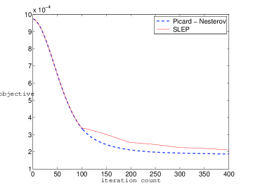
Figure 1: Objective function vs. iteration for the overlapping groups data ($d=3500$). Note that Picard-Nesterov terminates earlier within $\varepsilon$.

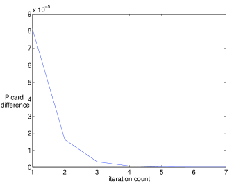
Figure 2: $\ell_{2}$ difference of successive Picard iterates vs. Picard iteration for the overlapping groups data ($d=3500$).

5.1 Overlapping Groups

In the first simulation we considered a synthetic data set which involves a fairly simple group topology which, however, cannot be embedded as a hierarchy. We generated data $A\in{\mathbb{R}}^{s\times d}$, with $s=[0.7d]$ from a uniform distribution and normalized the matrix. The target vector $x^{*}$ was also generated randomly so that only $21$ of its components are nonzero. The groups used in the regularizer ${\omega}_{GL}$ – see eq. (3.1) – are: $\{1,...,5\}$, $\{5,...,9\}$, $\{9,...,13\}$, $\{13,...,17\}$, $\{17,...,21\}$, $\{4,22,...,30\}$, $\{8,31,...,40\}$, $\{12,41,...,50\}$, $\{16,51,...,60\}$, $\{20,61,...,70\}$, $\{71,...,80\},\dots,\{d-9,...,d\}$.

That is, the first $5$ groups form a chain, the next $5$ groups have a common element with one of the first groups and the rest have no overlaps. An issue with overlapping group norms is the coefficients assigned to each group (see [12] for a discussion). We chose to use a coefficient of $1$ for every group and compensate by normalizing each component of $x^{*}$ according to the number of groups in which it appears (this of course can only be done in a synthetic setting like this). The outputs were then generated as $y=Ax^{*}+~{}\text{noise}$ with zero mean Gaussian noise of standard deviation $0.001$.

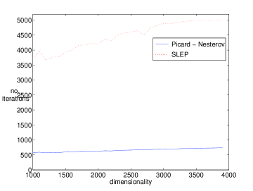
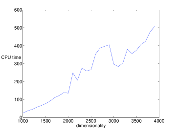
Figure 3: Average measures vs. dimensionality for the overlapping groups data. Top: number of iterations. Bottom: CPU time. Note that this time can be reduced to a fraction with a C implementation.

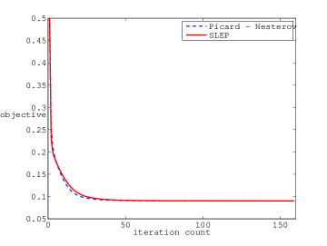
Figure 4: Objective function vs. iteration for the hierarchical overlapping groups.

We used a regularization parameter equal to $10^{-5}$. We ran the algorithm for $d=1000,1100,\dots,$ $4000$, with $10$ random data sets for each value of $d$, and compared its efficiency with SLEP. The solutions found recover the correct pattern without exact zeros due to the regularization. Figure 1 shows the number of iterations $T$ in Algorithm 2 needed for convergence in objective value within $\varepsilon=10^{-8}$. SLEP was run until the same objective value was reached. We conclude that we outperform SLEP’s $O\left(\frac{1}{T}\right)$ method. Figure 2 demonstrates the efficiency of the inner computation of the proximity map at one iteration $t$ of the algorithm. Just a few Picard iterations are required for convergence. The plots for different $t$ are indistinguishable.

Similar conclusions can be drawn from the plots in Figure 3, where average counts of iterations and CPU time are shown for each value of $d$. We see that the number of iterations depends almost linearly on dimensionality and that SLEP requires an order of magnitude more iterations – which grow at a higher rate. Note also that the cost per iteration is comparable between the two methods. We also observed that computation of the proximity map is insensitive to the size of the problem (it only requires $7-8$ iterations for all $d$). Finally, we report that CPU time grows linearly with dimensionality. To remove various overheads this estimate was obtained from Matlab’s profiling statistics for the low-level functions called. A comparison with SLEP is meaningless since the latter is a C implementation.

Besides outperforming the $O(\frac{1}{T})$ method, we also show that the Picard-Nesterov approach matches SLEP’s $O(\frac{1}{T^{2}})$ method for the tree structured Group Lasso [18]. To this end, we have imitated an experiment from [13, Sec. 4.1] using the Berkeley segmentation data set. We have extracted a random dictionary of $71$ $16\times 16$ patches from these images, which we have placed on a balanced tree with branching factors $10,2,2$ (top to bottom). Here the groups correspond to all subtrees of this tree. We have then learned the decomposition of new test patches in the dictionary basis by Group Lasso regularization (3.1). As Figure 4 shows, our method and SLEP are practically indistinguishable.

5.2 Graph Prediction

The second simulation is on the graph prediction of [11] in the limit of $p=1$ (composite $\ell_{1}$). We constructed a synthetic graph of $d$ vertices, $d=100,120,\dots,360$ with two clusters of equal size. The edges in each cluster were selected from a uniform draw with probability $\frac{1}{2}$ and we explicitly connected $d/25$ pairs of vertices between the clusters. The labeled data $y$ were the cluster labels of $s=10$ randomly drawn vertices. Note that the effective dimensionality of this problem is $O(d^{2})$. At the time of the paper’s writing there is not an accelerated method with software available online which handles a generic graph.

First, we observed that the solution found recovered perfectly the clustering. Next, we studied the decay of the objective function for different problem sizes (Figure 5). We noted a striking difference from the case of overlapping groups in that convergence now is not monotone The nature of decay also differs from graph to graph, with some cases making fast progress very close to the optimal value but long before eventual convergence. This observation suggests future modifications of the algorithm which can accelerate convergence by a factor. As an indication, the distance from the optimum was just $2.2\cdot 10^{-6},5.4\cdot 10^{-5},1.5\cdot 10^{-5}$ at iteration $611,821,418$ for $d=100,120,140$, respectively. We verified in this data as well, that Picard iterations converge very fast (Figure 6). Finally in Table 1 we report average iteration numbers and running times. These prove the feasibility of solving problems with large matrices $B$ even using a “quick and dirty” Matlab implementation.

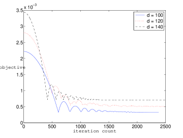
Figure 5: Objective function vs. iteration for the graph data. Note the progress in the early stages in some cases.

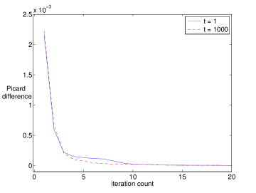
Figure 6: $\ell_{2}$ difference of successive Picard iterates vs. Picard iteration for the graph data ($d=100$).

$d$	no. iterations	CPU time (secs.)
100	2599.6	21.461
120	3680.0	54.745
140	4351.8	118.61
160	3124.8	164.21
180	2845.8	241.69
200	3476.2	359.75
220	4490.0	911.67
240	4490.0	911.67
260	3639.2	930.8

Table 1: Graph data. Note that the effective $d$ is $O(d^{2})$. CPU time can be reduced to a fraction with a C implementation.

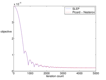
Figure 7: Objective function vs. iteration for the Fused Lasso ($d=100$). The two trajectories are identical.

In addition to a random incidence matrix, one may consider the special case of Fused Lasso or Total Variation in which $B$ has the simple form (3.2). It has been shown how to achieve the optimal $O\left(\frac{1}{T^{2}}\right)$ rate for this problem in [3]. We applied Fused Lasso (without Lasso regularization) to the same clustering data as before and compared SLEP with the Picard-Nesterov approach. As Figure 7 shows, the two trajectories are identical. This provides even more evidence in favor of optimality of our method.

6 Conclusion

We presented an efficient first order method for solving a class of nonsmooth optimization problems, whose objective function is given by the sum of a smooth term and a nonsmooth term, which is obtained by linear function composition. The prototypical example covered by this setting in a linear regression regularization method, in which the smooth term is an error term and the nonsmooth term is a regularizer which favors certain desired parameter vectors. An important feature of our approach is that it can deal with richer classes of regularizers than current approaches and at the same time is at least as computationally efficient as specific existing approaches for structured sparsity. In particular our numerical simulations demonstrate that the proposed method matches optimal $O(\frac{1}{T^{2}})$ methods on specific problems (Fused Lasso and tree structured Group Lasso) while improving over available $O(\frac{1}{T})$ methods for the overlapping Group Lasso. In addition, it can handle generic linear composite regularization problems, for many of which accelerated methods do not yet exist. In the future, we wish to study theoretically whether the rate of convergence is $O\left(\frac{1}{T^{2}}\right)$, as suggested by our numerical simulations. There is also much room for further acceleration of the method in the more challenging cases by using practical heuristics. At the same time, it will be valuable to study further applications of our method. These could include machine learning problems ranging from multi-task learning, to multiple kernel learning and to dictionary learning, all of which can be formulated as linearly composite regularization problems.

Acknowledgements

We wish to thank Luca Baldassarre and Silvia Villa for useful discussions. This work was supported by Air Force Grant AFOSR-FA9550, EPSRC Grants EP/D071542/1 and EP/H027203/1, NSF Grant ITR-0312113, Royal Society International Joint Project Grant 2012/R2, as well as by the IST Programme of the European Community, under the PASCAL Network of Excellence, IST-2002-506778.

7 Appendix

In this appendix, we collect some basic facts about fixed point theory which are useful for our study. For more information on the material presented here, we refer the reader to [37].

Let $X$ be a closed subset of ${\mathbb{R}}^{d}$. A mapping ${\varphi}:X\rightarrow X$ is called strictly non-expansive (or contractive) if there exists ${\lambda}\in[0,1)$ such that, for every $x,y\in X$,

$$\|{\varphi}(x)-{\varphi}(y)\|\leq{\lambda}\|x-y\|.$$

If the above inequality holds for $\lambda=1$, the mapping is called nonexpansive. We say that $x$ is a fixed point of ${\varphi}$ if $x={\varphi}(x)$. The Picard iterates $x^{n},n\in{\mathbb{N}}$ starting at $x_{0}\in X$ are defined by the recursive equation $x^{n}={\varphi}(x^{n-1})$.

It is a well-knwon fact that, if ${\varphi}$ is strictly nonexpansive then ${\varphi}$ has a unique fixed point $x$ and $\lim_{n\rightarrow\infty}x^{n}=x$. However, this result fails if ${\varphi}$ is nonexpansive. For example, the map ${\varphi}(x)=x+1$ does not have a fixed point. On the other hand, the identity map has infinitely many fixed points.

Definition 7.1.

Let $X$ be a closed subset of ${\mathbb{R}}^{d}$. A map ${\varphi}:X\rightarrow X$ is called asymptotically regular provided that $\lim_{n\rightarrow\infty}\|x^{n+1}-x^{n}\|=0$.

Proposition 7.1.

Let $X$ be a closed subset of ${\mathbb{R}}^{d}$ and ${\varphi}:X\rightarrow X$ such that

1. ${\varphi}$ is nonexpansive;

2. ${\varphi}$ has at least one fixed point;

3. ${\varphi}$ is asymptotically regular.

Then the sequence $\{x^{n}:n\in{\mathbb{N}}\}$ converges to a fixed point of ${\varphi}$.

Proof.

We divide the proof in three steps.

Step 1: The Picard iterates are bounded. Indeed, let $x$ be a fixed point of ${\varphi}$. We have that

$$\|x^{n+1}-x\|=\|{\varphi}(x^{n})-{\varphi}(x)\|\leq\|x^{n}-x\|\leq\cdots\leq\|x^{0}-x\|.$$

Step 2: Let $\{x^{n_{k}}:k\in{\mathbb{N}}\}$ be a convergent subsequence, whose limit we denote by $y$. We will show that $y$ is a fixed point of ${\varphi}$. Since ${\varphi}$ is continuous, we have that $\lim_{k\rightarrow\infty}(x^{n_{k}}-{\varphi}(x^{n_{k}}))=y-{\varphi}(y)$, and since ${\varphi}$ is asymptotically regular $y-{\varphi}(y)=0$.

Step 3: The whole sequence converges. Indeed, following the same reasoning in the proof of Step 1, we conclude that the sequence $\{\|x^{n}-y\|:n\in{\mathbb{N}}\}$ is non-increasing. Let $\alpha=\lim_{n\rightarrow\infty}\|x^{n}-y\|$. Since $\lim_{k\rightarrow\infty}\|x^{n_{k}}-y\|=0$, we conclude that $\alpha=0$ and, so, $\lim_{n\rightarrow\infty}x^{n}=y$. ∎

We note that in general, without the asymptotically regularity assumption, the Picard iterates do not converge. For example, consider ${\varphi}(x)=-x$. Its only fixed point is $x=0$; if we start from $x^{0}\neq 0$ the Picard iterates will oscillate. Moreover, if ${\varphi}(x)=x+1$, which is nonexpansive, the Picard iterates diverge.

We now discuss the main tool which we use to find a fixed point of a nonexpansive mapping ${\varphi}$.

Theorem 7.1.

(Opial ${{\kappa}}$-average theorem [30]) Let $X$ be a closed convex subset of ${\mathbb{R}}^{d}$, ${\varphi}:X\rightarrow X$ a nonexpansive mapping, which has at least one fixed point and let ${\varphi}_{{\kappa}}:={{\kappa}}I+(1-{{\kappa}}){\varphi}$. Then, for every ${{\kappa}}\in(0,1)$, the Picard iterates of ${\varphi}_{{\kappa}}$ converge to a fixed point of ${\varphi}$.

We prepare for the proof with two useful lemmas.

Lemma 7.1.

If ${{\kappa}}\in(0,1)$, $u,w\in{\mathbb{R}}^{d}$, $\|u\|\leq\|w\|$, then

$$\kappa(1-\kappa)\|w-u\|^{2}\leq\|w\|^{2}-\|{{\kappa}}w+(1-{{\kappa}})u\|^{2}$$

Proof.

The assertion follows from $\ell_{2}$ strong convexity,

$$\kappa(1-\kappa)\|w-u\|^{2}+\|{{\kappa}}w+(1-{{\kappa}})u\|^{2}$$

$$={{\kappa}}\|w\|^{2}+(1-{{\kappa}})\|u\|^{2}\leq\|w\|^{2}\,.$$

∎

Lemma 7.2.

If $\{u^{n}:n\in{\mathbb{N}}\}$ and $\{w^{n}:n\in{\mathbb{N}}\}$ are sequences in ${\mathbb{R}}^{d}$ such that $\lim_{n\rightarrow\infty}\|w^{n}\|=1$, $\|u^{n}\|\leq\|w^{n}\|$ and $\lim_{n\rightarrow\infty}\|{{\kappa}}w^{n}+(1-{{\kappa}})u^{n}\|=1$, then $\lim_{n\rightarrow\infty}w^{n}-u^{n}=0$.

Proof.

Apply Lemma 7.1 to note that

$${{\kappa}}(1-{{\kappa}})\|w^{n}-u^{n}\|^{2}\leq\|w^{n}\|^{2}-\|{{\kappa}}w^{n}+(1-{{\kappa}})u^{n}\|^{2}.$$

By hypothesis the right hand side tends to zero as $n$ tends to infinity and the result follows. ∎

Proof of Theorem 7.1.

Let $\{x^{n}:n\in{\mathbb{N}}\}$ be the iterates of ${\varphi}_{{\kappa}}$. We will show that ${\varphi}_{{\kappa}}$ is asymptotically regular. The result will then follow by Proposition 7.1 and the fact that ${\varphi}_{{\kappa}}$ and ${\varphi}$ have the same set of fixed points.

Let $x^{n+1}={{\kappa}}x^{n}+(1-{{\kappa}}){\varphi}(x^{n})$. Note that, if $u$ is fixed point of ${\varphi}_{{\kappa}}$, then

$$\|x^{n+1}-u\|\leq\|x^{n}-u\|\leq\cdots\leq\|x^{0}-u\|\,.$$

Let $\overline{d}:=\lim_{n\rightarrow\infty}\|x^{n}-u\|$. If $\overline{d}=0$ the result is proved. We will show that if $\overline{d}>0$ we contradict the hypotheses of the theorem. For every $n\in{\mathbb{N}}$, we define $w^{n}=\overline{d}^{-1}(x^{n}-u)$ and $u^{n}=\overline{d}^{-1}({\varphi}(x^{n})-u)$. Note that the sequences $\{w^{n}:n\in{\mathbb{N}}\}$ and $\{u^{n}:n\in{\mathbb{N}}\}$ satisfy the hypotheses of Lemma 7.2. Thus, we have that $\lim_{n\rightarrow\infty}(x^{n}-{\varphi}(x^{n}))=0$. Consequently $x^{n+1}-x^{n}=(1-{{\kappa}})({\varphi}(x^{n})-x^{n})\rightarrow 0$, showing that $\{x^{n}:n\in{\mathbb{N}}\}$ is asymptotically regular. ∎

References

- [1] A. Argyriou, T. Evgeniou, and M. Pontil. Convex multi-task feature learning. Machine Learning, 73(3):243–272, 2008.
- [2] A. Argyriou, C.A. Micchelli, and M. Pontil. On spectral learning. The Journal of Machine Learning Research, 11:935–953, 2010.
- [3] A. Beck and M. Teboulle. Fast gradient-based algorithms for constrained total variation image denoising and deblurring problems. Image Processing, IEEE Transactions on, 18(11):2419–2434, 2009.
- [4] A. Beck and M. Teboulle. A fast iterative shrinkage-thresholding algorithm for linear inverse problems. SIAM Journal of Imaging Sciences, 2(1):183–202, 2009.
- [5] S. Becker, E. J. Candès, and M. Grant. Templates for convex cone problems with applications to sparse signal recovery. Preprint, 2010.
- [6] J. M. Borwein and A. S. Lewis. Convex Analysis and Nonlinear Optimization: Theory and Examples. CMS Books in Mathematics. Springer, 2005.
- [7] P.L. Combettes and V.R. Wajs. Signal recovery by proximal forward-backward splitting. Multiscale Modeling and Simulation, 4(4):1168–1200, 2006.
- [8] I. Daubechies, R. DeVore, M. Fornasier, and C.S. Güntürk. Iteratively reweighted least squares minimization for sparse recovery. Communications on Pure and Applied Mathematics, 63(1):1–38, 2010.
- [9] J. Duchi and Y. Singer. Efficient online and batch learning using forward backward splitting. The Journal of Machine Learning Research, 10:2899–2934, 2009.
- [10] T. Evgeniou, M. Pontil, and O. Toubia. A convex optimization approach to modeling consumer heterogeneity in conjoint estimation. Forthcoming at Marketing Science, 2007.
- [11] M. Herbster and G. Lever. Predicting the labelling of a graph via minimum p-seminorm interpolation. In Proceedings of the 22nd Conference on Learning Theory (COLT), 2009.
- [12] R. Jenatton, J.-Y. Audibert, and F. Bach. Structured variable selection with sparsity-inducing norms. arXiv:0904.3523v2, 2009.
- [13] R. Jenatton, J. Mairal, G. Obozinski, and F. Bach. Proximal methods for sparse hierarchical dictionary learning. In International Conference on Machine Learning, pages 487–494, 2010.
- [14] D. Kim, S. Sra, and I. S. Dhillon. A scalable trust-region algorithm with application to mixed-norm regression. In International Conference on Machine Learning, 2010.
- [15] Q. Lin. A Smoothing Stochastic Gradient Method for Composite Optimization. Arxiv preprint arXiv:1008.5204, 2010.
- [16] J. Liu, S. Ji, and J. Ye. SLEP: Sparse Learning with Efficient Projections. Arizona State University, 2009.
- [17] J. Liu and J. Ye. Fast Overlapping Group Lasso. Arxiv preprint arXiv:1009.0306, 2010.
- [18] J. Liu and J. Ye. Moreau-Yosida regularization for grouped tree structure learning. In Advances in Neural Information Processing Systems, 2010.
- [19] J. Liu, L. Yuan, and J. Ye. An efficient algorithm for a class of fused lasso problems. In Proceedings of the 16th ACM SIGKDD international conference on Knowledge discovery and data mining, pages 323–332, 2010.
- [20] J. Mairal, R. Jenatton, G. Obozinski, and F. Bach. Network flow algorithms for structured sparsity. CoRR, abs/1008.5209, 2010.
- [21] C.A. Micchelli, L. Shen, and Y. Xu. Proximity algorithms for image models: denoising. preprint, September 2010.
- [22] J.J. Moreau. Fonctions convexes duales et points proximaus dans un espace hilbertien. Acad. Sci. Paris Sér. A Math., 255:2897–2899, 1962.
- [23] J.J. Moreau. Proximité et dualité dans un espace hilbertien. Bull. Soc. Math. France, 93(2):273–299, 1965.
- [24] S. Mosci, L. Rosasco, M. Santoro, A. Verri, and S. Villa. Solving Structured Sparsity Regularization with Proximal Methods. In Proc. European Conf. Machine Learning and Knowledge Discovery in Databases, pages 418–433, 2010.
- [25] A. S. Nemirovsky and D. B. Yudin. Problem complexity and method efficiency in optimization. Wiley, 1983.
- [26] Y. Nesterov. A method of solving a convex programming problem with convergence rate . Soviet Mathematics Doklady, 27(2):372–376, 1983.
- [27] Y. Nesterov. Smooth minimization of non-smooth functions. Mathematical Programming, 103(1):127–152, 2005.
- [28] Y. Nesterov. Gradient methods for minimizing composite objective function. CORE, 2007.
- [29] Y. Nesterov and A. Nemirovskii. Interior-point polynomial algorithms in convex programming. Number 13. Society for Industrial Mathematics, 1987.
- [30] Z. Opial. Weak convergence of the subsequence of successive approximations for nonexpansive operators. Bulletin American Mathematical Society, 73:591–597, 1967.
- [31] M.R. Osborne. Finite algorithms in optimization and data analysis. John Wiley & Sons, Inc. New York, NY, USA, 1985.
- [32] R. Tibshirani, M. Saunders, S. Rosset, J. Zhu, and K. Knight. Sparsity and smoothness via the fused lasso. Journal of the Royal Statistical Society: Series B (Statistical Methodology), 67(1):91–108, 2005.
- [33] P. Tseng. On accelerated proximal gradient methods for convex-concave optimization. Preprint, 2008.
- [34] P. Tseng. Approximation accuracy, gradient methods, and error bound for structured convex optimization. Mathematical Programming, 125(2):263–295, 2010.
- [35] J. Von Neumann. Some matrix-inequalities and metrization of matric-space. Mitt. Forsch.-Inst. Math. Mech. Univ. Tomsk, 1:286–299, 1937.
- [36] M. Yuan and Y. Lin. Model selection and estimation in regression with grouped variables. Journal of the Royal Statistical Society, Series B, 68(1):49–67, 2006.
- [37] C. Zlinescu. Convex Analysis in General Vector Spaces. World Scientific, 2002.
- [38] P. Zhao, G. Rocha, and B. Yu. Grouped and hierarchical model selection through composite absolute penalties. Annals of Statistics, 37(6A):3468–3497, 2009.