Itinerant ferromagnetism in an interacting Fermi gas with mass imbalance

Abstract

We study the emergence of itinerant ferromagnetism in an ultra-cold atomic gas with a variable mass ratio between the up and down spin species. Mass imbalance breaks the SU(2) spin symmetry leading to a modified Stoner criterion. We first elucidate the phase behavior in both the grand canonical and canonical ensembles. Secondly, we apply the formalism to a harmonic trap to demonstrate how a mass imbalance delivers unique experimental signatures of ferromagnetism. These could help future experiments to better identify the putative ferromagnetic state. Furthermore, we highlight how a mass imbalance suppresses the three-body loss processes that handicap the formation of a ferromagnetic state. Finally, we study the time dependent formation of the ferromagnetic phase following a quench in the interaction strength.

I Introduction

By exploiting the fine control of interactions through a magnetically tuned Feshbach resonance 76s12 , ultracold atomic Fermi gases have proven to be a rich arena in which to study many-body physics. On one side of the Feshbach resonance the effective s-wave interaction is attractive, which has allowed investigators to realize a BCS state of Cooper pairs. If the interactions are tuned across the Feshbach resonance, the fermions bind to form molecules that can subsequently form a Bose-Einstein condensate 03sph08 . However, the fermions experience repulsive interactions if the Feshbach resonance is approached from the other side. A recent experiment by the MIT group Jo09 on the repulsive side of the resonance has provided the first tentative evidence for the formation of an itinerant ferromagnetic phase. There was however a significant atom loss process that could drive the formation of alternative strongly correlated states Pekker10 , which are consistent with some of the experimental results. It is therefore essential to develop a different realization of the ferromagnetic state which suppresses atom loss, and in addition delivers unique experimental signatures to help resolve the outstanding questions over the original experiment. If the experiment were confirmed Houbiers97 ; Duine05 ; LeBlanc09 ; Conduit10 , the flexibility offered by ultracold atomic gases now presents investigators with a unique opportunity to study aspects of ferromagnetism that cannot be envisioned in the solid state, including the consequences of population imbalance Conduit08 , a conserved net magnetization Berdnikov09 , the damping of quantum fluctuations by three-body loss Conduit10ii , single spin flips Zhai09 , spin drag Duine10 , spin spiral formation Conduit-Altman , reduced dimensionality Conduit-2D , as well as ferromagnetic phenomena in an optical lattice FerroLattice . In this paper we turn to consider the consequences of the up and down-spin particles carrying different masses, a scenario that cannot be realized in the solid state. Furthermore the system offers investigators a lower atom loss rate combined with inimitable experimental signatures.

The MIT experiment prepared an ultracold atomic gas with two different atomic species to represent the pseudo up and down spin fermions. In the experiment, and all theoretical studies of itinerant ferromagnetism to date, the two species are different electronic states of the same atom, and therefore carry the same mass. This accurately reflects the situation in solid state ferromagnetism where the up and down-spin electrons have the same effective mass. However, the flexibility introduced by the new experimental realization of ferromagnetism permits the pseudo up and down spins to be represented by two species of atoms of different elements with unequal masses; alternatively an optical lattice can change the effective mass of the atoms. Though in the solid state interactions can change the effective mass of the majority and minority spin species Hirsch00 , distinct species of fermions in an ultracold atomic gas provide a cleaner and more controlled realization of mass imbalance. Furthermore, introducing a mass ratio breaks the SU(2) symmetry of the conventional ferromagnet, and as a result the magnetization has anisotropic susceptibility and so offers a novel control parameter over magnetic ordering and unique experimental signatures of the ferromagnetic state. Moreover, introducing a mass imbalance should suppress the three-body losses that hinder ultracold atom experiments Petrov03 . Further motivation to study a generalized mass ratio stems from novel physics discovered on the attractive side of the Feshbach resonance. It has been established that imbalanced Fermi surfaces in a superfluid can drive the formation of the textured Fulde-Ferrel-Larkin-Ovchinnikov phase FFLOPapers , and here we explore the opportunity that new phenomena could arise in a mass imbalanced itinerant ferromagnet.

In this paper in Sec. II we first develop the formalism required to study a mass imbalanced Fermi gas with repulsive interactions. Subsequently in Sec. III we derive the general phase diagram for a uniform gas with both a generalized mass ratio and also population imbalance. To cement the connection to the recent possible experimental observation of ferromagnetism in an ultracold atom gas, we consider the consequences of a trapped geometry and study the quantities observable by experiments in Sec. IV. In the current experimental realization of ferromagnetism there were significant three-body losses so the ferromagnetic phase was formed following a quench in the interaction strength out of equilibrium. Therefore in Sec. V we conclude our investigation by studying the dynamical formation of the ferromagnetic phase. Finally, we summarize our discussion of itinerant ferromagnetism in Sec. VI.

II Formalism

To study itinerant ferromagnetism in the presence of a mass imbalance we use the functional integral formalism developed in Ref. Conduit08 . The phase diagram predicted there has recently been verified by ab initio quantum Monte Carlo studies Conduit09 ; Pilati10 and is also in accord with recent experimental findings Jo09 ; LeBlanc09 ; Conduit10 . Therefore, the approach described in Ref. Conduit08 provides a solid platform from which to investigate itinerant ferromagnetism with a mass imbalance.

The formalism centers around calculating the quantum partition function expressed as a coherent state field integral

$$\mathcal{Z}\!=\!\!\int\!\!\mathcal{D}\psi\text{exp}\Bigg{[}\!-\!\!\int\!\!\!\!\!\sum_{\sigma=\left\{\uparrow,\downarrow\right\}}\!\!\!\!\overline{\psi}_{\sigma}(\!\hat{\partial}_{\tau}\!+\!\hat{\xi}_{\sigma}\!)\psi_{\sigma}\!-\!g\!\int\!\overline{\psi}_{\uparrow}\overline{\psi}_{\downarrow}\psi_{\downarrow}\psi_{\uparrow}\Bigg{]}\,.$$ (1)

Here the field $\psi$ describes a two component Fermi gas with a repulsive s-wave contact interaction $g\delta^{3}(\mathbf{r})$ acting between the two species. We use the notation $\int\equiv\int_{0}^{\beta}\text{d}\tau\int\text{d}\mathbf{r}$ with inverse temperature $\beta=1/k_{\text{B}}T$, and dispersion $\hat{\xi}_{\sigma}=\hat{p}^{2}/2m_{\sigma}-\mu_{\sigma}$. It will later be convenient to rewrite the particle masses as $m_{\sigma}=m(1+\sigma r)$, and the species chemical potentials as $\mu_{\sigma}=\mu+\sigma\Delta\mu$. Here $\sigma\in\{\uparrow,\downarrow\}$ is a label to distinguish between the two species of atoms and does not represent a physical spin.

We now decouple the quartic interaction term, which will allow us to integrate out the fermionic degrees of freedom. Hertz did this by introducing a scalar Hubbard-Stratonovich decoupling of the two-body interaction term into the magnetization channel Hertz . By expanding in the magnetization he was able to develop an effective Landau theory. However, recent studies have shown that this approach fails to recover the correct Hartree-Fock equations, and capture the behavior of the soft transverse degrees of freedom Conduit08 . Moreover, as mass imbalance breaks the SU(2) symmetry of the system, magnetization formed along the quantization axis is distinctly different from perpendicular magnetization. We therefore adapt the formalism developed in Ref. Conduit08 , and decouple the quartic interaction term in the full vector magnetization $\boldsymbol{\phi}$ as well as the density channel $\rho$. This yields an action that is quadratic in the fermion degrees of freedom, and after integrating them out we recover the quantum partition function $\mathcal{Z}=\int\mathcal{D}\boldsymbol{\phi}\mathcal{D}\rho\exp(-S)$ with an action

$$S\!=\!\int\!g(\boldsymbol{\phi}^{2}\!-\!\rho^{2})\!-\!\operatorname{Tr}\ln\left[(\hat{\partial}_{\tau}\!+\!\hat{\xi}_{\alpha}\!+\!g\rho)\mathbf{I}-g\boldsymbol{\phi}\cdot\boldsymbol{\sigma}\right]\,.$$ (2)

We now focus on the saddle point fields (or “mean-fields”) of the action, that is $\boldsymbol{\phi}$ and $\rho$ satisfying $\delta S/\delta\boldsymbol{\phi}=0$ and $\delta S/\delta\rho=0$. We show in Sec. V.1 that fluctuations are gapped so we neglect the fluctuation corrections and assume that the saddle point fields make the dominant contribution to the partition function. We then diagonalize the inverse Green function inside the trace to the new basis set $\chi\in\{+,-\}$, and perform the summation over Matsubara frequencies. Finally we use $\Phi=-k_{\text{B}}T\ln(\mathcal{Z})$ to yield the thermodynamic grand potential

$$\Phi\!=\!gV(\boldsymbol{\phi}^{2}\!-\!\rho^{2})\!-\!k_{\text{B}}T\!\!\!\!\!\sum_{\chi\in\{+,-\}}\int\!\text{d}\epsilon\,\nu(\epsilon)\ln\left(1\!+\!\text{e}^{-\beta\zeta_{\chi}}\right)\,,$$ (3)

where $V$ is the total volume, $\nu(\epsilon)=m^{3/2}\sqrt{\epsilon}/\pi^{2}\hbar^{3}\sqrt{2}$ is the density of states, and effective dispersion

$$\zeta_{\pm}\!=\!\frac{\epsilon}{1-r^{2}}\!-\!\mu\!+\!g\rho\pm\sqrt{(g\phi_{\perp})^{2}\!+\!\left(\frac{\epsilon r}{1-r^{2}}\!+\!\Delta\mu\!+\!g\phi_{\text{z}}\right)^{2}}\,.$$ (4)

Varying the grand potential $\Phi$ with respect to $\boldsymbol{\phi}$ and $\rho$ yields the saddle point equations for the homogeneous mean-fields. We have checked numerically in Sec. III and analytically in Sec. V.1 that any gas with a mass and/or chemical potential imbalance breaks the SU(2) symmetry and does not develop perpendicular magnetization, so $\phi_{\perp}=0$. This result considerably simplifies the mean-field equations. As the particle densities are related to the saddle point fields through $n_{\sigma}=\rho+\sigma\phi_{\text{z}}$, at zero temperature we cast the mean-field equations as

$$n_{\sigma}=\frac{\sqrt{2}}{3\pi^{2}\hbar^{3}}m_{\sigma}^{3/2}\left(\mu_{\sigma}-gn_{-\sigma}\right)^{3/2}\,,$$ (5)

which shows that the Fermi energy of the $\sigma$ species is $\epsilon_{\text{F}\sigma}=\mu_{\sigma}-gn_{-\sigma}$. This equation forms the backbone of our subsequent analysis. We first use it to derive a generalized Stoner criterion for the ferromagnetic instability in a mass imbalanced gas. Such a transition is characterized by the appearance of three nearby solutions; the now unstable original state, and two with small relative positive and negative polarization. Demanding the existence of these solutions to the self-consistent equations (5) yields a modified Stoner criterion $g\sqrt{\nu_{\uparrow}\nu_{\downarrow}}=1$, where the $\nu_{\sigma}$ is a density of states at the $\sigma$ species Fermi surface. This reduces to the familiar criterion $g\nu=1$ in the mass and population balanced limit Stoner .

In Sec. V.2 we show that the saddle point fields are always uniform, even for general chemical potential and mass imbalance. Therefore, unlike the superfluid regime where a Fermi surface imbalance can drive the formation of the textured Fulde-Ferrel-Larkin-Ovchinnikov state FFLOPapers , here for a perfectly spherical Fermi surface and the absence of nesting only uniform ferromagnetic states will be formed. We note however that fluctuation corrections drive textured phase formation in the equal mass case Conduit09 , and have the potential to do the same with mass imbalance.

III Phase Diagram

Now that we have prepared the formalism we are ideally placed to study the phase diagram of the mass imbalanced Fermi gas with repulsive interactions. This will allow us to build up an intuition for the consequences of mass imbalance before we turn to study the gas in a harmonic trap in Sec. IV. Firstly, in Sec. III.1, we examine the grand canonical ensemble with a gas connected to an infinite particle reservoir, and secondly in Sec. III.2 we study the gas with a constant number of particles in the canonical ensemble. To cement the connection to experiment, from now on we express the interaction strength as $k_{\text{F}}a$, the product of the Fermi wave vector $k_{\text{F}}$ of a non-interacting gas with the same net number density, and the scattering length $a=g/2\pi\hbar^{2}(1/m_{\uparrow}+1/m_{\downarrow})+\mathcal{O}(g^{2})$ Meystre01 . Consistent with the Hartree-Fock scheme we employed to calculate the grand thermodynamic potential Eq. (3) we have taken the lowest order term in the scattering length and neglected higher order corrections in $g$ Duine05 ; Conduit08 ; Zhou11 . We concentrate on the phase behavior at $T=0$.

III.1 Grand canonical ensemble

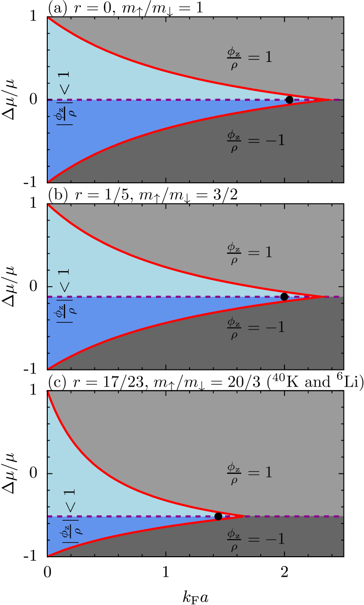
Figure 1: (Color online) The phase behavior in the grand canonical ensemble with chemical potential imbalance $\Delta\mu/\mu$ and interaction strength $k_{\text{F}}a$ for three different values of mass imbalance. The solid red lines denote the onset of full polarization, into the phases shaded light and dark gray for up ($\phi_{\text{z}}/\rho=1$) and down ($\phi_{\text{z}}/\rho=-1$) spin respectively. The dashed purple boundary separates systems that become polarized in the up (above dashed line, light blue shading) or down-spin (below dashed line, dark blue shading) directions in the strongly interacting limit. Along the dashed purple line itself the polarization remains constant until reaching the black dot, past which polarization in either direction is equally favorable.

In the grand canonical ensemble the gas can exchange particles with an ideal reservoir. We can control the average number density of atoms by manipulating the chemical potentials $\mu_{\sigma}$ of the reservoir.

To develop a physical understanding and connect with previous work LeBlanc09 ; Conduit08 ; Conduit10 we first describe the phase diagram for a gas without a mass imbalance shown in Fig. 1(a). When the gas is noninteracting it is paramagnetic for all chemical potential imbalances $\Delta\mu=\mu_{\uparrow}-\mu_{\downarrow}$. Above the line $\Delta\mu=0$, increasing the interaction strength drives polarization in the up-spin direction. Conversely, below $\Delta\mu=0$ the gas becomes polarized in the down-spin direction. As the interaction strength is increased across the boundary marked on Fig. 1(a) the gas enters the fully polarized state. For more positive $\Delta\mu$, the gas becomes fully polarized in the $\uparrow$ direction at lower interaction strength. We can understand the form of the boundary line at $\Delta\mu>0$ by examining the species Fermi energies $\epsilon_{\text{F}\sigma}=\mu+\sigma\Delta\mu-gn_{-\sigma}$. At $g=0$ the Fermi energies are simply the chemical potentials, so $n_{\uparrow}>n_{\downarrow}$. The result is that $\epsilon_{\text{F}\downarrow}$ is smaller than $\epsilon_{\text{F}\uparrow}$ at zero interaction, and decreases more rapidly with increasing interaction strength. Thus the gas becomes fully polarized more quickly in the $\uparrow$ direction as we increase the chemical potential bias. An analogous situation occurs in the bottom half of Fig. 1(a), where $\uparrow$ and $\downarrow$ swap roles in the argument above. The line separating these two regimes is $\Delta\mu=0$. As the interaction strength is increased along this line the magnetization remains pinned at zero until $k_{\text{F}}a\approx 2.04$, at which point a ferromagnetic instability develops and the gas can become polarized in any direction. The instability to full polarization at $k_{\text{F}}a=3\pi/4$ coincides with the cusped junction of the fully polarized region boundary.

When we introduce a mass imbalance, for any chemical potential and interaction strength, the saddle point solutions have $\phi_{\perp}=0$. The phase behavior shown in Fig. 1(b and c) is then obtained using the zero temperature mean-field equations (5). At zero interaction strength when there is no chemical potential imbalance, the number density of the species is $n_{\sigma}=(\sqrt{2}/3\pi^{2}\hbar^{3})m_{\sigma}^{3/2}\mu^{3/2}$, and so an increase in the mass imbalance alone will bias the system towards the heavy spin species. Then, as we increase the interaction strength, the Fermi energy $\epsilon_{\text{F}\downarrow}=\mu-gn_{\uparrow}$ of the minority lighter species will fall more rapidly than that of the heavy species $\epsilon_{\text{F}\uparrow}=\mu-gn_{\downarrow}$, and so the gas becomes fully polarized towards the heavier species. With the heavier species becoming favored, the border in Fig. 1(b and c) between the dominant heavy and light spin polarization shifts downwards towards the lighter spin particles. In order to have neither species dominant at full polarization, we need to introduce a chemical potential imbalance that favors the lighter species, given by the implicit equation

$$\frac{\Delta\mu}{\mu}\!=\!\frac{[(1\!-\!r)(\mu\!-\!\Delta\mu)]^{3/2}\!-\![(1\!+\!r)(\mu\!+\!\Delta\mu)]^{3/2}}{[(1\!-\!r)(\mu\!-\!\Delta\mu)]^{3/2}\!+\![(1\!+\!r)(\mu\!+\!\Delta\mu)]^{3/2}}\,.$$ (6)

If the chemical potentials are tuned according to Eq. (6), then at low interaction strength the magnetization is pinned to $-\Delta\mu/\mu$. Increasing the interaction strength past a critical value (denoted by the black dot in Fig. 1) induces a second order phase transition in the magnetization; the minimum in the grand potential at $-\Delta\mu/\mu$ bifurcates into two equally favorable minima which move continuously to full up and down polarization as we further increase the interaction strength. Full polarization emerges at an interaction strength

$$k_{\text{F}}a=\frac{3\pi\hbar k_{\text{F}}}{2\sqrt{2}\left(1/m_{\uparrow}+1/m_{\downarrow}\right)}\max_{\sigma}\left(\frac{\mu_{-\sigma}}{(m_{\sigma}\mu_{\sigma})^{3/2}}\right)\,.$$ (7)

Having understood the behavior of the gas in the grand canonical ensemble we now disconnect the particle reservoirs and study a gas in the canonical ensemble.

III.2 Canonical ensemble

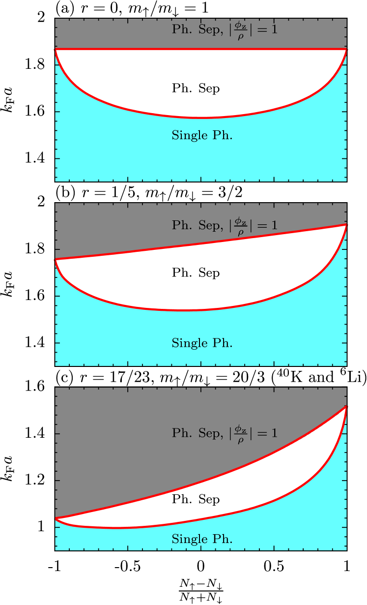
Figure 2: (Color online) The phase behavior in the canonical ensemble with interaction strength $k_{\text{F}}a$ and net population imbalance $(N_{\uparrow}-N_{\downarrow})/(N_{\uparrow}+N_{\downarrow})$ for three different values of mass imbalance $r$. The light blue regions (Single Ph.) correspond to a paramagnetic gas, white (Ph. Sep) to a two-phase coexistence between two partially polarized gases, and dark gray (Ph. Sep, $|\frac{\phi_{\text{z}}}{\rho}|=1$) to a two-phase coexistence between two fully polarized up and down spin gases.

We now investigate a gas confined so that the total number of both species is held fixed. In a cold atom gas the number of up and down particles are separately conserved, and so at the ferromagnetic transition the gas splits into up and down polarized domains. On increasing the interaction strength the gas could potentially phase separate into majority up and majority down-spin domains to reduce contact between the two species. The formation of this ferromagnetic state is governed by the competition between the resulting fall in interaction energy and a kinetic energy penalty due to the increased density of each separate species.

A box of gas with fixed total particle numbers is described by minimizing the total free energy. The free energy density of a single domain with particle densities $n_{\uparrow}$ and $n_{\downarrow}$ is obtained from the grand potential Eq. (3) by substituting our mean-field solutions Eq. (5) into the definition $F=\Phi+\mu_{\uparrow}n_{\uparrow}V+\mu_{\downarrow}n_{\downarrow}V$, which yields

$$\frac{F}{V}=\frac{3}{5}\left(\frac{3\pi^{2}\hbar^{3}}{\sqrt{2}}\right)^{2/3}\left[\frac{n_{\uparrow}^{5/3}}{m_{\uparrow}}+\frac{n_{\downarrow}^{5/3}}{m_{\downarrow}}\right]+gn_{\uparrow}n_{\downarrow}\,.$$ (8)

If there is no phase separation, the total free energy of the gas is just that of a single domain. This state competes with a phase separated gas containing two domains, labeled A and B, with a ratio of volumes $\gamma$, and particle densities $n_{\text{A}\sigma}$ and $n_{\text{B}\sigma}$. The total energy of the state is then $F=\gamma F_{\text{A}}+(1-\gamma)F_{\text{B}}$, and the total particle numbers are $N_{\sigma}=V\left(\gamma n_{\text{A}\sigma}+\left(1-\gamma\right)n_{\text{B}\sigma}\right)$. We then minimize the total free energy while fixing the $N_{\sigma}$, to determine whether the system phase separates, and if so the properties of the individual domains. The resulting phase diagrams are shown in Fig. 2.

To explore the phase behavior in the canonical ensemble, and to establish a connection to the literature Conduit08 , we first focus on the mass balanced case shown in Fig.2(a). At weak interactions the gas starts in the paramagnetic state. On ramping the interaction strength through the Stoner criterion at $k_{\text{F}}a=\pi/2$, a system with zero net population imbalance phase separates into two weakly but oppositely polarized domains. The critical interaction strength for phase separation is higher in the presence of a population imbalance due to the larger kinetic energy barrier that must be overcome for further polarization to form. A fully polarized phase forms at $k_{\text{F}}a=3\pi/2^{7/3}$, which is in accordance with Ref. Conduit08 ; LeBlanc09 .

On introducing a mass imbalance the phase diagrams tilt so that when the population imbalance is towards the lighter species, the onset of full phase separation takes place at smaller $k_{\text{F}}a$. To understand this, we first derive an expression for the interaction strength at which the system becomes fully polarized. At this point, there is an A phase composed entirely of the heavier $\uparrow$ particles and a B phase of the lighter $\downarrow$ particles. Just before the transition to full polarization, there will still be a $\downarrow$ particle in the A phase. This has interaction energy $g_{\text{fp}}n_{\uparrow}$. If that atom transits into phase B it sits on top of the Fermi surface, with an energy penalty $Dn_{\downarrow}^{2/3}/m_{\downarrow}$, where $D=3^{5/3}\pi^{4/3}\hbar^{2}/2^{1/3}5$. At the transition to full polarization the particle makes this passage without hindrance, and therefore these two energies are equal $g_{\text{fp}}n_{\uparrow}=Dn_{\downarrow}^{2/3}/m_{\downarrow}$. This implies that the interaction strength at the phase transition is $g_{\text{fp}}=Dn_{\downarrow}^{2/3}/m_{\downarrow}n_{\uparrow}=Dn_{\uparrow}^{2/3}/m_{\uparrow}n_{\downarrow}$; to deduce the second equality we have repeated the argument for down spin particles. The second equality implies that $n_{\downarrow}^{5/3}/m_{\downarrow}=n_{\uparrow}^{5/3}/m_{\uparrow}$, which confirms that the two regions have equal pressure.

We now use the above expressions to explain the tilt in the fully polarized phase boundary Fig. 2(b) and (c). To go from population balance to a system imbalanced towards the light particles, we imagine converting a region of heavy particles into light. However, for a given density, the lighter particles exert a greater degeneracy pressure $P\propto n^{5/3}/m$ than heavier particles and so the internal pressure within the system must increase. This compresses both the light and heavy particle domains, and since $n_{\downarrow}^{5/3}/m_{\downarrow}=n_{\uparrow}^{5/3}/m_{\uparrow}$ the overall density of both phases must increase by the same ratio. Therefore, upon biasing the population towards the lighter species the critical interaction strength $g_{\text{fp}}\propto n_{\downarrow}^{2/3}/n_{\uparrow}$ must decrease, thus tilting the phase boundary.

IV Trapped geometry & experimental observation

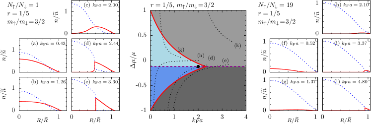
Figure 3: (Color online) Trap-profiles for a gas at various interaction strengths with a mass imbalance $m_{\uparrow}/m_{\downarrow}=3/2$. Figures (a to e) for a cloud with $N_{\uparrow}/N_{\downarrow}=1$ show the density of the heavier particles (dotted) and the density of lighter particles (solid) against radius. The axes are normalized by $\widetilde{n}$, the density of the heavier particles at the center of the trap when $k_{\text{F}}a=0$, and $\widetilde{R}$, the cloud size when $k_{\text{F}}a=0$. Figures (f to j) show the density profiles for a cloud with $(N_{\uparrow}-N_{\downarrow})/(N_{\uparrow}+N_{\downarrow})=0.9$. At the center a grand canonical phase diagram reproduced from Fig. 1 shows dotted trajectories in parameter space corresponding to some of the trap-profiles and (k) is referenced in the text.

Having understood the behavior in the canonical and grand canonical ensembles in a uniform background potential, we are well positioned to study the experimental realization of the gas in a harmonic trap potential $V(R)=\omega R^{2}$. We employ the local-density approximation and so assume that the properties of the gas at radius $R$ are determined by substituting a local chemical potential $\mu_{\sigma}(R)=\mu_{\sigma}-V(R)$ into our mean-field relations Eq. (5). Moving outwards from the center of the trap, the system parameters trace trajectories on the grand canonical phase diagrams Fig. 1. An immediate corollary is that the gas becomes polarized only along the quantization axis, and so the gas separates into domains of light and heavy particles. The chemical potentials $\mu_{\sigma}$ at the center of the trap are chosen to ensure that the cloud contains a fixed total number of atoms, and then the properties of the gas are entirely determined by the interaction strength and particle masses. In what follows, we will be interested in four main trap observables: the number density profiles of the two species, the total trap-size, and loss rate, which can all be measured by imaging the spatial distribution of the atoms in situ, and the total kinetic energy, measured by tracking the profile of the atoms following a ballistic expansion. Following Petrov03 , we model the loss rate density according to $\Upsilon n_{\uparrow}n_{\downarrow}a^{6}$, where $\Upsilon$ contains the residual mass and number density terms. $\Upsilon$ has a non-monotonic mass ratio dependence Petrov03 , leading to a dramatic suppression of loss rate for moderately large mass imbalances (for example a gas containing ⁴⁰K and ⁶Li has $m_{\uparrow}/m_{\downarrow}=20/3$, which we show reduces loss by at least a factor of 20).

We are interested in how mass imbalance affects these four experimental observables, but to contrast our results with earlier work, we first review the mass balanced case. After that, we introduce mass imbalance and expose unique signatures of the ferromagnetic phase.

IV.1 Mass balanced gas

We start by examining a trap with a two component Fermi gas with mass balance, but variable population imbalance. To understand the corresponding trends in Fig. 4 (comparing solid red curves in the same row), it is first useful to note how the species are redistributed in the trap as we increase the repulsive interaction strength.

Density profiles: At zero interaction, both species have identical smooth distributions in the trap. Upon increasing $k_{\text{F}}a$, the species spread themselves more thinly across the trap to reduce repulsion. As the interaction strength passes a critical threshold, magnetic domains are formed in the center of the trap via a spontaneous symmetry breaking Babadi09 . However, because the density (and hence effective interaction strength) decreases at larger radii, the gas remains paramagnetic there. The width of this outer paramagnetic region falls as $\sim 1/(k_{\text{F}}a)^{2}$ in the large $k_{\text{F}}a$ limit. On introducing a population imbalance, some of the minority spin particles are driven to larger radii with increasing $k_{\text{F}}a$. This is because the minority species feels an interaction energy proportional to the density of the majority species, which overcomes the trapping potential. For large enough $k_{\text{F}}a$, domains form in the central regions of the trap. These become fully polarized as the interaction strength continues to increase. In this fully polarized limit there is no overlap between the species so the interaction energy disappears and both species can be found in domains anywhere across the trap.

Cloud size: In the non-interacting limit, a cloud with a population imbalance contains more of the majority spin species so has a greater initial radius. Initially, cloud size increases linearly at small $k_{\text{F}}a$ as the atoms repel and spread themselves more sparsely through the trap. After the atoms enter ferromagnetic domains, firstly at the center and later across the entire trap, the cloud size asymptotes towards its large $k_{\text{F}}a$ limit. At strong interactions the fully polarized domains contain effectively a non-interacting gas and so the cloud size is the same as for the population balanced case.

Kinetic energy: At zero interaction strength the total kinetic energy of each species is $E_{\text{K}\sigma}=2^{-13/6}3^{4/3}\omega^{1/2}\hbar N_{\sigma}^{4/3}/m^{1/2}$. A population imbalance deposits particles on top of the majority spin Fermi surface increasing its kinetic energy, whilst the minority spin species kinetic energy falls. The mass-balanced curves in Fig. 4 show an initial decrease in kinetic energy against $k_{\text{F}}a$ as the atoms repel and spread themselves more thinly across the trap. However, the onset of ferromagnetism drives up the kinetic energy because identical fermions are confined at higher densities within polarized domains. At strong interactions the gas separates into independent fully polarized domains so the kinetic energy of the cloud plateaus out.

Loss rate: The loss rate $\Upsilon n_{\uparrow}n_{\downarrow}a^{6}$ initially rises with interaction strength since it is proportional to $\left(k_{\text{F}}a\right)^{6}$. At the ferromagnetic transition the two species are confined to separate domains suppressing the factor $n_{\uparrow}n_{\downarrow}$ and the loss rate falls. Introducing an initial population imbalance also reduces the factor $n_{\uparrow}n_{\downarrow}$, resulting in a lower loss rate at all interaction strengths.

IV.2 Mass imbalanced gas

Figure 4: (Color online) A table of graphs with rows showing the cloud size ($R_{\text{tot}}$), kinetic energy ($E_{\text{K}}$) per particle of light and heavy species, and loss rate ($\Gamma$) as a function of interaction strength. The columns refer to population imbalances of $N_{\uparrow}/N_{\downarrow}=\{1/3,1,3,19\}$. Each graph shows three different mass imbalances $m_{\uparrow}/m_{\downarrow}=1$ by the solid red line, $m_{\uparrow}/m_{\downarrow}=3/2$ by the green dashed line, and the case of ⁴⁰K and ⁶Li, $m_{\uparrow}/m_{\downarrow}=20/3$, is the blue dotted line. The axes are normalized by the cloud size ($R_{0}$), kinetic energy of a particle at R=0 ($E_{\text{K}0}$), and peak loss rate ($\Gamma_{0}$) for a mass and population balanced non-interacting cloud with the same total particle number.

Having understood the behavior of a trapped gas with mass balance, we now have a firm platform from which to study a gas with mass imbalance. The imbalance is introduced by replacing the $\uparrow$ species with a more massive particle, while keeping the mass of the $\downarrow$ species the same. In Fig. 4 and below we catalog and analyze the resulting changes that could offer experimentalists both a handle to reduce losses, and new unique signatures of ferromagnetic ordering.

Density profiles

In Fig. 3 we examine the density profiles of the trapped atomic gas with a mass imbalance of $m_{\uparrow}/m_{\downarrow}=3/2$. In Fig. 3(a) at small interaction strength each species is supported within the cloud mostly by its own internal Fermi degeneracy pressure $\hbar^{2}(6\pi^{2})^{2/3}n_{\sigma}^{5/3}/5m_{\sigma}$. As the degeneracy pressure is lower for the heavy species they are denser at the trap center than the light species. Increasing the interaction strength through Fig. 3(b and c) expels the lighter particles to larger radii, while the heavy particles become more concentrated at the center. Raising the interaction strength still further in Fig. 3(d) leads to full polarization of the heavy particles in the center of the trap, full light particle polarization at the edge of the trap, and an intermediate density discontinuity. At this point the trajectory (d) in Fig. 3 passes through the point denoting the ferromagnetic instability. By Fig. 3(e) the entire gas has become fully polarized at $k_{\text{F}}a\approx 3.3$, whereas in the mass balanced case the gas never became fully polarized. To understand why the heavy particles congregate at the trap center, imagine instead that the heavy particles come to dominate the outer regions of the trap. This would require the chemical potential of the heavier species to be larger than that of the lighter species. However, looking at the phase diagram Fig. 3, any trajectory (k) with positive chemical potential imbalance curves upwards which implies that the heavier particles dominate the whole of the trap in the full polarized limit. To give a population of light particles we must instead choose a trajectory (such as (e)) that curves downwards, driving the heavy particles to the trap center. The congregation of the heavy particles at the trap center could be monitored using density contrast imaging so would give a clear signature of ferromagnetic ordering.

Cloud size

We now use the intuition developed from studying the density profiles to explore the variation of the cloud size. We first focus on the behavior of the atoms in a non-interacting and also a strongly interacting cloud. Secondly, we will study two important features that appear at intermediate interaction strengths: the emergence of a local maximum in cloud size, and a gradient discontinuity in the cloud size.

Throughout our study of mass imbalance we have opted to keep the mass of the light species constant and increase the mass of the heavy species. As we see in Fig. 3(a) at zero and weak interactions the lighter species is the outermost in the trap whenever the population is not strongly biased towards the heavy particles. Therefore in Fig. 4(a and b), as we increase mass imbalance the cloud size of the non-interacting gas is always the same. However, in Fig. 3(f), we see that if there is sufficient population imbalance towards the heavier species, they can instead be the outermost species. The crossover can be deduced from the exact expression for the cloud size in the non-interacting limit $3^{1/6}2^{5/12}\hbar^{1/2}\omega^{-1/4}\max_{\sigma}(N_{\sigma}^{1/6}/m_{\sigma}^{1/4})$.

We now turn to study the opposite limit of a strongly interacting gas. As seen in Fig. 3(e and j), all the atoms are in fully polarized domains so the cloud size plateaus as a function of interaction strength. The heavy particles are found in the trap center and their degeneracy pressure supports an outer shell of the light particles. Therefore, if the mass of the heavier particles is increased their density must increase to retain the same degeneracy pressure $P\propto n^{5/3}/m$, thereby shrinking the cloud. We also note that the heavy particles have a higher density than the light, and so biasing the population towards the heavier species decreases the overall size of the cloud.

After summarizing the behavior of the cloud size at weak and strong interactions we are well positioned to highlight two non-monotonic features that arise at intermediate interaction strengths: firstly a gradient discontinuity seen in Fig. 4(c and d), and secondly a local maximum at intermediate interaction strength in Fig. 4(a and b).

Cloud size gradient discontinuity

The discontinuity in the gradient of the cloud size is visible in Fig. 4(c and d) at $k_{\text{F}}a\approx 1$ and $k_{\text{F}}a\approx 2$ respectively. For weakly-interacting clouds with a sufficient population imbalance towards the heavier species, Fig. 3(f) shows that the heavier species extends to greater radii than the lighter species. However, at strong interactions in Fig. 3(j) the lighter species exists exclusively at large radii. We monitor the expulsion of the light atoms through the series of density profiles and trajectories Fig. 3(g and h). As the outside of the light particle cloud moves past the outside of the heavy particle cloud it raises the rate at which the cloud size increases, thus introducing the gradient discontinuity. The trajectories (g) and (h) in Fig. 3 flip from downwards to upwards curvature at this point. The kink is guaranteed to emerge if at zero interaction, the heavier species persists to the largest radius, that is $\mu_{\uparrow}>\mu_{\downarrow}$. This is equivalent to the condition that $N_{\uparrow}/N_{\downarrow}>m_{\uparrow}^{3/2}/m_{\downarrow}^{3/2}$.

Cloud size local maximum

When the trapped gas has a mass imbalance in Fig. 4(a and b), the cloud size has a local maximum with rising interaction strength. Having earlier understood that cloud size increases with $k_{\text{F}}a$ at small interactions, to study the emergence of a local maximum in the cloud size we focus on why the cloud size decreases on increasing the interaction strength from the putative local maximum. In this limit the gas is almost fully phase separated, having a central region made up entirely of heavy particles, followed by a density discontinuity to $n_{\downarrow\text{c}}$ at some radius $R_{\text{c}}$, outside which light particles dominate but contain a small number, $\delta N_{\uparrow}$, of the heavier particles.

As $k_{\text{F}}a$ is increased between Fig. 3(d and e), these outer heavy particles are forced into the trap center. This leads to an increase in local light particle Fermi energy of $g\delta N_{\uparrow}$, so a number $\sim\delta N_{\uparrow}g\nu_{\downarrow}$ of lighter particles move to the position of the shell from larger radii, where $\nu_{\downarrow}$ is the density of states at the shell. This expulsion occurs when $g\nu_{\downarrow}=1$, which is consistent with the ferromagnetic transition, and so we deduce that $\delta N_{\uparrow}$ lighter particles move in from larger radii to fill the void left by the transfer of $\delta N_{\uparrow}$ heavier particles to the center of the trap. With space cleared for light particles, the cloud size falls by $\delta N_{\uparrow}/4\pi R^{2}_{\text{c}}n_{\downarrow\text{c}}$.

However, a second counteracting effect occurs. As $\delta N_{\uparrow}$ heavy particles are absorbed by the central phase region its size increases, inflating the cloud by $\delta N_{\uparrow}/4\pi R^{2}_{\text{c}}n_{\uparrow\text{c}}=\delta N_{\uparrow}(m_{\downarrow}/m_{\uparrow})^{3/5}/4\pi R^{2}_{\text{c}}n_{\downarrow\text{c}}$, where we have invoked pressure conservation at the boundary so $n_{\uparrow\text{c}}=n_{\downarrow\text{c}}(m_{\uparrow}/m_{\uparrow})^{3/5}$. In the presence of a mass imbalance this expansion is less than the fall in size of the outer particles, and so overall the cloud shrinks by $\delta N_{\uparrow}(1-(m_{\downarrow}/m_{\uparrow})^{3/5})/4\pi R^{2}_{\text{c}}n_{\downarrow\text{c}}$, thus forming the cloud size local maximum. Finally we notice that with mass balance $m_{\uparrow}/m_{\downarrow}=1$ we predict that there is no fall in the cloud size upon approaching full polarization, which is consistent with our plots in Fig. 4(a to d).

Kinetic energy

The variation of kinetic energy with interaction strength in Fig. 4(e to l) shows strong trends with changing mass imbalance. When a heavier species is introduced, the kinetic energy of that species at zero interaction strength falls as $E_{\text{K}\uparrow}=2^{-13/6}3^{4/3}\omega^{1/2}\hbar N_{\uparrow}^{4/3}/m_{\uparrow}^{1/2}$. Fig. 4 (i to l) shows that, for any given population imbalance, a greater heavy particle mass leads to a lower kinetic energy at large $k_{\text{F}}a$. This occurs because for nonzero mass imbalance, the central heavy particle domain of the gas has a kinetic energy per particle $\sim n_{\uparrow}^{2/3}/m_{\uparrow}$. However, increasing the mass of the heavier species increases the central density to maintain pressure support. Pressure balance at the interface of heavy and light phase regions demands $(n_{\uparrow}/n_{\downarrow})^{2/3}=(m_{\uparrow}/m_{\downarrow})^{2/5}$, which suggests that the kinetic energy per particle is $\sim n_{\downarrow}^{2/3}m_{\downarrow}^{-2/5}m_{\uparrow}^{-3/5}$. Since the density distribution $n_{\downarrow}$ of the light particles varies slowly with $m_{\uparrow}$, the heavy kinetic energy per particle falls with mass like $\propto m_{\uparrow}^{-3/5}$.

Loss rate

In a study of three-body losses Ref. Petrov03 in the presence of mass imbalance it was found that the loss process is greatly suppressed for large mass imbalance. We see in Fig. 4(m to p) that clouds with the largest mass imbalance ($m_{\uparrow}/m_{\downarrow}=20/3$) have significantly reduced three-body losses. Experiments on clouds with a lower loss rate will have longer to reach equilibrium and so could potentially better reflect theoretical predictions. Moreover, mass imbalance also drives a double maximum in loss rate against $k_{\text{F}}a$, for example, when $m_{\uparrow}/m_{\downarrow}=3/2$ in Fig. 4(p). We now explore this feature using our trap profiles in Fig. 3. Increasing the interaction strength from zero intuitively leads to an initial increase in loss rate $\Upsilon n_{\uparrow}n_{\downarrow}a^{6}$. At the interaction strength for Fig. 3(g), the light particles are expelled to larger radii where heavier particles are less dense, so the three-body loss rate falls. However, following this as the interaction strength is increased still further the loss rate $\propto(k_{\text{F}}a)^{6}$ rises again until the interaction strength is sufficient in Fig. 3(j) to finally completely expel the light particles out of the heavy particle region. At this point the loss rate falls completely to zero. This system therefore offers a fully polarized cloud, that is also stable to three-body losses, which is not seen with mass balance since even at high interaction strength the gas is always paramagnetic in the outer regions thus giving a finite loss rate.

There is also a two-body loss process Pekker10 that offers a competing many-body instability to the Feshbach molecules seen on the BEC-BCS crossover. Though the instability appears to be important in the equal mass case, in the presence of population or mass imbalance it is known that the superfluid gap is reduced Baarsma10 . Therefore, we expect that the two-body loss rate should also fall.

V Textured phases & perpendicular magnetization

We now study the stability of our uniform mean-field states to two kinds of perturbation. Firstly, we address the possibility for spontaneous in-plane polarization. Secondly, we study the opportunity for a spin spiral state to emerge as a ground state instability of the imbalanced Fermi seas. Thirdly, in the recent experimental study one tactic to minimize three-body losses was to rapidly ramp the interaction strength, so we search for the most unstable collective modes following a quench. All three of these instabilities can be studied through the magnetic susceptibility, which we first derive below.

Starting with Eq. (2), we expand the magnetization fields in small perturbations $\delta\boldsymbol{\phi}^{\omega,\mathbf{q}}$ around a stationary and homogeneous saddle-point solution $\overline{\boldsymbol{\phi}}$. From Sec. III.1 the mean-field $\overline{\boldsymbol{\phi}}$ is aligned along the z-axis. There are no linear terms in $\delta\boldsymbol{\phi}^{\omega,\mathbf{q}}$, so to second order we get a change in the action of

$$\delta S= \,g\sum_{\omega,\mathbf{q}}\left|\delta\phi_{\perp}^{\omega,\mathbf{q}}\right|^{2}\left[1+\frac{g}{2}\left(\Pi_{\uparrow\downarrow}^{\omega,\mathbf{q}}+\Pi_{\downarrow\uparrow}^{\omega,\mathbf{q}}\right)\right]$$

$$+ \,g\sum_{\omega,\mathbf{q}}\left|\delta\phi_{\text{z}}^{\omega,\mathbf{q}}\right|^{2}\left[\frac{1-g^{2}\left(\Pi_{\uparrow\uparrow}^{\omega,\mathbf{q}}\Pi_{\downarrow\downarrow}^{\omega,\mathbf{q}}\right)}{1-\frac{g}{2}\left(\Pi_{\uparrow\uparrow}^{\omega,\mathbf{q}}+\Pi_{\downarrow\downarrow}^{\omega,\mathbf{q}}\right)}\right]\,,$$ (9)

where $\Pi_{\alpha\gamma}^{\omega,\mathbf{q}}=\frac{1}{\beta V}\sum_{\omega^{\prime},\mathbf{q}^{\prime}}[\text{i}\omega^{\prime}-\overline{\xi}_{\alpha}(\mathbf{q}^{\prime})]^{-1}[\text{i}\omega^{\prime}+\text{i}\omega-\overline{\xi}_{\gamma}(\mathbf{q}^{\prime}+\mathbf{q})]^{-1}$, and $\overline{\xi}_{\sigma}(\mathbf{p})=p^{2}/2m_{\sigma}-\mu_{\sigma}+gn_{-\sigma}$. To recover the Stoner criterion we examine the $\omega=0$ and $\mathbf{q}=\mathbf{0}$ z-channel where $\Pi_{\sigma\sigma}^{0,\mathbf{0}}=-\nu_{\sigma}$, and the density of states $\nu_{\sigma}$ is evaluated at the $\sigma$ species Fermi surface. This then gives $\delta S=g|\delta\phi_{\text{z}}^{0,\mathbf{0}}|^{2}(1-g^{2}\nu_{\uparrow}\nu_{\downarrow})/[1+g(\nu_{\uparrow}+\nu_{\downarrow})/2]$, which has a ferromagnetic instability at $g\sqrt{\nu_{\uparrow}\nu_{\downarrow}}=1$.

V.1 Perpendicular polarization

An SU(2) spin symmetric system can become polarized in any direction. However, if SU(2) symmetry is broken through mass and/or chemical potential imbalance then numerics show that $\phi_{\perp}=0$. Here we verify this result analytically by showing that a system strongly polarized along the quantization axis is always stable against the formation of perpendicular polarization $\phi_{\perp}$.

Starting from Eq. (9), the system is stable against in-plane polarization only if $\eta\equiv 1+g\Pi_{\uparrow\downarrow}^{0,\mathbf{0}}>0$. At zero temperature, we find that

$$\Pi_{\uparrow\downarrow}^{0,\mathbf{0}}=-\frac{m^{3/2}}{\sqrt{2}\pi^{2}\hbar^{3}}\frac{1-r^{2}}{r}\Biggl{[}\sqrt{\epsilon_{\text{F}\uparrow}(1+r)}-\sqrt{\epsilon_{\text{F}\downarrow}(1-r)}$$

$$+\Gamma\arctan\left(\frac{\sqrt{\epsilon_{\text{F}\downarrow}(1-r)}-\sqrt{\epsilon_{\text{F}\uparrow}(1+r)}}{\Gamma+\Gamma^{-1}\sqrt{\epsilon_{\text{F}\downarrow}\epsilon_{\text{F}\uparrow}(1-r^{2})}}\right)\Biggl{]}\,,$$ (10)

with $\Gamma=[\Delta\mu+g\phi_{\text{z}})(1-r^{2})/r]^{1/2}$, and $\epsilon_{\text{F}\sigma}=\max\left(0,\mu_{\sigma}-gn_{-\sigma}\right)$. In the presence of population and mass balance we find that $\eta=0$ in the polarized regime ($g>1/\nu$). Therefore SU(2) symmetric systems are susceptible to transverse polarization.

We now show that perpendicular magnetization cannot spontaneously develop when a mass or population imbalanced system is strongly polarized along the z axis. An instability only emerges if $\eta$ turns negative, so our strategy is to bound $\eta$ from below. Without loss of generality we focus on the $\uparrow$ spin polarized system. $\eta$ decreases with $g$ right up to the fully polarized boundary so we substitute in the value of $g$ at full polarization given by Eq. (7). This transforms $\eta$ into an increasing function of $\Delta\mu/\mu$, so we use the smallest value of $\Delta\mu/\mu$ consistent with $\uparrow$ spin polarization given by Eq. (6). This allows us to bound $\eta$ from below by

$$\eta\geq\frac{36r^{2}}{175}-\frac{8r^{3}}{2625}>0\text{ for }0<|r|\leq 1\,.$$ (11)

The increasing powers of $r$ come from solving Eq. (6) for $\Delta\mu/\mu$ using series. As $\eta>0$ the system is stable against perpendicular polarization if the SU(2) symmetry is broken by mass or population imbalance. Furthermore the perpendicular magnetization fluctuations have a gapped spectrum, whereas in the mass balanced case they are soft Conduit08 .

V.2 Textured phases at mean-field level

To verify that the system is not unstable to the formation of a textured phase we first study a spin spiral with polarization along the quantization axis. We focus on long wavelength spirals so expand in small $q\ll p_{\text{F}}$ to find that the longitudinal susceptibility is $\Pi_{\sigma\sigma}^{0,\mathbf{q}}=\frac{m_{\sigma}}{2\pi^{2}}(-p_{\text{F}\sigma}+q^{2}/12p_{\text{F}\sigma})$. Substituting this into Eq. (9) one finds the resulting coefficient of $q^{2}$ is always positive, and so a textured phase only serves to increase the coefficient of $|\delta\phi_{\text{z}}^{0,\mathbf{q}}|^{2}$. Therefore a spin spiral state is less energetically favorable than a uniform ferromagnetic state. We have also verified that a similar argument holds for spin spiral phases with in-plane polarization.

V.3 Dynamical phase formation

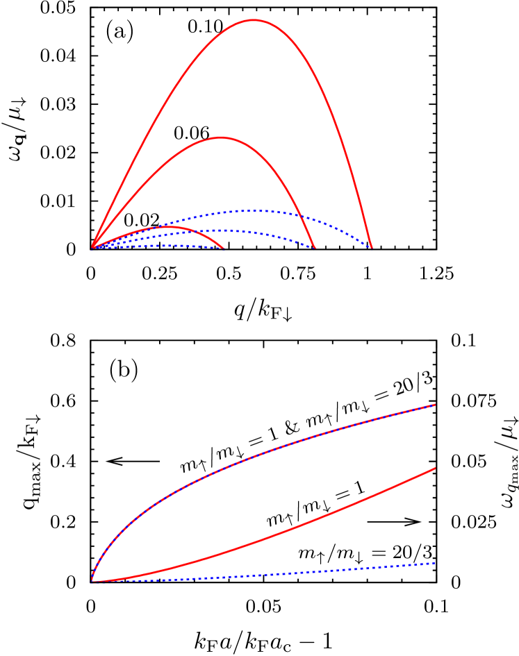
Figure 5: (Color online) (a) shows the growth rate $\omega_{\mathbf{q}}$ as a function of wave vector $q$ for collective modes at values of the dimensionless interaction strength $k_{\text{F}}a/k_{\text{F}}a_{\text{c}}-1=\{0.02,0.06,0.10\}$. Here $k_{\text{F}}a_{\text{c}}$ is the critical interaction strength of the Stoner transition, given in the general mass and population imbalanced case by the boundary in Fig. 1. The solid red curves correspond to the mass balanced gas, and the dashed blue lines to a gas of ⁶Li and ⁴⁰K, where the chemical potentials have been tuned to give population balance at $k_{\text{F}}a=0$. (b) Summarizes the behavior of mode wave vector (primary y-axis) and maximum growth rate (secondary y-axis) in (a). The axes are normalized by the Fermi wave vector and chemical potential of the ⁶Li atoms.

One tactic to reduce three-body losses in the ferromagnetic gas is to study the dynamics immediately following an interaction strength quench. The mass balanced ultracold atomic gas is predicted to form unstable collective modes Babadi09 , and here we explore the mass imbalanced case. To obtain the wave vector $\mathbf{q}$ and growth rate $\omega_{\mathbf{q}}$ of the unstable modes, we search for the poles in the magnetization propagator, which are the solutions to

$$\left(\mathrm{z}\right):\;1-g^{2}\Pi_{\uparrow\uparrow}^{\omega,\mathbf{q}}\Pi_{\downarrow\downarrow}^{\omega,\mathbf{q}} =0$$

$$\left(\perp\right):\;1+\frac{g}{2}\left(\Pi_{\uparrow\downarrow}^{\omega,\mathbf{q}}+\Pi_{\downarrow\uparrow}^{\omega,\mathbf{q}}\right) =0\,.$$ (12)

The growth rate relation for modes along the quantization axis is given by solving $\left(\text{z}\right)$, whereas the relation for perpendicular modes is given by solving $\left(\perp\right)$. The polarization $\Pi_{\alpha\beta}^{\omega,\mathbf{q}}$ is as defined immediately below Eq. (9), except with $g=0$.

We calculate these susceptibilities computationally. In Fig. 5(a) we plot the frequency against wave vector relations for the z direction, and compare those with the mass balanced case. The curves in Fig. 5(a) reveal the most unstable mode with largest growth rate $\omega_{\mathbf{q}}$ has a well defined maximum at wave vector $q=q_{\max}$. In the context of experiment, we expect the domains to be roughly of size $\sim 1/q_{\max}$, and have growth rates $\sim\omega_{q_{\max}}$.

We see in Fig. 5(b) that, for a particular normalized value of the interaction strength, using the ⁶Li-⁴⁰K mass imbalanced system does not affect the size of z domains but does reduce the rate of domain growth by a factor of $\sim 5$ relative to a mass balanced gas. However, in Fig. 4(n) we see that ⁶Li-⁴⁰K three-body losses were suppressed by a factor of $\sim 20$ compared to a mass balanced gas. Therefore, for the same net loss the domains in a mass imbalanced gas can undergo $\sim 4=20/5$ times the growth. For the perpendicular direction, the introduction of mass imbalance decreases domain size, while increasing formation time.

VI Discussion

An ultracold atomic gas of fermions with repulsive interactions offers investigators a new flexible system in which to realize itinerant ferromagnetism. Introducing a mass imbalance between the two spin species drives new distinctive features in the experimental observables of the cloud size, release energy, and loss rate that should help better characterize the formation of a ferromagnetic phase. Furthermore a mass imbalance can strongly suppress the three-body loss rate that plagues the formation of the ferromagnetic phase.

The presence of a mass imbalance also opens up new opportunities to study collective phenomena beyond those that can be realized in the standard Stoner model. Though we showed that a spin textured phase analogous to the Fulde-Ferrell-Larkin-Ovchinnikov state in superconductors is not formed at mean-field level, it has already been established that fluctuations corrections drive its formation even in a mass balanced gas. The presence of a mass imbalance will alter the Fermi surface nesting and could pose an interesting direction for future research.

- (1) W.C. Stwalley, Phys. Rev. Lett. 37, 1628 (1976); E. Tiesinga, B.J. Verhaar, and H.T.C. Stoof, Phys. Rev. A 47, 4114, (1993).
- (2) K.E. Strecker, G.B. Partridge, and R.G. Hulet, Phys. Rev. Lett. 91, 080406 (2003); S. Gupta et al., Science 300, 1723 (2003); C. Chin et al., Science 305, 1128 (2004); C.A. Regal, M. Greiner, and D.S. Jin, Phys. Rev. Lett. 92, 040403 (2004).
- (3) G.-B. Jo et al., Science 325, 1521 (2009).
- (4) D. Pekker et al., Phys. Rev. Lett. 106, 050402 (2011).
- (5) R.A. Duine and A.H. MacDonald, Phys. Rev. Lett. 95, 230403 (2005).
- (6) L.J. LeBlanc, J.H. Thywissen, A.A. Burkov and A. Paramekanti, Phys. Rev. A 80, 013607 (2009).
- (7) G.J. Conduit and B.D. Simons. Phys. Rev. Lett. 103, 200403 (2009).
- (8) M. Houbiers et al., Phys. Rev. A 56, 4864 (1997); L. Salasnich et al., J. Phys. B: At. Mol. Opt. Phys. 33, 3943 (2000); M. Amoruso et al., Eur. Phys. J. D 8, 361 (2000); T. Sogo and H. Yabu, Phys. Rev. A 66, 043611 (2002).
- (9) G.J. Conduit and B.D. Simons, Phys. Rev. A 79, 053606 (2009).
- (10) I. Berdnikov, P. Coleman and S.H. Simon, Phys. Rev. B 79, 224403 (2009);
- (11) G.J. Conduit, E. Altman, Phys. Rev. A 83, 043618 (2011).
- (12) H. Zhai, Phys. Rev. A 80, 051605(R) (2009); X. Cui and H. Zhai, Phys. Rev. A 81, 041602(R) (2010).
- (13) R.A. Duine, M. Polini, H.T.C. Stoof and G. Vignale, Phys. Rev. Lett. 104, 220403 (2010).
- (14) G.J. Conduit and E. Altman, Phys. Rev. A 82, 043603 (2010).
- (15) G.J. Conduit, Phys. Rev. A 82, 043604 (2010).
- (16) B. Wunsch, L. Fritz, N.T. Zinner, E. Manousakis and E. Demler, Phys. Rev. A 81, 013616 (2010); S. Zhang, H.-H. Hung, and C. Wu, Phys. Rev. A 82, 053618 (2010); M. Okumura, S. Yamada, M. Machida and H. Aoki, Phys. Rev. A 83, 031606(R) (2011).
- (17) J.E. Hirsch, Phys. Rev. B 59, 6256 (1999).
- (18) D.S. Petrov, Phys. Rev. A 67, 010703(R) (2003).
- (19) P. Fulde and R.A. Ferrell, Phys. Rev. 135, A550 (1964); A.I. Larkin and Y.N. Ovchinnikov, Sov. Phys. JETP 20, 762 (1965).
- (20) G.J. Conduit, A.G Green and B.D. Simons. Phys. Rev. Lett. 103, 207201 (2009).
- (21) S. Pilati, G. Bertaina, S. Giorgini and M. Troyer, Phys. Rev. Lett. 105, 030405 (2010); S.-Y. Chang, M. Randeria and N. Trivedi, Proceedings of the National Academy of Sciences 108, 51 (2011).
- (22) J.A. Hertz, Phys. Rev. B 14, 1165 (1976).
- (23) E.C. Stoner, Proc. R. Soc. London, Ser. A 165, 372 (1938).
- (24) P. Meystre, Atom Optics (Springer, 2001).
- (25) S.Q. Zhou, D.M. Ceperley, S. Zhang, arXiv:1103.3534 (2011).
- (26) M. Babadi et al., arXiv:0908.3483 (2009).
- (27) J.E. Baarsma, K.B. Gubbels and H.T.C. Stoof, Phys. Rev. A 82, 013624 (2010).