Merging for inhomogeneous finite Markov chains, part II: Nash and log-Sobolev inequalities

Abstract

We study time-inhomogeneous Markov chains with finite state spaces using Nash and logarithmic-Sobolev inequalities, and the notion of $c$-stability. We develop the basic theory of such functional inequalities in the time-inhomogeneous context and provide illustrating examples.

and

t1Supported in part by NSF Grant DMS-06-03886.

t2Supported in part by NSF Grants DMS-06-03886, DMS-03-06194 and by a NSF Postdoctoral Fellowship.

keywordAMSMSC2010 subject classification.

1 Introduction

1.1 Background

This article is part of a series of works where we study quantitative merging properties of time inhomogeneous finite Markov chains. Time inhomogeneity leads to a great variety of behaviors. Moreover, even in rather simple situations, we are at a loss to study how a time inhomogeneous Markov chain might behave. Here, we focus on a natural but restricted type of problem. Consider a sequence of aperiodic irreducible Markov kernels $(K_{i})_{1}^{\infty}$ on a finite set $V$. Let $\pi_{i}$ be the invariant measure of $K_{i}$. Assume that, in a sense to be made precise, all $K_{i}$ and all $\pi_{i}$ are similar and the behavior of the time homogeneous chains driven by each $K_{i}$ separately is understood. Can we then describe the behavior of the time inhomogeneous chain driven by the sequence $(K_{i})_{1}^{\infty}$?

To give a concrete example, on $V_{N}=\{0,\ldots,N\}$, consider a sequence of aperiodic irreducible birth and death chain kernels $K_{i}$, $i=1,2,\ldots,$ with

$$1/4\leq K_{i}(x,y)\leq 3/4\qquad\mbox{if }|x-y|\leq 1$$

and with reversible measure $\pi_{i}$ satisfying $1/4\leq(N+1)\pi_{i}(x)\leq 4$, for all $x\in V_{N}$. What can we say about the behavior of the corresponding time inhomogeneous Markov chain?

Remarkably enough, there is very little known about this question. What can we expect to be true? What can we try to prove? Let $K_{0,n}(x,\cdot)$ denote the distribution, after $n$ steps, of the time inhomogeneous chain described above started at $x$. It is not hard to see that such a chain satisfies a Doeblin type condition that implies

$${\lim_{n\rightarrow\infty}}\|K_{0,n}(x,\cdot)-K_{0,n}(y,\cdot)\|_{\mathrm{TV}}=0.$$

In the absence of a true target distribution and following ADF , we call this property merging. Of course, this does not qualify as a quantitative result. Extrapolating from the behavior of each kernel $K_{i}$ taken individually, we may hope to show that, if $\lim_{N\rightarrow\infty}t_{N}/N^{2}=\infty$ then

$${\lim_{N\rightarrow\infty}}\|K_{0,t_{N}}(x,\cdot)-K_{0,t_{N}}(y,\cdot)\|_{\mathrm{TV}}=0.$$

The aim of this paper and the companion paper SZ3 is to present techniques that apply to this type of problem. The simple minded problem outlined above is actually quite challenging and we will not be able to resolve it here without some additional hypotheses. However, we show how to adapt techniques such as singular values, Nash and log-Sobolev inequalities to time inhomogeneous chains and provide a variety of examples where these tools apply. In SZ3 , we discussed singular value techniques. Here, we focus on Nash and log-Sobolev inequalities. The examples treated here (as well as those treated in SZ3 , SZ-wave ) are quite particular despite the fact that one may believe that the techniques we use are widely applicable. Whether or not such a belief is warranted is a very interesting and, so far, unanswered question. This is deeply related to the notion of $c$-stability that is introduced here and in SZ3 . The examples we present here and in SZ , SZ3 , SZ-wave are about the only existing evidence of successful quantitative analysis of time inhomogeneous Markov chains.

A more detailed introduction to these questions is in SZ3 . The references Ga , SZ discuss singular value techniques in the case of time inhomogeneous chains that admit an invariant distribution [all kernels $K_{i}$ in the sequence $(K_{i})_{1}^{\infty}$ share a common invariant distribution]. Time inhomogeneous random walks on finite groups provide a large collection of such examples (see also MPS for a particularly interesting example: semirandom transpositions). The papers DLM , DMR are also concerned with quantitative results for time inhomogeneous Markov chains. In particular, the techniques developed in DLM are closely related to ours and we will use some of their results concerning the modified logarithmic Sobolev inequality. References on the basic theory of time inhomogeneous Markov chains are Io , Pa , Sen , Sen2 , Son . For a different perspective, see also CH .

A short review of the relevant aspects of the time inhomogeneous Markov chain literature, including the use of “ergodic coefficients” can be found in SZ-berlin . The vast literature on the famous simulated annealing algorithm is not very relevant for our purpose but we refer to DM for a recent discussion. The paper DG concerned with filtering and genetic algorithms describes problems that are related in spirit to the present work.

1.2 Basic notation

Let $V$ be a finite set equipped with a sequence of kernels $(K_{n})_{1}^{\infty}$ such that, for each $n$, $K_{n}(x,y)\geq 0$ and $\sum_{y}K_{n}(x,y)=1$. An associated Markov chain is a $V$-valued random process $X=(X_{n})_{0}^{\infty}$ such that, for all $n$,

$$P(X_{n}=y|X_{n-1}=x,\ldots,X_{0}=x_{0}) = P(X_{n}=y|X_{n-1}=x)$$

$$= K_{n}(x,y).$$

The distribution $\mu_{n}$ of $X_{n}$ is determined by the initial distribution $\mu_{0}$ and given by

$$\mu_{n}(y)=\sum_{x\in V}\mu_{0}(x)K_{0,n}(x,y),$$

where $K_{n,m}(x,y)$ is defined inductively for each $n$ and each $m\geq n$ by

$$K_{n,m}(x,y)=\sum_{z\in V}K_{n,m-1}(x,z)K_{m}(z,y)$$

with $K_{n,n}=I$ (the identity). If we interpret the $K_{n}$’s as matrices, then this definition means that $K_{n,m}=K_{n+1}\cdots K_{m}$. This paper is mostly concerned with the behavior of the measures $K_{0,n}(x,\cdot)$ as $n$ tends to infinity. In the case of time homogeneous chains where all $K_{i}=Q$ are equal, we write $K_{0,n}=Q^{n}$.

Our main interest is in ergodic like properties of time inhomogeneous Markov chains. In general, one does not expect $\mu_{n}=\mu_{0}K_{0,n}$ to converge toward a limiting distribution. Instead, the natural notion is that of merging of measures as discussed in ADF .

Definition 1.1.

Fix a sequence of Markov kernels as above. We say the sequence is merging if for any $x,y,z\in V$,

$$\lim_{n\rightarrow\infty}K_{0,n}(x,z)-K_{0,n}(y,z)=0.$$ (1)

Remark 1.2.

If the sequence $(K_{i})_{1}^{\infty}$ is merging then, for any two starting distributions $\mu_{0},\nu_{0}$, the measures $\mu_{n}=\mu_{0}K_{0,n}$ and $\nu_{n}=\nu_{0}K_{0,n}$ are merging, that is, $\mu_{n}-\nu_{n}\rightarrow 0$. Since we assume the set $V$ is finite, merging is equivalent to ${\lim_{n\rightarrow\infty}}\|K_{0,n}(x,\cdot)-K_{0,n}(y,\cdot)\|_{\mathrm{TV}}=0$. Hence, we also refer to this property as “total variation merging.”

Total variation merging is also referred to as weak ergodicity in the literature and there exists a body of work concerned with understanding when weak ergodicity holds. See, for example, Io , NS , Pa , Rho , Sen . A main tool used to show weak ergodicity is that of contraction coefficients. Furthermore, in FJ , Birkhoff’s contraction coefficient is used to study ratio ergodicity which is equivalent to what we will later call relative-sup merging. However, it should be noted that even for time homogeneous chains Birkhoff coefficients and related methods fail to provide useful quantitative bounds in most cases.

Our goal is to develop quantitative results in the context of time inhomogeneous chains in the spirit of the work of Aldous, Diaconis and others. In these works, precise estimates of the mixing time of ergodic chains are obtained. Typically, a family of Markov chains indexed by a parameter, say $N$, is studied. Loosely speaking, as the parameter $N$ increases, the complexity and size of the chain increases and one seeks bounds that depend on $N$ in an explicit quantitative way. See, for example, Al , BT , Dia , DSh , DS-C , DS-N , DS-L , DS-M , Fill , MT , MP , StF . Efforts in this direction for time inhomogeneous chains are in DLM , DMR , FJ , Ga , Goel , MPS , SZ , SZ3 . Still, there are only a very small number of results and examples concerning the quantitative study of merging as defined above for time inhomogeneous Markov chains so that it is not very clear what kind of results should be expected and what kind of hypotheses are reasonable. We refer the reader to SZ3 for a more detailed discussion.

The following definition is useful to capture the spirit of our study. It indicates that the simplest case we would like to think about is the case when the sequence $K_{i}$ is obtained by deterministic but arbitrary choices between a finite number of kernels $\mathcal{Q}=\{Q_{1},\ldots,Q_{k}\}$.

Definition 1.3.

We say that a set $\mathcal{Q}$ of Markov kernels on $V$ is merging in total variation if for any sequence $(K_{i})_{0}^{\infty}$ with $K_{i}\in\mathcal{Q}$ for all $i$, we have

$$\forall x,y,z\in V\qquad{\lim_{n\rightarrow\infty}}\|K_{0,n}(x,\cdot)-K_{0,n}(y,\cdot)\|_{\mathrm{TV}}=0.$$

In the study of ergodicity of finite Markov chains, the convergence toward the target distribution is measured using various notions of distance between probability measures. These include the total variation distance

$$\|\mu-\nu\|_{\mathrm{TV}}=\sup_{A\subset V}\{\mu(A)-\nu(A)\},$$

the chi-square distance (w.r.t. $\nu$. Note the asymmetry between $\mu$ and $\nu$.)

$$\biggl{(}\sum_{y}\biggl{|}\frac{\mu(y)}{\nu(y)}-1\biggr{|}^{2}\nu(y)\biggr{)}^{1/2},$$

and the relative sup-distance (again, note the asymmetry)

$$\max_{y}\biggl{\{}\biggl{|}\frac{\mu(y)}{\nu(y)}-1\biggr{|}\biggr{\}}.$$

These will be used here to measure merging.

1.3 Merging time

In the quantitative theory of ergodic time homogeneous Markov chains, the notion of mixing time plays a crucial role. For time inhomogeneous chain, we propose to consider the following definitions.

Definition 1.4.

Fix $\varepsilon\in(0,1)$. Given a sequence $(K_{i})_{1}^{\infty}$ of Markov kernels on a finite set $V$, we call max total variation merging time the quantity

$$T_{\mathrm{TV}}(\varepsilon)=\inf\Bigl{\{}n\dvtx{\max_{x,y\in V}}\|K_{0,n}(x,\cdot)-K_{0,n}(y,\cdot)\|_{\mathrm{TV}}<\varepsilon\Bigr{\}}.$$

Definition 1.5.

Fix $\varepsilon\in(0,1)$. We say that a set $\mathcal{Q}$ of Markov kernels on $V$ has max total variation $\varepsilon$-merging time at most $T$ if for any sequence $(K_{i})_{1}^{\infty}$ with $K_{i}\in\mathcal{Q}$ for all $i$, we have $T_{\mathrm{TV}}(\varepsilon)\leq T$, that is,

$$\forall t>T\qquad\max_{x,y\in V}\{\|K_{0,t}(x,\cdot)-K_{0,t}(y,\cdot)\|_{\mathrm{TV}}\}\leq\varepsilon.$$

Of course, merging can be measured in ways other than total variation. Also merging is a bit less flexible than mixing in this respect since there is no reference measure. One very natural and much stronger notion than total variation is relative sup-distance. For time inhomogeneous chains, total variation merging does not necessarily imply relative-sup merging as defined below. See SZ3 .

Definition 1.6.

We say a sequence $(K_{i})_{1}^{\infty}$ of Markov kernels on a finite set $V$ is merging in relative-sup if for all $x,y,z\in V$

$$\lim_{n\rightarrow\infty}\frac{K_{0,n}(x,z)}{K_{0,n}(y,z)}=1$$

with the convention that $0/0=1$ and $a/0=\infty$ for $a>0$. Fix $\varepsilon\in(0,1)$, we call relative-sup merging time the quantity

$$T_{\infty}(\varepsilon)=\inf\biggl{\{}n\dvtx\max_{x,y,z\in V}\biggl{\{}\biggl{|}\frac{K_{0,n}(x,z)}{K_{0,n}(y,z)}-1\biggr{|}\biggr{\}}<\varepsilon\biggr{\}}.$$

Definition 1.7.

We say a set $\mathcal{Q}$ of Markov kernels on $V$ is merging in relative-sup if any sequence $(K_{i})_{1}^{\infty}$ with $K_{i}\in\mathcal{Q}$ for all $i$ is merging in relative-sup.

Fix $\varepsilon\in(0,1)$. We say that $\mathcal{Q}$ has relative-sup $\varepsilon$-merging time at most $T$ if for any sequence $(K_{i})_{1}^{\infty}$ with $K_{i}\in\mathcal{Q}$ for all $i$, we have $T_{\infty}(\varepsilon)\leq T$, that is,

$$\forall t>T\qquad\max_{x,y,z\in V}\biggl{\{}\biggl{|}\frac{K_{0,t}(x,z)}{K_{0,t}(y,z)}-1\biggr{|}\biggr{\}}\leq\varepsilon.$$

The following problem is open. It is a quantitative version of the problem stated at the beginning of the introduction.

Problem 1.8.

Let $V_{N}=\{0,\ldots,N\}$ and $c\in[1,\infty)$. Let $\mathcal{Q}_{N}$ be the set of all birth and death chains $Q$ on $V_{N}$ with $Q(x,y)\in[1/4,3/4]$ if $|x-y|\leq 1$, and reversible measure $\pi$ satisfying $1/4\leq(N+1)\pi(x)\leq 4$, $x\in V_{N}$.

1. Prove or disprove that there exists a constant $A$ independent of $N$ such that $\mathcal{Q}_{N}$ has total variation $\varepsilon$-merging time at most $AN^{2}(1+\log_{+}1/\varepsilon)$.

2. Prove or disprove that there exists a constant $A$ independent of $N$ such that $\mathcal{Q}_{N}$ has relative-sup $\varepsilon$-merging time at most $AN^{2}(1+\log_{+}1/\varepsilon)$.

Remark 1.9.

This problem is open (in most cases) even if one considers a sequence $(K_{i})_{1}^{\infty}$ drawn from a set $\mathcal{Q}=\{K_{1},K_{2}\}$ of two kernels. Observe that the hypothesis that the invariant measures $\pi_{i}$ are all comparable to the uniform plays some role. How to harvest the global hypothesis of comparable stationary distributions $\pi_{i}$ is not entirely clear. See Theorem 1.14 below for a partial solution.

If $\pi_{1}$ and $\pi_{2}$ are not comparable, it is possible for $(K_{1},\pi_{1})$ and $(K_{2},\pi_{2})$ to have the same mixing time yet for $\mathcal{Q}=\{K_{1},K_{2}\}$ to have a merging time of a higher order. Assume that $K_{1}$ and $K_{2}$ are two biased random walks with equal drift, one drift to left, the other to the right. Despite the fact that each of these random walks has a relative-sup mixing time of order $N$, the inhomogeneous chain driven by the sequence $K_{1}K_{2}K_{1}K_{2}\cdots$ has a relative-sup merging time of order $N^{2}$, see SZ3 .

1.4 Stability

In this section, we consider a property, $c$-stability, that plays a crucial role in the techniques we develop to provide quantitative bounds for time inhomogeneous Markov chains. This property was introduced and discussed in SZ3 . It is a straightforward generalization of the property of sharing the same invariant measure. Unfortunately, it is hard to check.

Definition 1.10.

Fix $c\geq 1$. A sequence of Markov kernels $(K_{n})_{1}^{\infty}$ on a finite set $V$ is $c$-stable if there exists a measure $\mu_{0}$ such that

$$\forall n\geq 0,x\in V\qquad c^{-1}\leq\frac{\mu_{n}(x)}{\mu_{0}(x)}\leq c,$$ (2)

where $\mu_{n}=\mu_{0}K_{0,n}$. If this holds, we say that $(K_{n})_{1}^{\infty}$ is $c$-stable with respect to the measure $\mu_{0}$.

Definition 1.11.

A set $\mathcal{Q}$ of Markov kernels is $c$-stable with respect to a measure $\mu_{0}$ if any sequence $(K_{i})_{1}^{\infty}$ such that $K_{i}\in\mathcal{Q}$ for all $i$ is $c$-stable with respect to $\mu_{0}$.

Remark 1.12.

If all $K_{i}$ share the same invariant distribution $\pi$ then $(K_{i})_{1}^{\infty}$ is $1$-stable with respect to $\pi$.

Remark 1.13.

Suppose a set $\mathcal{Q}$ of aperiodic irreducible Markov kernels is $c$-stable with respect to a measure $\mu_{0}$. Let $\pi$ be an invariant measure for some $Q\in\mathcal{Q}$. Then we must have

$$x\in V,\qquad\frac{1}{c}\leq\frac{\pi(x)}{\mu_{0}(x)}\leq c.$$

Hence, $\mathcal{Q}$ is also $c^{2}$-stable with respect to $\pi$ and any two invariant measures $\pi,\pi^{\prime}$ for kernels $Q,Q^{\prime}\in\mathcal{Q}$ must satisfy

$$x\in V,\qquad\frac{1}{c^{2}}\leq\frac{\pi(x)}{\pi^{\prime}(x)}\leq c^{2}.$$

The following theorem which relates to a special case of Problem 1.8 illustrates the role of $c$-stability.

Theorem 1.14

Let $V_{N}=\{0,\ldots,N\}$. Let $\mathcal{Q}_{N}$ be the set of all birth and death chains $Q$ on $V_{N}$ with

$$Q(x,y)\in[1/4,3/4]\qquad\mbox{if }|x-y|\leq 1$$

and reversible measure $\pi$ satisfying $1/4\leq(N+1)\pi(x)\leq 4$, $x\in V_{N}$. Let $(K_{i})_{1}^{\infty}$ be a sequence of birth and death Markov kernels on $V_{N}$ with $K_{i}\in\mathcal{Q}_{N}$. Assume that $(K_{i})_{1}^{\infty}$ is $c$-stable with respect to the uniform measure on $V_{N}$, for some constant $c\geq 1$ independent of $N$. Then there exists a constant $A=A(c)$ (in particular, independent of $N$) such that the relative-sup merging time for $(K_{i})_{1}^{\infty}$ on $V_{N}$ is bounded by

$$T_{\infty}(\varepsilon)\leq AN^{2}(1+\log_{+}1/\varepsilon).$$

This will be proved later in a stronger form in Section 2.4. In SZ3 the weaker conclusion $T_{\infty}(\varepsilon)\leq AN^{2}(\log N+\log_{+}1/\varepsilon)$ was obtained using singular value techniques. Here, we will use Nash inequalities to obtain $T_{\infty}(\varepsilon)\leq AN^{2}(1+\log_{+}1/\varepsilon)$.

It is possible that the set $\mathcal{Q}_{N}$ is $c$-stable with respect to the uniform measure for some $c$. Indeed, it is tempting to conjecture that this is the case although the evidence is rather limited (see also the discussion in SZ-berlin ). If this is true, then Theorem 1.14 solves Problem 1.8. However, we do not know how to approach the problem of proving $c$-stability for $\mathcal{Q}_{N}$.

Remark 1.15.

While the assumption of $c$-stability in Theorem 1.14 is quite strong, Sections 4.2 and 5 of SZ3 give specific examples of families $\mathcal{Q}_{N}$ for which it holds. Further, we note that the question of whether or not $c$-stability holds is extremely natural and interesting in itself.

2 Singular values and Nash inequalities

One key idea in the study of Markov chains is to associate to a Markov kernel $K$ the operator $K\dvtx f\mapsto Kf=\sum_{y}K(\cdot,y)f(y)$. In the case of time homogeneous chains, one uses the basic fact that this operator acts on $\ell^{p}(\pi)$ with norm $1$ when $\pi$ is an invariant measure.

In the case of time inhomogeneous chains, it is crucial to consider $K$ as an operator between $\ell^{p}$ spaces with different measures in the domain and target spaces. The following simple observation is key.

Given a measure $\mu$ and a Markov kernel $K$ on a finite set $V$, set $\mu^{\prime}=\mu K$. Fix $p\in[1,\infty)$ and consider $K$ as a linear operator

$$K=K_{\mu}\dvtx\ell^{p}(\mu^{\prime})\rightarrow\ell^{p}(\mu),\qquad Kf(x)=\sum_{y}K(x,y)f(y).$$ (3)

Then

$$\qquad\|K\|_{\ell^{p}(\mu^{\prime})\rightarrow\ell^{p}(\mu)}=\sup\bigl{\{}\|Kf\|_{\ell^{p}(\mu)}\dvtx f\in\ell^{p}(\mu^{\prime}),\|f\|_{\ell^{p}(\mu^{\prime})}\leq 1\bigr{\}}=1.$$ (4)

This follows from Jensen’s inequality. See, for example, DLM , SZ3 . We will use the notation $K_{\mu}$ whenever we need to emphasize the fact that $K$ is viewed as an operator between $\ell^{p}(\mu K)$ and $\ell^{q}(\mu)$ for some $1\leq p,q\leq\infty$. When the context is clear, we will drop the subscript $\mu$ as was done above.

2.1 Using various distances

Given a sequence of Markov kernels $(K_{i})_{1}^{\infty}$, fix a starting measure $\mu_{0}$ and set $\mu_{n}=\mu_{0}K_{0,n}$. We will assume that $\mu_{n}>0$ for all $n$. Note that if $\mu_{0}>0$ and $K_{n}$ are all irreducible then $\mu_{n}>0$ for all $n\geq 0$. We are interested in the behavior of

$$d_{p}(K_{0,n}(x,\cdot),\mu_{n})=\biggl{(}\sum_{y}\biggl{|}\frac{K_{0,n}(x,y)}{\mu_{n}(y)}-1\biggr{|}^{p}\mu_{n}(y)\biggr{)}^{1/p},\qquad p\geq 1.$$

For $p\geq 1$, a classical argument involving the duality between $\ell^{p}$ and $\ell^{q}$ where $1=1/p+1/q$, yields

$$d_{p}(K_{0,n}(x,\cdot),\mu_{n})=\sup\biggl{\{}\biggl{|}\sum_{y}[K_{0,n}(x,y)f(y)-\mu_{n}(y)f(y)]\biggr{|}\dvtx\|f\|_{\ell^{q}(\mu_{n})}\leq 1\biggr{\}}$$

and one checks that the function

$$n\mapsto d_{p}(K_{0,n}(x,\cdot),\mu_{n})$$

is nonincreasing (see SZ3 ). Of course,

$$2\|K_{0,n}(x,\cdot)-\mu_{n}\|_{\mathrm{TV}}=d_{1}(K_{0,n}(x,\cdot),\mu_{n})$$

and, if $1\leq p\leq r\leq\infty$,

$$d_{p}(K_{0,n}(x,\cdot),\mu_{n})\leq d_{r}(K_{0,n}(x,\cdot),\mu_{n}).$$

In particular,

$$2\|K_{0,n}(x,\cdot)-\mu_{n}\|_{\mathrm{TV}}\leq d_{2}(K_{0,n}(x,\cdot),\mu_{n})$$ (5)

and

$$\|K_{0,n}(x,\cdot)-K_{0,n}(y,\cdot)\|_{\mathrm{TV}}\leq\max_{x\in V}\{d_{2}(K_{0,n}(x,\cdot),\mu_{n})\}.$$ (6)

Further, if

$$\max_{x,z}\biggl{\{}\biggl{|}\frac{K_{0,n}(x,z)}{\mu_{n}(z)}-1\biggr{|}\biggr{\}}\leq\varepsilon\leq 1/2,$$

then

$$\max_{x,y,z}\biggl{\{}\biggl{|}\frac{K_{0,n}(x,z)}{K_{0,n}(y,z)}-1\biggr{|}\biggr{\}}\leq 4\varepsilon.$$

To see the last inequality, note that if $1-\varepsilon\leq a/b,c/b\leq 1+\varepsilon$ with $\varepsilon\in(0,1/2)$ then

$$1-2\varepsilon\leq\frac{1-\varepsilon}{1+\varepsilon}\leq\frac{a}{c}\leq\frac{1+\varepsilon}{1-\varepsilon}\leq 1+4\varepsilon.$$

2.2 Singular values

In SZ3 , we developed basic inequalities for $d_{2}(K_{0,n}(x$, $\cdot),\mu_{n})$ based on singular value decompositions. The basic fact here is that, if $\mu$ is a probability measure on $V$, $K$ a Markov kernel and $\mu^{\prime}=\mu K$ then

$$d_{2}(K(x,\cdot),\mu^{\prime})^{2}=\sum_{i=1}^{|V|-1}|\psi_{i}(x)|^{2}\sigma_{i}^{2},$$

where $\sigma_{i}$, $i=0,\ldots,|V|-1$, are the singular values of $K_{\mu}\dvtx\ell^{2}(\mu^{\prime})\rightarrow\ell^{2}(\mu)$ in nonincreasing order, that is the square root of the eigenvalues of $K_{\mu}K^{*}_{\mu}\dvtx\ell^{2}(\mu)\rightarrow\ell^{2}(\mu)$ where $K^{*}_{\mu}\dvtx\ell^{2}(\mu)\rightarrow\ell^{2}(\mu^{\prime})$ is the adjoint of $K_{\mu}\dvtx\ell^{2}(\mu^{\prime})\rightarrow\ell^{2}(\mu)$. The $\psi_{i}$’s form an orthonormal basis for $\ell^{2}(\mu)$ and are eigenfunctions of $K_{\mu}K^{*}_{\mu}$, $\psi_{i}$ being associated with $\sigma^{2}_{i}$. Of course, the $\sigma_{i}^{2}$’s can also be viewed as the eigenvalues of $K_{\mu}^{*}K_{\mu}\dvtx\ell^{2}(\mu^{\prime})\rightarrow\ell^{2}(\mu^{\prime})$.

In any case, a crucial fact for us here is that $\sigma_{1}$, the second largest singular value of $K_{\mu}\dvtx\ell^{2}(\mu^{\prime})\rightarrow\ell^{2}(\mu)$, is also the norm of $K-\mu^{\prime}=K_{\mu}-\mu^{\prime}\dvtx\ell^{2}(\mu^{\prime})\rightarrow\ell^{2}(\mu)$, that is,

$$\sup\bigl{\{}\|(K-\mu^{\prime})f\|_{\ell^{2}(\mu)}\dvtx f\in\ell^{2}(\mu^{\prime}),\|f\|_{\ell^{2}(\mu^{\prime})}=1\bigr{\}}=\sigma_{1}.$$

Given a sequence $(K_{i})_{1}^{\infty}$ of Markov kernels on $V$ and a positive measure $\mu_{0}$, set $\mu_{n}=\mu_{0}K_{0,n}$ and let $\sigma_{1}(K_{i},\mu_{i-1})$ be the second largest singular value of $K_{i}\dvtx\ell^{2}(\mu_{i})\rightarrow\ell^{2}(\mu_{i-1})$. Noting that

$$(K_{0,n}-\mu_{n})=(K_{1}-\mu_{1})(K_{2}-\mu_{2})\cdots(K_{n}-\mu_{n}),$$

we obtain

$$\|K_{0,n}-\mu_{n}\|_{\ell^{2}(\mu_{n})\rightarrow\ell^{2}(\mu_{0})}\leq\prod_{1}^{n}\sigma_{1}(K_{i},\mu_{i-1}).$$ (7)

This inequality seems very promising and this is rather misleading. There is very little hope to compute or estimate the singular values $\sigma_{i}(K_{i},\mu_{i-1})$, even if we have a good grasp on the kernel $K_{i}$. The reason is that $\sigma_{1}(K_{i},\mu_{i-1})$ depends very much on the unknown measure $\mu_{i-1}$. This is similar to the problem one faces when studying an irreducible aperiodic time homogeneous finite Markov chain for which one is not able to compute the stationary measure (although this case is rarely discussed, it is the typical case). For positive examples and a more detailed discussion, see SZ3 .

2.3 Dirichlet forms

Given a reversible Markov kernel $Q$ with reversible measure $\pi$ on a finite set $V$, the associated Dirichlet form is

$$\mathcal{E}(f,f) = \mathcal{E}_{Q,\pi}(f,f)=\langle(I-Q)f,f\rangle_{\pi}$$

$$= \frac{1}{2}\sum_{x,y}|f(x)-f(y)|^{2}\pi(x)Q(x,y).$$

This definition is essential for the techniques considered in this paper. To illustrate this, we note that the singular value $\sigma_{1}(K_{\mu},\mu)$ associated to a Markov kernel $K$ and a positive probability measure $\mu$ is the square root of the second largest eigenvalue of $K^{*}_{\mu}K_{\mu}\dvtx\ell^{2}(\mu^{\prime})\rightarrow\ell^{2}(\mu^{\prime})$, $\mu^{\prime}=\mu K$. This operator is associated with the Markov kernel

$$P(x,y)=\frac{1}{\mu^{\prime}(x)}\sum_{z}\mu(z)K(z,x)K(z,y),$$

which is reversible with respect to $\mu^{\prime}$ and has associated Dirichlet form

$$\mathcal{E}_{P,\mu^{\prime}}(f,f)=\frac{1}{2}\sum_{x,y,z}|f(x)-f(y)|^{2}\mu(z)K(z,x)K(z,y).$$

Hence, using the classical variational formula for eigenvalues, we have

$$1-\sigma_{1}(K,\mu)=\inf\biggl{\{}\frac{\mathcal{E}_{P,\mu^{\prime}}(f,f)}{\operatorname{Var}_{\mu^{\prime}}(f)}\dvtx f\in\ell^{2}(\mu^{\prime}),\operatorname{Var}_{\mu^{\prime}}(f)\neq 0\biggr{\}},$$

where $\operatorname{Var}_{\mu^{\prime}}(f)=\|f\|^{2}_{\ell^{2}(\mu^{\prime})}-\mu^{\prime}(f)^{2}={\sum_{x}}|f(x)-\mu^{\prime}(f)|^{2}\mu^{\prime}(x)$.

2.4 Nash inequalities

The use of Nash inequalities to study the convergence of ergodic (time homogeneous) finite Markov chains was developed in DS-N (Section 7 of DS-N discusses time homogeneous chains that admits an invariant measure). We refer the reader to that paper for background on this technique. In this section, we observe that it can be implemented in the context of time inhomogeneous chains. We start with some basic material.

Definition 2.1.

Let $V$ be a state space equipped with a Markov kernel $K$ and probability measures $\mu$ and $\nu$. If $1\leq p,q\leq\infty$ then

$$\|K\|_{\ell^{p}(\mu)\rightarrow\ell^{q}(\nu)}=\sup_{\|f\|_{\ell^{p}(\mu)\leq 1}}\bigl{\{}\|Kf\|_{\ell^{q}(\nu)}\bigr{\}}.$$

If $p$ and $q$ are conjugate exponents, that is, if $1/p+1/q=1$, then

$$\|f\|_{\ell^{p}(\mu)}=\sup_{\|g\|_{\ell^{q}(\mu)\leq 1}}\{\langle f,g\rangle_{\mu}\}.$$

The following proposition is well known in a much more general context.

Proposition 2.2

Let $K$ be a Markov kernel. Let $K_{\mu}\dvtx\ell^{2}(\mu K)\rightarrow\ell^{2}(\mu)$ be the Markov operator on $V$ with adjoint $K^{*}_{\mu}\dvtx\ell^{2}(\mu)\rightarrow\ell^{2}(\mu K)$ with respect to the inner product

$$\langle Kf,g\rangle_{\mu}=\langle f,K^{*}g\rangle_{\mu K}.$$

If $1\leq p,r,s\leq\infty$, $1/p+1/q=1$ and $1/r+1/s=1$ then

$$\|K\|_{\ell^{p}(\mu K)\rightarrow\ell^{r}(\mu)}=\|K^{*}\|_{\ell^{s}(\mu)\rightarrow\ell^{q}(\mu K)}.$$

Let now $(K_{i})_{1}^{\infty}$ be a sequence of Markov kernels on $V$. Fix a positive probability measure $\mu_{0}$ and set $\mu_{n}=\mu_{0}K_{0,n}$ as usual. Consider $K_{i}\dvtx\ell^{2}(\mu_{i})\rightarrow\ell^{2}(\mu_{i-1})$, its adjoint $K^{*}_{i}\dvtx\ell^{2}(\mu_{i-1})\rightarrow\ell^{2}(\mu_{i})$ and $P_{i}=K_{i}^{*}K_{i}\dvtx\ell^{2}(\mu_{i})\rightarrow\ell^{2}(\mu_{i})$. The operator $P_{i}$ is given by the Markov kernel

$$P_{i}(x,y)=\frac{1}{\mu_{i}(x)}\sum_{z}\mu_{i-1}(z)K_{i}(z,x)K_{i}(z,y).$$ (8)

This kernel is reversible with reversible measure $\mu_{i}$. We let

$$\mathcal{E}_{P_{i},\mu_{i}}(f,f)=\frac{1}{2}\sum_{x,y}|f(x)-f(y)|^{2}\mu_{i}(x)P_{i}(x,y)$$

be the associated Dirichlet form on $\ell^{2}(\mu_{i})$.

Theorem 2.3

Referring to the setup and notation introduced above, let $N\geq 1$ and assume that there are constants $C,D>0$ such that for $1\leq m\leq N$ the following Nash inequalities hold

$$\forall f\dvtx V\rightarrow\mathbb{R}\qquad\|f\|_{\ell^{2}(\mu_{m})}^{2+1/D} \leq C\biggl{(}\mathcal{E}_{P_{m},\mu_{m}}(f,f)$$

$$\hskip 13.3pt{}+\frac{1}{N}\|f\|_{\ell^{2}(\mu_{m})}^{2}\biggr{)}\|f\|_{\ell^{1}(\mu_{m})}^{1/D}.$$

Then, for $0\leq m\leq n\leq N$,

$$\qquad\max\bigl{\{}\|K_{m,n}\|_{\ell^{2}(\mu_{n})\rightarrow\ell^{\infty}(\mu_{m})},\|K_{m,n}\|_{\ell^{1}(\mu_{n})\rightarrow\ell^{2}(\mu_{m})}\bigr{\}}\leq\biggl{(}\frac{4CB}{n-m+1}\biggr{)}^{D},$$ (10)

where $B=B(D,N)=(1+1/N)(1+\lceil 4D\rceil)$.

Let $(K_{i})_{0}^{\infty}$ be a sequence of Markov kernels on $V$ such that the Nash inequalities (2.3) hold. Pick a function $f$ such that $\|f\|_{\ell^{1}(\mu_{n})}=1$. For $1\leq m\leq n\leq N$ define

$$t_{n}(n-m)=\|K_{m,n}f\|^{2}_{\ell^{2}(\mu_{m})}.$$

Note that for any $n>0$, $(t_{n}(i))_{i=0}^{n}$ is nonincreasing. Indeed, using the contraction property (4), we have

$$t_{n}(i+1) = \|K_{n-i-1,n}f\|^{2}_{\ell^{2}(\mu_{n-i-1})}=\|K_{n-i}K_{n-i,n}f\|_{\ell^{2}(\mu_{n-i-1})}^{2}$$

$$\leq \|K_{n-i,n}f\|_{\ell^{2}(\mu_{n-i})}^{2}=t_{n}(i).$$

Moreover, note that for any $0\leq i-1\leq n\leq N$

$$t_{n}(i)^{1+1/(2D)}\leq C\bigl{(}t_{n}(i)-t_{n}(i+1)+t_{n}(i)/N\bigr{)},$$

where $C$ and $D$ are the constants in (2.3). This follows by applying the Nash inequality to the function $K_{n-i,n}f$. Corollary 3.1 of DS-N then yields that

$$t_{n}(i)\leq\biggl{(}\frac{CB}{i+1}\biggr{)}^{2D},\qquad 0\leq i\leq n\leq N,$$

where $B=B(D,N)=(1+1/N)(1+\lceil 4D\rceil)$. In particular, if $0\leq m\leq n\leq N$,

$$\|K_{m,n}\|_{\ell^{1}(\mu_{n})\rightarrow\ell^{2}(\mu_{m})}\leq\bigl{(}(CB)/(n-m+1)\bigr{)}^{D}.$$

From Proposition 2.2 it follows that, for $0\leq m\leq n\leq N$,

$$\|K_{m,n}^{*}\|_{\ell^{2}(\mu_{m})\rightarrow\ell^{\infty}(\mu_{n})}\leq\bigl{(}(CB)/(n-m+1)\bigr{)}^{D}.$$

Next we bound $\|K_{m,n}^{*}\|_{\ell^{1}(\mu_{m})\rightarrow\ell^{\infty}(\mu_{n})}$ for $0\leq m\leq n\leq N$. Consider the quantity $M(N)$ where

$$M(N)=\max_{0\leq m\leq n\leq N}\bigl{\{}(n-m+1)^{2D}\|K_{m,n}^{*}\|_{\ell^{1}(\mu_{m})\rightarrow\ell^{\infty}(\mu_{n})}\bigr{\}}.$$

Let $l=\lfloor\frac{n-m}{2}\rfloor+m$, so that $0\leq m\leq l\leq n\leq N$. We have

$$\|K_{m,n}^{*}\|_{\ell^{1}(\mu_{m})\rightarrow\ell^{\infty}(\mu_{n})} \leq \|K_{m,l}^{*}\|_{\ell^{1}(\mu_{m})\rightarrow\ell^{2}(\mu_{l})}\|K_{l,n}^{*}\|_{\ell^{2}(\mu_{l})\rightarrow\ell^{\infty}(\mu_{n})}$$

$$\leq \biggl{(}\frac{CB}{n-l+1}\biggr{)}^{D}\|K_{m,l}^{*}\|_{\ell^{1}(\mu_{m})\rightarrow\ell^{2}(\mu_{l})}.$$

Note that for all $0\leq m\leq l\leq N$

$$\|K_{m,l}^{*}\|_{\ell^{1}(\mu_{m})\rightarrow\ell^{2}(\mu_{l})}\leq\|K_{m,l}^{*}\|_{\ell^{1}(\mu_{m})\rightarrow\ell^{\infty}(\mu_{l})}^{1/2}\|K_{m,l}^{*}\|_{\ell^{1}(\mu_{m})\rightarrow\ell^{1}(\mu_{l})}^{1/2}.$$ (11)

This follows from the fact that for any function $f$

$$\|K_{m,l}^{*}f\|_{\ell^{2}(\mu_{l})}\leq\|K_{m,l}^{*}f\|_{\ell^{\infty}(\mu_{l})}^{1/2}\|K_{m,l}^{*}f\|_{\ell^{1}(\mu_{l})}^{1/2}.$$

By (4), we have

$$\|K_{m,n}^{*}\|_{\ell^{1}(\mu_{m})\rightarrow\ell^{\infty}(\mu_{n})} \leq \biggl{(}\frac{CB}{n-l+1}\biggr{)}^{D}\|K_{m,l}^{*}\|_{\ell^{1}(\mu_{m})\rightarrow\ell^{\infty}(\mu_{l})}^{1/2}$$

$$\leq \biggl{(}\frac{CB}{(n-l+1)(l-m+1)}\biggr{)}^{D}M(N)^{1/2}$$

$$\leq \biggl{(}\frac{4CB}{(n-m+1)^{2}}\biggr{)}^{D}M(N)^{1/2}.$$

The last inequality follows from the fact that

$$n-l+1\geq\frac{n-m+1}{2}\quad\mbox{and}\quad l-m+1\geq\frac{n-m+1}{2}.$$

So we have $M(N)\leq(4CB)^{2D}$ and it follows that for all $0\leq m\leq n\leq N$

$$\|K_{m,n}^{*}\|_{\ell^{1}(\mu_{m})\rightarrow\ell^{\infty}(\mu_{n})}\leq\biggl{(}\frac{4CB}{n-m+1}\biggr{)}^{2D}.$$

By duality, we get that

$$\|K_{m,n}\|_{\ell^{1}(\mu_{n})\rightarrow\ell^{\infty}(\mu_{m})}\leq\biggl{(}\frac{4CB}{n-m+1}\biggr{)}^{2D}.$$

Next, we use the Riesz–Thorin interpolation theorem, see SW , page 179, which gives us the desired result.

The next results show how Theorem 2.3 together with the singular value technique of Section 2.2 yields merging results.

Theorem 2.4

Referring to the above setup and notation, let $N\geq 1$ and assume that there are constants $C,D>0$ such that for $1\leq m\leq N$ the Nash inequalities

$$\forall f\dvtx V\rightarrow\mathbb{R}\qquad\|f\|_{\ell^{2}(\mu_{m})}^{2+1/D} \leq C\biggl{(}\mathcal{E}_{P_{m},\mu_{m}}(f,f)+\frac{1}{N}\|f\|_{\ell^{2}(\mu_{m})}^{2}\biggr{)}$$

$${}\times\|f\|_{\ell^{1}(\mu_{m})}^{1/D}$$

hold. Let $\sigma_{1}(K_{m},\mu_{m-1})$ be the second largest singular value of $K_{m}\dvtx\ell^{2}(\mu_{m})\rightarrow\ell^{2}(\mu_{m-1})$, that is, the square root of the second largest eigenvalue of $P_{m}$. Then, for $n>m$, $N\geq m\geq 0$, we have

$$d_{2}(K_{0,n}(x,\cdot),\mu_{n})\leq\biggl{(}\frac{8C(1+\lceil 4D\rceil)}{(m+1)}\biggr{)}^{D}\prod_{m+1}^{n}\sigma_{1}(K_{i},\mu_{i-1}).$$ (13)

Moreover, for any $n=2m+u$, $0\leq m\leq N$, we have

$$\max_{x,y}\biggl{\{}\biggl{|}\frac{K_{0,n}(x,y)}{\mu_{n}(y)}-1\biggr{|}\biggr{\}}\leq\biggl{(}\frac{8C(1+\lceil 4D\rceil)}{(m+1)}\biggr{)}^{2D}\prod_{m+1}^{m+u}\sigma_{1}(K_{i},\mu_{i-1}).$$ (14)

We have

$$\max_{x\in V}\{d_{2}(K_{0,n}(x,\cdot),\mu_{n})^{2}\}=\|K_{0,n}-\mu_{n}\|^{2}_{\ell^{2}(\mu_{n})\rightarrow\ell^{\infty}(\mu_{0})},$$

where $\mu_{n}$ is understood as the expectation operator $f\mapsto\mu_{n}(f)$. Moreover, for any $0\leq m\leq n$,

$$K_{0,n}-\mu_{n}=K_{0,m}(K_{m,n}-\mu_{n}),$$

because $K_{0,m}\mu_{n}f=K_{0,m}\mu_{n}(f)=\mu_{n}(f)$. Hence, for $0\leq m\leq N$,

$$d_{2}(K_{0,n}(x,\cdot),\mu_{n})^{2} \leq \|K_{m,n}-\mu_{n}\|^{2}_{\ell^{2}(\mu_{n})\rightarrow\ell^{2}(\mu_{m})}\|K_{0,m}\|^{2}_{\ell^{2}(\mu_{m})\rightarrow\ell^{\infty}(\mu_{0})}$$

$$\leq \Biggl{(}\prod_{m+1}^{n}\sigma_{1}(K_{i},\mu_{i-1})^{2}\Biggr{)}\biggl{(}\frac{4CB}{m+1}\biggr{)}^{2D}.$$

Using $B=N^{-1}(N+1)(1+\lceil 4D\rceil)$, gives (13). To obtain the stronger result (14), write

$$\max_{x,y\in V}\biggl{\{}\biggl{|}\frac{K_{0,n}(x,y)}{\mu_{n}(y)}-1\biggr{|}\biggr{\}}=\|K_{0,n}-\mu_{n}\|_{\ell^{1}(\mu_{n})\rightarrow\ell^{\infty}(\mu_{0})}$$

and

$$\|K_{0,n}-\mu_{n}\|_{\ell^{1}(\mu_{n})\rightarrow\ell^{\infty}(\mu_{0})}$$

$$\qquad\leq\|K_{n-m,n}\|_{\ell^{1}(\mu_{n})\rightarrow\ell^{2}(\mu_{n-m})}\times\|K_{m,n-m}-\mu_{n-m}\|_{\ell^{2}(\mu_{n-m})\rightarrow\ell^{2}(\mu_{m})}$$

$$\qquad\quad{}\times\|K_{0,m}\|_{\ell^{2}(\mu_{m})\rightarrow\ell^{\infty}(\mu_{0})}.$$

The stated bound (14) follows.

Just as we did for singular values, let us emphasize that the powerful looking results stated in this theorem are actually extremely difficult to apply. Again, the point is that the Dirichlet form $\mathcal{E}_{P_{m},\mu_{m}}$, the space $\ell^{2}(\mu_{m})$, and the singular values $\sigma_{1}(K_{m},\mu_{m-1})$ all involve the unknown sequence of measures $\mu_{n}=\mu_{0}K_{0,n}$, $n=0,\ldots.$ The following subsection gives similar but more applicable results under additional hypotheses involving the notion of $c$-stability.

2.5 Nash inequality under $c$-stability

We state two results that parallel Theorems 5.9 and 5.10 of SZ3 .

Theorem 2.5

Fix $c\in(1,\infty)$. Let $(K_{i})_{1}^{\infty}$ be a sequence of irreducible Markov kernels on a finite set $V$. Assume that $(K_{i})_{1}^{\infty}$ is $c$-stable with respect to a positive probability measure $\mu_{0}$. For each $i$, set $\mu_{0}^{i}=\mu_{0}K_{i}$ and let $\sigma(K_{i},\mu_{0})$ be the second largest singular value of $K_{i}=K_{i,\mu_{0}}$ as an operator from $\ell^{2}(\mu^{i}_{0})$ to $\ell^{2}(\mu_{0})$. Let $P^{0}_{i}=K_{i,\mu_{0}}^{*}K_{i,\mu_{0}}$. Let $N\geq 1$ and assume that there are constants $C,D>0$ such that for $1\leq m\leq N$ the Nash inequalities

$$\quad\forall f\dvtx V\rightarrow\mathbb{R}\qquad\|f\|_{\ell^{2}(\mu^{0}_{m})}^{2+1/D} \leq C\biggl{(}\mathcal{E}_{P^{0}_{m},\mu^{0}_{m}}(f,f)+\frac{1}{N}\|f\|_{\ell^{2}(\mu^{0}_{m})}^{2}\biggr{)}$$

$${}\times\|f\|_{\ell^{1}(\mu^{0}_{m})}^{1/D}$$

holds. Then, for $n>m$, $N\geq m\geq 0$, we have

$$d_{2}(K_{0,n}(x,\cdot),\mu_{n}) \leq \biggl{(}\frac{8Cc^{2+3/2D}(1+\lceil 4D\rceil)}{(m+1)}\biggr{)}^{D}$$

$${}\times\prod_{m+1}^{n}\biggl{(}1-\frac{1-\sigma(K_{i},\mu_{0})^{2}}{c^{2}}\biggr{)}^{1/2}.$$

Moreover, for any $n=2m+u$, $0\leq m\leq N$, we have

$$\max_{x,y}\biggl{\{}\biggl{|}\frac{K_{0,n}(x,y)}{\mu_{n}(y)}-1\biggr{|}\biggr{\}} \leq \biggl{(}\frac{8Cc^{2+3/2D}(1+\lceil 4D\rceil)}{(m+1)}\biggr{)}^{2D}$$

$${}\times\prod_{m+1}^{m+u}\biggl{(}1-\frac{1-\sigma(K_{i},\mu_{0})^{2}}{c^{2}}\biggr{)}^{1/2}.$$

First note that since $\mu_{i-1}/\mu_{0}\in[1/c,c]$, we have $\mu_{0}^{i}/\mu_{i}\in[1/c,c]$. Consider the operator $P_{i}$ with kernel

$$P_{i}(x,y)=\frac{1}{\mu_{i}(x)}\sum_{z}\mu_{i-1}(z)K_{i}(z,x)K_{i}(z,y).$$

By assumption

$$\mu_{i}(x)P_{i}(x,y)\geq c^{-1}\mu_{0}^{i}(x)\biggl{[}\frac{1}{\mu^{i}_{0}(x)}\sum_{z}\mu_{0}(z)K_{i}(z,x)K_{i}(z,y)\biggr{]},$$

where the term in brackets on the right-hand side is the kernel of $P^{0}_{i}$. This kernel has second largest eigenvalue $\sigma(K_{i},\mu_{0})^{2}$. A simple eigenvalue comparison argument yields

$$1-\sigma_{1}(K_{i},\mu_{i-1})^{2}\geq\frac{1}{c^{2}}\bigl{(}1-\sigma(K_{i},\mu_{0})^{2}\bigr{)}.$$

Further, comparison of measures and Dirichlet form yields the Nash inequality

$$\forall f\dvtx V\rightarrow\mathbb{R}\qquad\|f\|_{\ell^{2}(\mu_{m})}^{2+1/D} \leq Cc^{2+3/2D}\biggl{(}\mathcal{E}_{P_{m},\mu_{m}}(f,f)+\frac{1}{N}\|f\|_{\ell^{2}(\mu_{m})}^{2}\biggr{)}$$

$${}\times\|f\|_{\ell^{1}(\mu_{m})}^{1/D}.$$

Together with Theorem 2.4, this gives the stated result.

The next result is based on a stronger hypothesis.

Theorem 2.6

Fix $c\in(1,\infty)$. Let $\mathcal{Q}$ be a family of irreducible aperiodic Markov kernels on a finite set $V$. Assume that $\mathcal{Q}$ is $c$-stable with respect to some positive probability measure $\mu_{0}$.

Let $(K_{i})_{1}^{\infty}$ be a sequence of Markov kernels with $K_{i}\in\mathcal{Q}$ for all $i$. Let $\pi_{i}$ be the invariant measure of $K_{i}$. Let $\tilde{P}_{i}=K_{i}^{*}K_{i}$ where $K_{i}\dvtx\ell^{2}(\pi_{i})\rightarrow\ell^{2}(\pi_{i})$. Let $\sigma_{1}(K_{i})$ be the second largest singular value of $K_{i}$ as an operator on $\ell^{2}(\pi_{i})$. Let $N\geq 1$ and assume that there are constants $C,D>0$ such that for $1\leq m\leq N$ the Nash inequalities

$$\forall f\dvtx V\rightarrow\mathbb{R}\qquad\|f\|_{\ell^{2}(\pi_{m})}^{2+1/D} \leq C\biggl{(}\mathcal{E}_{\tilde{P}_{m},\pi_{m}}(f,f)+\frac{1}{N}\|f\|_{\ell^{2}(\pi_{m})}^{2}\biggr{)}$$

$${}\times\|f\|_{\ell^{1}(\pi_{m})}^{1/D}.$$

Then, for $n>m$, $N\geq m\geq 0$, we have

$$d_{2}(K_{0,n}(x,\cdot),\mu_{n}) \leq \biggl{(}\frac{8Cc^{4+3/D}(1+\lceil 4D\rceil)}{(m+1)}\biggr{)}^{D}$$

$${}\times\prod_{m+1}^{n}\biggl{(}1-\frac{1-\sigma_{1}(K_{i})^{2}}{c^{4}}\biggr{)}^{1/2}.$$

Moreover, for any $n=2m+u$, $0\leq m\leq N$, we have

$$\max_{x,y}\biggl{\{}\biggl{|}\frac{K_{0,n}(x,y)}{\mu_{n}(y)}-1\biggr{|}\biggr{\}}\leq\biggl{(}\frac{8Cc^{4+3/D}(1+\lceil 4D\rceil)}{(m+1)}\biggr{)}^{2D}\prod_{m+1}^{m+u}\biggl{(}1-\frac{1-\sigma_{1}(K_{i})^{2}}{c^{4}}\biggr{)}^{1/2}.$$

Note that the hypothesis that $\mathcal{Q}$ is $c$-stable implies $\pi_{i}/\mu_{j}\in[1/c^{2},c^{2}]$ for all $i,j$. Consider again the operator $P_{i}$ and its kernel

$$P_{i}(x,y)=\frac{1}{\mu_{i}(x)}\sum_{z}\mu_{i-1}(z)K_{i}(z,x)K_{i}(z,y).$$

By assumption

$$\mu_{i}(x)P_{i}(x,y) \geq c^{-2}\pi_{i}(x)\biggl{[}\frac{1}{\pi_{i}(x)}\sum_{z}\pi_{i}(z)K_{i}(z,x)K_{i}(z,y)\biggr{]}$$

$$\geq c^{-2}\pi_{i}(x)\tilde{P}_{i}(x,y).$$

A comparison argument similar to the one used in the previous proof yields the desired result.

3 Examples involving Nash inequalities

This section describes applications of the Nash inequality technique to several examples. All these examples are of the following general type.

(1) There is a basic reversible model $(K,\pi)$ on a space $V_{N}$ (growing with $N$) that is well understood because:

• We have good grasp on the second largest singular value $\sigma_{N}$ of $(K,\pi)$.

• The model $(K,\pi)$ satisfies a good Nash inequality, that is, an inequality of the form

  $$\|f\|^{2+1/D}_{\ell^{2}(\pi)}\leq BT_{N}\biggl{(}\mathcal{E}_{K^{*}K,\pi}(f,f)+\frac{1}{bT_{N}}\|f\|_{\ell^{2}(\pi)}^{2}\biggr{)}\|f\|_{\ell^{1}(\pi)}^{1/D}$$

  with $B,b$ independent of $N$ and $T_{N}\simeq(1-\sigma_{N})^{-1}$. Here, $f\simeq g$ implies that there exist constants $d,D>0$ such that $dg\leq f\leq Dg$.

• Together, the Nash inequality and second largest singular value estimate yield the mixing time estimate

  $$\max_{x,y}\biggl{\{}\biggl{|}\frac{K^{t}(x,y)}{\pi(y)}-1\biggr{|}\biggr{\}}\leq\eta,\qquad t\geq\frac{A(1+\log_{+}1/\eta)}{1-\sigma_{N}},$$

  where $A$ is independent of $N$.

(2) We are given a sequence $(K_{i})_{1}^{\infty}$ or a set $\mathcal{Q}_{N}$ of Markov kernels on $V_{N}$ which satisfies:

• $(K_{i})_{1}^{\infty}$ or $\mathcal{Q}_{N}$ is $c$-stable with respect to a measure $\mu_{0}$ which is either equal or at least comparable to $\pi$.

• The Markov kernels $K_{i}$ or the elements of $\mathcal{Q}_{N}$ are all bounded perturbations of $K$ in the sense that $K_{i}(x,y)/K(x,y)$ is bounded away from $0$ and away from $\infty$ for all $(x,y)\in V_{N}^{2}$. In particular, $K_{i}(x,y)=0$ if and only if $K(x,y)=0$.

Under such circumstances, Theorem 2.5 (or Theorem 2.6) applies and yields the conclusion that the time inhomogeneous Markov chain associated with the sequence $K_{i}$ under investigation has a relative-sup merging time $T_{\infty}(\eta)$ bounded by

$$T_{\infty}(\eta)\leq\frac{A^{\prime}(1+\log_{+}1/\eta)}{1-\sigma_{N}}$$

for some constant $A^{\prime}$ independent of $N$.

The most obvious basic model is, perhaps, the simple random walk on $\mathbb{Z}/N\mathbb{Z}$ (with some holding if $N$ is even to avoid periodicity). This model has $1-\sigma_{N}\simeq 1/N^{2}$ and satisfies the desired Nash inequality with $D=1/4$. The first subsection presents applications to a perturbation of this model.

3.1 Asymmetric perturbation at the middle vertex

In this example, $V_{N}=\mathbb{Z}/p_{N}\mathbb{Z}$ is a finite circle. It will be convenient to enumerate the points in $V_{N}$ by writing $V_{N}=\{-(N-1),\ldots,-1,0,1,\ldots,(N-1),N\}$ if $p_{N}=2N$ and $V_{N}=\{-N,\ldots,-1,0,1,\ldots,N\}$ if $p_{N}=2N+1$. The simple random walk in $V$ has kernel

$$Q(x,y)=\cases{1/2,&\quad if $|x-y|=1$,\cr 0,&\quad otherwise,}$$ (19)

and reversible measure $u\equiv\frac{1}{p_{N}}$. For any $\varepsilon>0$, define the perturbation kernel

$$\Delta_{\varepsilon}(x,y)=\cases{\varepsilon,&\quad if $(x,y)=(0,1)$,\cr-\varepsilon,&\quad if $(x,y)=(0,-1)$,\cr 0,&\quad otherwise.}$$ (20)

For $\varepsilon\in(-1/2,1/2)$, the Markov kernel $Q_{\varepsilon}=Q+\Delta_{\varepsilon}$ is a perturbation of $Q$. See Figure 1.

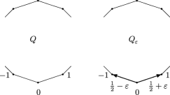
Figure 1: The asymmetric perturbation.

For any fixed $0<\varepsilon<1/2$, set

$$\mathcal{Q}(\varepsilon)=\{Q_{\delta}\dvtx\delta\in[-\varepsilon,\varepsilon]\}.$$

We shall see below that $\mathcal{Q}(\varepsilon)$ is $c$-stable.

Definition 3.1.

Let $\mathcal{S}_{N}(\varepsilon)$ be the set of all probability measures on $V_{N}$ which satisfy the following two properties:

1. [(2)]

2. for all $x\in V_{N}$, there exist constants $a_{\mu,x}$ such that $a_{\mu,x}=-a_{\mu,-x}$ and

   $$\mu(x)=(1/p_{N})+a_{\mu,x}$$

3. for all $x\in V_{N}$ we have that $|a_{\mu,x}|\leq 2\varepsilon/p_{N}$.

Remark 3.2.

Note that we always have $a_{\mu,0}=0$ (since $-0=0$) and, in the case when $p_{N}=2N$, $a_{\mu,N}=0$.

Claim 3.3

Let $\mu\in\mathcal{S}_{N}(\varepsilon)$ defined above, then for any $K\in\mathcal{Q}(\varepsilon)$ we have that $\mu K\in\mathcal{S}_{N}(\varepsilon)$.

Let $\mu\in\mathcal{S}_{N}(\varepsilon)$ and $K=Q_{\delta}\in\mathcal{Q}(\varepsilon)$, $\delta\in[-\varepsilon,\varepsilon]$. We show that $\mu K$ has the properties required to be in $\mathcal{S}_{N}(\varepsilon)$.

(1) Any measure $\mu\in\mathcal{S}_{N}$ can be written as $\mu=u+m_{\mu}$ where $m_{\mu}$ is the (nonprobability) measure $m_{\mu}(x)=a_{\mu,x}$. A simple calculation yields that

$$m_{\mu}Q(x)=(a_{\mu,x-1}+a_{\mu,x+1})/2.$$

Since $a_{\mu,x}=-a_{\mu,-x}$, we obtain that

$$m_{\mu}Q(x)=-m_{\mu}Q(-x)\quad\mbox{and}\quad m_{\mu}Q(0)=0.$$

The fact that $\mu Q=(u+m_{\mu})Q=u+m_{\mu}Q$ implies that $\mu Q$ satisfies property $(1)$ in the definition of $\mathcal{S}_{N}(\varepsilon)$. To see that $\mu Q_{\delta}\in\mathcal{S}_{N}(\varepsilon)$ also satisfies this property, we note that

$$\mu\Delta_{\delta}(x)=\cases{\delta\mu(0),&\quad if $x=1$,\cr-\delta\mu(0),&\quad if $x=-1$,\cr 0,&\quad otherwise.}$$

It now follows that $\mu Q_{\delta}\in\mathcal{S}_{N}$ has property $(1)$ in the definition of $\mathcal{S}_{N}(\varepsilon)$ since $\mu Q_{\delta}=\mu(Q+\Delta_{\delta})$.

(2) We consider the measure $\mu K$. For $x\notin\{-1,1\}$ property $(2)$ of $\mathcal{S}_{N}(\varepsilon)$ follows easily from the fact that $|a_{\mu,x}|\leq 2\varepsilon/p_{N}$ and

$$\mu K(x)=1/p_{N}+1/2(a_{\mu,{x-1}}+a_{\mu,{x+1}}).$$

For $x=1$, we note that

$$\mu K(1) \leq \mu(0)(1/2+\varepsilon)+\mu(2)(1/2)=1/p_{N}+\varepsilon/p_{N}+(1/2)a_{\mu,2}$$

$$\leq 1/p_{N}+2\varepsilon/p_{N}.$$

Similarly

$$\mu K(1) \geq \mu(0)(1/2-\varepsilon)+\mu(2)(1/2)=1/p_{N}-\varepsilon/p_{N}-(1/2)a_{\mu,2}$$

$$\geq 1/p_{N}-2\varepsilon/p_{N}.$$

The proof now follows from the fact that $a_{\mu K,1}=-a_{\mu K,-1}$ as proved in part (1) above.

Claim 3.4

The family $\mathcal{Q}(\varepsilon)$ is $\frac{1+2\varepsilon}{1-2\varepsilon}$-stable with respect to any $\mu_{0}\in\mathcal{S}_{N}(\varepsilon)$.

Claim 3.3 implies that for any sequence $(K_{i})_{0}^{\infty}$ such that $K_{i}\in\mathcal{Q}_{\varepsilon}$ and any measure $\mu_{0}\in\mathcal{S}_{N}(\varepsilon)$ we have $\mu_{n}=\mu_{0}K_{0,n}\in\mathcal{S}_{N}(\varepsilon)$ for all $n\geq 0$. Note that for any measure $\nu\in\mathcal{S}_{N}(\varepsilon)$ we have that

$$\nu(x)=1/p_{N}+a_{\nu,x}\leq(1+2\varepsilon)/p_{N}\quad\mbox{and}\quad\nu(x)=1/p_{N}+a_{\nu,x}\geq(1-2\varepsilon)/p_{N}.$$

Hence,

$$\frac{1-2\varepsilon}{1+2\varepsilon}\leq\frac{\mu_{n}(x)}{\mu_{0}(x)}\leq\frac{1+2\varepsilon}{1-2\varepsilon}.$$

When $p_{N}=2N$, the kernels $Q_{\delta}$ yield periodic chains on $V_{N}$. In this case, we will study the merging properties of

$$\mathcal{Q}_{\mathrm{lazy}}(\varepsilon)=\bigl{\{}\tfrac{1}{2}(I+K)\dvtx K\in\mathcal{Q}(\varepsilon)\bigr{\}},$$

that is, the so-called lazy version of $\mathcal{Q}(\varepsilon)$. We set

$$\overline{Q}_{\delta}=\tfrac{1}{2}(I+Q_{\delta}).$$

For any $\mu\in\mathcal{S}_{N}(\varepsilon)$, we consider the kernel

$$P_{\delta,\mu}(x,y)=\frac{1}{\mu\overline{Q}_{\delta}(x)}\sum_{z}\mu(z)\overline{Q}_{\delta}(z,x)\overline{Q}_{\delta}(z,y),$$

which is the kernel of $K^{*}K$ where $K=\overline{Q}_{\delta}\dvtx\ell^{2}(\mu\overline{Q}_{\delta})\rightarrow\ell^{2}(\mu)$. This is $0$ unless $y=x,x\pm 1,x\pm 2$ and we compare it to

$$P(x,y) = P_{0,u}(x,y)=\frac{1}{u(x)}\sum_{z}u(z)\overline{Q}(z,x)\overline{Q}(z,y)$$

$$= \sum_{z}\overline{Q}(z,x)\overline{Q}(z,y),$$

which is $3/8$ if $y=x$, $1/4$ if $y=x\pm 1$, $1/16$ if $y=x\pm 2$ and $0$ otherwise. The definitions of $Q_{\delta}$ and $\mathcal{S}_{N}(\varepsilon)$ yield

$$\mu\overline{Q}_{\delta}(x)P_{\delta,\mu}(x,y) \geq \frac{(1-2\varepsilon)(1-2\delta)^{2}}{(1+2\varepsilon)}u(x)P(x,y)$$

$$\geq \frac{(1-2\varepsilon)^{3}}{(1+2\varepsilon)}u(x)P(x,y).$$

This yields

$$\mathcal{E}_{P,\mu}(f,f)\leq\frac{(1+2\varepsilon)}{(1-2\varepsilon)^{3}}\mathcal{E}_{P_{\delta,\mu},\mu\overline{Q}_{\delta}}(f,f),$$ (21)

whereas the stability property implies that the relevant measures $\mu\overline{Q}_{\delta}$ and $u$ satisfy

$$\frac{(1-2\varepsilon)}{(1+2\varepsilon)}u\leq\mu\overline{Q}_{\delta}\leq\frac{(1+2\varepsilon)}{(1-2\varepsilon)}u.$$ (22)

In the case when $p_{N}=2N+1$, we may work directly with the kernels $Q_{\delta}$ as they are not periodic. An analysis similar to that above will give versions of (21) and (22) for $Q_{\delta}$.

Applying the line of reasoning explained at the beginning of this section and using Theorem 2.6, we get the following result.

Theorem 3.5

Fix $\varepsilon\in(0,1/2)$. For any $\eta>0$ the total variation $\eta$-merging time of the family $\mathcal{Q}_{\mathrm{lazy}}(\varepsilon)$ on $V_{N}=\mathbb{Z}/2N\mathbb{Z}$ [resp., $\mathcal{Q}(\varepsilon)$ on $V_{N}=\mathbb{Z}/(2N+1)\mathbb{Z}$] is at most $B(\varepsilon)N^{2}(1+\log_{+}1/\eta)$ for some constant $B(\varepsilon)\in(0,\infty)$. In fact, we can choose $B(\varepsilon)$ such that

$$\forall n\geq B(\varepsilon)N^{2}(1+\log_{+}1/\eta)\qquad\max_{x,y\in V_{N}}\biggl{\{}\biggl{|}\frac{K_{0,n}(x,z)}{K_{0,n}(y,z)}-1\biggr{|}\biggr{\}}\leq\eta$$

for any sequence $K_{i}\in\mathcal{Q}_{\mathrm{lazy}}(\varepsilon)$ [resp., $K_{i}\in\mathcal{Q}(\varepsilon)$].

3.2 Perturbations of some birth and death chains

In SC-N , Nash inequalities are used to study certain birth and death chains on $V_{N}=\{-N,\ldots,0,\break\ldots,N\}$ with reversible measures which belong to one of the following two families:

$$\hat{\pi}_{\alpha}(x)=\hat{c}(\alpha,N)(N-|x|+1)^{\alpha},\qquad\alpha\geq 0,$$

and

$$\check{\pi}_{\alpha}(x)=\check{c}(\alpha,N)(|x|+1)^{\alpha},\qquad\alpha\geq 0.$$

Here, we consider $\alpha\in[0,\infty)$ to be a fixed parameter and are interested in what happens when $N$ tends to infinity. From this perspective, the normalizing constants $\hat{c}(\alpha,N),\check{c}(\alpha,N)$ are comparable and behave as

$$\hat{c}(\alpha,N)\simeq\check{c}(\alpha,N)\simeq N^{-\alpha-1}.$$

Set

$$\zeta(\alpha,N)=\sum_{0}^{N}(1+i)^{-\alpha}\simeq\cases{1,&\quad if $\alpha>1$,\cr\log N,&\quad if $\alpha=1$,\cr N^{-\alpha+1},&\quad if $\alpha\in[0,1)$.}$$

Here, all $\simeq$ must be understood for fixed $\alpha$ and the implied comparison constants depend on $\alpha$. Let $\hat{M}_{\alpha}$ (resp., $\check{M}_{\alpha}$) be the Markov kernel of the Metropolis chain with basis the symmetric simple random walk on $V_{N}$ with holding $1/3$ at all points except at the end points where the holding is $2/3$, and target $\hat{\pi}_{\alpha}$, (resp., $\check{\pi}_{\alpha}$). Let $\hat{\lambda}(\alpha,N)$, $\check{\lambda}(\alpha,N)$ be the corresponding spectral gaps. Let $\hat{T}(\alpha,N,\eta)$, $\check{T}(\alpha,N,\eta)$ be the relative-sup mixing times of these chains. It is proved in SC-N that

$$\hat{\lambda}(\alpha,N)\simeq 1/N^{2},\qquad\hat{T}(\alpha,N,\eta)\simeq N^{2}(1+\log_{+}1/\eta),$$

whereas

$$\check{\lambda}(\alpha,N) \simeq \check{c}(\alpha,N)/\zeta(\alpha,N),$$

$$\check{T}(\alpha,N,\eta) \simeq \bigl{(}N^{2}+[\check{c}(\alpha,N)/\zeta(\alpha,N)]\log_{+}1/\eta\bigr{)}.$$

Note that

$$\check{c}(\alpha,N)/\zeta(\alpha,N)\simeq\cases{N^{-(1+\alpha)},&\quad if $\alpha>1$,\cr(N^{2}\log N)^{-1},&\quad if $\alpha=1$,\cr N^{-2},&\quad if $\alpha\in[0,1)$.}$$

These results are based on the Nash inequalities satisfied by these chains. Namely, letting $\mathcal{E}_{\alpha}=\mathcal{E}_{\hat{M}_{\alpha},\hat{\pi}_{\alpha}}$ or $\mathcal{E}_{\alpha}=\mathcal{E}_{\check{M}_{\alpha},\check{\pi}_{\alpha}}$ and $\pi_{\alpha}=\hat{\pi}_{\alpha}$ or $\pi_{\alpha}=\check{\pi}_{\alpha}$, there are constants $A_{\alpha},a_{\alpha}\in(0,\infty)$ such that

$$\|f\|_{\ell^{2}(\pi_{\alpha})}^{2+1/D_{\alpha}}\leq A_{\alpha}N^{2}\biggl{(}\mathcal{E}_{\alpha}(f,f)+\frac{1}{a_{\alpha}N^{2}}\|f\|^{2}_{\ell^{2}(\pi_{\alpha})}\biggr{)}\|f\|_{\ell^{1}(\pi_{\alpha})}^{1/D_{\alpha}}$$

with $D_{\alpha}=1+\alpha$. See SC-N .

In cite SZ3 , the authors consider the class of birth and death chains $Q$ on $V_{N}=\{-N,\ldots,0,\ldots,N\}$ that are symmetric with respect to the middle point, that is, satisfy $Q(x,x+1)=Q(-x,-x-1)$, $Q(x,x-1)=Q(-x,-x+1)$, $Q(x,x)=Q(-x,-x)$, $x\in\{0,N\}$. For any such chain $Q$, let $\nu$ be the reversible measure. It satisfies $\nu(x)=\nu(-x)$. Consider the perturbation set

$$\mathcal{Q}_{N}(Q,\varepsilon)=\{Q+\Delta_{s}\dvtx s\in[-\varepsilon,\varepsilon]\},\qquad\varepsilon\in[0,q_{0}),$$

where $q_{0}=Q(0,\pm 1)$, $\Delta_{s}(0,\pm 1)=\pm s$ and $\Delta(x,y)=0$ otherwise. These perturbations at the middle vertex have reversible measure $\nu_{s}$ that satisfy

$$\nu_{s}(0)=\nu(0),\qquad\nu_{s}(\pm x)=\nu(\pm x)(1\pm s/q_{0}),\qquad x\in\{1,\ldots,N\}.$$

The main point of this construction is the following.

Proposition 3.6

Fix $Q$, $\nu$ as above and $\varepsilon\in[0,q_{0})$. The set $\mathcal{Q}_{N}(Q,\varepsilon)$ is $c$-stable with respect to $\mu_{0}=\nu$ with $c=(q_{0}+\varepsilon)/(q_{0}-\varepsilon)$.

In order to apply this results to our example $\hat{M}_{\alpha},\check{M}_{\alpha}$, we observe that

$$\hat{q}_{0}(\alpha)=\hat{M}_{\alpha}(0,-1)=\frac{1}{3}\biggl{(}\frac{N}{N+1}\biggr{)}^{\alpha}$$

and

$$\check{q}_{0}(\alpha)=\check{M}_{\alpha}(0,-1)=\tfrac{1}{3}.$$

Now, Theorem 2.6 yields the following result.

Theorem 3.7

Fix $\alpha\in[0,\infty)$ and set $\hat{\varepsilon}_{N,\alpha}=\frac{1}{6}(N/(N+1))^{\alpha}$, $\check{\varepsilon}_{N,\alpha}=1/6$.

1. There exists a constant $A$ independent of $N$ such that, for any sequence $(K_{i})_{1}^{\infty}$ with $K_{i}\in\mathcal{Q}_{N}(\hat{M}_{\alpha},\hat{\varepsilon}_{N,\alpha})$, we have

   $$T_{\infty}(\eta)\leq AN^{2}(1+\log_{+}1/\eta).$$

2. There exists a constant $A$ independent of $N$ such that, for any sequence $(K_{i})_{1}^{\infty}$ with $K_{i}\in\mathcal{Q}_{N}(\check{M}_{\alpha},\check{\varepsilon}_{N,\alpha})$, we have

   $$T_{\infty}(\eta)\leq A\cases{N^{2}+N^{1+\alpha}\log_{+}1/\eta,&\quad if $\alpha>1$,\cr N^{2}+(N^{2}\log N)\log_{+}1/\eta,&\quad if $\alpha=1$,\cr N^{2}(1+\log_{+}1/\eta),&\quad if $\alpha\in(0,1)$.}$$

4 Logarithmic Sobolev inequalities

This section develops the technique of logarithmic Sobolev inequality for time inhomogeneous finite Markov chains. It should be noted that the logarithmic Sobolev technique has been mostly applied in the literature in the context of continuous time chains. In Mic , Miclo tackled the problem of adapting this technique to discrete time (time homogeneous) chains. There are two different ways to use logarithmic Sobolev inequality for mixing estimates. One, the most powerful, provides results for relative-sup merging and is based on hypercontractivity. The other is based on entropy and only produces bounds for total variation merging. We will discuss and illustrate both approaches below in the context of time inhomogeneous chains. The entropy approach is already treated in DLM .

4.1 Hypercontractivity

Recall that, for any positive probability distribution $\mu$, a Markov kernel $K$ can be thought of as a contraction

$$K_{\mu}\dvtx\ell^{2}(\mu^{\prime})\rightarrow\ell^{2}(\mu)\qquad\mbox{for $\mu^{\prime}=\mu K$.}$$

The adjoint $K_{\mu}^{*}\dvtx\ell^{2}(\mu)\rightarrow\ell^{2}(\mu^{\prime})$ has kernel

$$K^{*}_{\mu}(x,y)=\frac{K(y,x)\mu(y)}{\mu^{\prime}(x)}.$$

Set $P=K_{\mu}^{*}K_{\mu}\dvtx\ell^{2}(\mu^{\prime})\rightarrow\ell^{2}(\mu^{\prime})$. We define the logarithmic Sobolev constant

$$l(P)=\inf\biggl{\{}\frac{\mathcal{E}_{P,\mu^{\prime}}(f,f)}{\mathcal{L}(f^{2},\mu^{\prime})}\dvtx\mathcal{L}(f^{2},\mu^{\prime})\neq 0,f\neq\mbox{constant}\biggr{\}},$$

where the $\ell^{2}$ relative entropy $\mathcal{L}(f^{2},\nu)$ of a function $f$ with respect to the measure $\nu$ is defined by

$$\mathcal{L}(f^{2},\nu)=\sum_{x\in V}f^{2}\log\biggl{(}\frac{f^{2}}{\|f\|^{2}_{\ell^{2}(\nu)}}\biggr{)}\nu(x).$$

The following proposition is a slight generalization of Mic , Proposition 2, in that it allows for the necessary change of measure.

Proposition 4.1

Let $K$ and $\mu$ be a Markov kernel and a probability measure, respectively. For all $q_{0}\geq 2$ and $q\leq[1+l(P)]q_{0}$, then

$$\|K\|_{\ell^{q_{0}}(\mu^{\prime})\rightarrow\ell^{q}(\mu)}\leq 1.$$

In order to prove the proposition above, we will need the following two lemmas from Mic .

Lemma 4.2 ((Mic , Lemma 3))

Let $\nu$ be a probability measure. For all $q\geq\break q_{0}\geq 1$,

$$\|f\|_{\ell^{q}(\nu)}-\|f\|_{\ell^{q_{0}}(\nu)}\leq\frac{q-q_{0}}{q_{0}q}\|f\|_{\ell^{q}(\nu)}^{1-q}\mathcal{L}(f^{q/2},\nu).$$

Lemma 4.3 ((Mic , Lemma 4))

Fix $\nu\geq 0$ and $q\geq 2$, then for any $t\geq 0$ and $-t\leq s\leq\nu t$ we have that

$$(t+s)^{q}\geq t^{q}+qt^{q-1}s+g(q,\nu)\bigl{(}(t+s)^{q/2}-t^{q/2}\bigr{)}^{2},$$

where

$$g(q,v)=\frac{(1+\nu)^{q}-1-q\nu}{((1+\nu)^{q/2}-1)^{2}}.$$

The proof of Proposition 4.1 follows directly that of Proposition 2 in Mic . Proof of Proposition 4.1 To prove Proposition 4.1 is suffices to only consider positive functions. For $f>0$, we begin by writing

$$\|Kf\|_{\ell^{q}(\mu)}-\|f\|_{\ell^{2}(\mu^{\prime})} = \|Kf\|_{\ell^{q}(\mu)}-\|f\|_{\ell^{q}(\mu^{\prime})}$$

$${}+\|f\|_{\ell^{q}(\mu^{\prime})}-\|f\|_{\ell^{2}(\mu^{\prime})}.$$

The difference of the last two terms on the right-hand side is controlled by Lemma 4.2. To control the first two terms, we will use the concavity result

$$\forall a,b\geq 0\qquad a^{1/q}-b^{1/q}\leq\frac{1}{q}b^{1/q-1}(a-b).$$

It follows that

$$\|Kf\|_{\ell^{q}(\mu)}-\|f\|_{\ell^{q}(\mu^{\prime})}\leq\frac{1}{q}\|f\|_{\ell^{q}(\mu^{\prime})}^{1-q}\bigl{(}\|Kf\|_{\ell^{q}(\mu)}^{q}-\|f\|_{\ell^{q}(\mu^{\prime})}^{q}\bigr{)}.$$

Set

$$\nu(K)=\max\{1/K(x,y)\dvtx K(x,y)>0\}-1.$$

Following the notation of Lemma 4.3, fix $x,y\in V$ and set $\nu=\nu(K)$, $t=Kf(x)$ and $t+s=f(y)$. If $K(x,y)>0$, then $-t\leq s\leq\nu t$ and so

$$f(y)^{q} \geq Kf(x)^{q}+qKf(x)^{q-1}\bigl{(}f(y)-Kf(x)\bigr{)}$$

$${}+g(q,\nu(K))\bigl{(}f(y)^{q/2}-Kf(x)^{q/2}\bigr{)}^{2}.$$

Fix $x$ and integrate with respect to the measure $K(x,\cdot)$ to get

$$Kf^{q}(x)\geq(Kf(x))^{q}+g(q,\nu(K))\sum_{y\in V}K(x,y)\bigl{(}f(y)^{q/2}-Kf(x)^{q/2}\bigr{)}^{2}.$$

We also have

$$\sum_{y\in V}K(x,y)\bigl{(}f^{q/2}(y)-(Kf(x))^{q/2}\bigr{)}^{2} \geq \min_{c\in\mathbb{R}}\sum_{y\in V}K(x,y)\bigl{(}f^{q/2}(y)-c\bigr{)}^{2}$$

$$= \sum_{y\in V}K(x,y)\bigl{(}f^{q/2}(y)-K(f^{q/2})(x)\bigr{)}^{2}$$

$$= Kf^{q}(x)-(Kf^{q/2}(x))^{2}.$$

Hence,

$$Kf^{q}(x)\geq(Kf(x))^{q}+g(q,\nu(K))\bigl{(}Kf^{q}(x)-(Kf^{q/2}(x))^{2}\bigr{)}.$$

Integrating with respect to $\mu$ gives us that

$$\|f\|_{\ell^{q}(\mu^{\prime})}^{q}\geq\|Kf\|_{\ell^{q}(\mu)}^{q}+g(q,\nu(K))\mathcal{E}_{P,\mu^{\prime}}(f^{q/2},f^{q/2}).$$ (24)

It follows from Lemma 4.2, (4.1) and (24) that

$$\|Kf\|_{\ell^{q}(\mu)}-\|f\|_{\ell^{2}(\mu^{\prime})}$$

$$\qquad\leq\frac{1}{q}\|f\|_{\ell^{q}(\mu^{\prime})}^{1-q}\biggl{(}\frac{q-q_{0}}{q_{0}}\mathcal{L}(f^{q/2},\mu^{\prime})-g(q,\nu(K))\mathcal{E}_{P,\mu^{\prime}}(f^{q/2},f^{q/2})\biggr{)}.$$

In Mic , it is noted that for all $\nu>0$ and $q\geq 2$ we have $g(q,\nu)\geq 1$. So if $q\leq[1+l(P)]q_{0}$ then $q\leq[1+g(q,\nu(K))l(P)]q_{0}$. Hence,

$$\|Kf\|_{\ell^{q}(\mu)}-\|f\|_{\ell^{2}(\mu^{\prime})}$$

$$\qquad\leq\frac{1}{q}\|f\|_{\ell^{q}(\mu^{\prime})}^{1-q}g(q,\nu(K))\bigl{(}l(P)\mathcal{L}(f^{q/2},\mu^{\prime})-\mathcal{E}_{P,\mu^{\prime}}(f^{q/2},f^{q/2})\bigr{)}.$$

Since $l(P)$ is the logarithmic Sobolev constant, we get our desired result,

$$\|Kf\|_{\ell^{q}(\mu)}-\|f\|_{\ell^{2}(\mu^{\prime})}\leq 0.$$

Corollary 4.4

Let $(K_{n})_{0}^{\infty}$ be a sequence of Markov kernels on a finite set $V$ and $\mu_{0}$ be an initial distribution on $V$. Set $\mu_{n}=\mu_{0}K_{0,n}$. Consider $K_{i}\dvtx\ell^{2}(\mu_{i})\rightarrow\ell^{2}(\mu_{i-1})$ and $P_{i}=K_{i}^{*}K_{i}\dvtx\ell^{2}(\mu_{i})\rightarrow\ell^{2}(\mu_{i})$. Let $l(P_{i})$ be the logarithmic Sobolev constant of $P_{i}$. Then for any $q_{0}\geq 2$ and $q\leq\prod_{i=1}^{n}(1+l(P_{i}))q_{0}$, we have that

$$\|K_{0,n}\|_{\ell^{q_{0}}(\mu_{n})\rightarrow\ell^{q}(\mu_{0})}\leq 1.$$

When $n=2$, set $q_{1}=(1+l(P_{2}))q_{0}$, then $q=(1+l(P_{1}))q_{1}$. It follows from Proposition 4.1 that

$$\|K_{0,2}\|_{\ell^{q_{0}}(\mu_{2})\rightarrow\ell^{q}(\mu_{0})}\leq\|K_{2}\|_{\ell^{q_{0}}(\mu_{2})\rightarrow\ell^{q_{1}}(\mu_{1})}\|K_{1}\|_{\ell^{q_{1}}(\mu_{1})\rightarrow\ell^{q_{2}}(\mu_{0})}\leq 1.$$

The proof by induction follows similarly.

We now relate the results above to bounds on merging times.

Theorem 4.5

Let $V$ be a finite set equipped with a sequence of Markov kernels $(K_{n})_{0}^{\infty}$ and an initial distribution $\mu_{0}$. Let $\mu_{n}=\mu_{0}K_{0,n}$. Consider $K_{i}\dvtx\break\ell^{2}(\mu_{i})\rightarrow\ell^{2}(\mu_{i-1})$ and $P_{i}=K_{i}^{*}K_{i}\dvtx\ell^{2}(\mu_{i})\rightarrow\ell^{2}(\mu_{i})$. Let $l(P_{i})$ be the logarithmic Sobolev constant of $P_{i}$. Set

$$m_{x}=\min\Biggl{\{}t\in\mathbb{N}\dvtx\sum_{i=1}^{t}\log\bigl{(}1+l(P_{i})\bigr{)}\geq\log\log(\mu_{0}(x)^{-1/2})\Biggr{\}}.$$

Then for $n\geq m_{x}$, we have that

$$d_{2}(K_{0,n}(x,\cdot),\mu_{n})^{2}\leq e^{2}\prod_{i=m_{x}+1}^{n}\sigma_{1}(K_{i},\mu_{i-1})^{2}.$$

Fix $x$, and let $m=m_{x}$. If $0\leq m\leq n$, $K_{0,n}^{*}=K_{m,n}^{*}K_{0,m}^{*}$. Indeed, for any $f\in\ell^{2}(\mu_{0})$ and $g\in\ell^{2}(\mu_{n})$ we have that

$$\langle K_{0,n}^{*}f,g\rangle_{\mu_{n}}=\langle f,K_{0,n}g\rangle_{\mu_{0}}=\langle K_{0,m}^{*}f,K_{m,n}g\rangle_{\mu_{m}}=\langle K_{m,n}^{*}K_{0,m}^{*}f,g\rangle_{\mu_{n}}.$$

Moreover, if $\mu_{m}$ is thought of as the expectation operator $\mu_{m}\dvtx\ell^{2}(\mu_{m})\rightarrow\ell^{2}(\mu_{n})$, $f\mapsto\mu_{m}(f)$, then $(K_{m,n}^{*}-\mu_{m})^{*}=K_{m,n}-\mu_{n}$. Let

$$\delta_{x}(z)=\cases{\mu_{0}(x)^{-1},&\quad if $z=x$,\cr 0,&\quad otherwise.}$$

Set $q=q(m)=2\prod_{i=1}^{m}(1+l(P_{i}))$ and $q^{\prime}(m)$ to be the conjugate exponent of $q(m)$ so that $1/q(m)+1/q^{\prime}(m)=1$. By duality, we have

$$d_{2}(K_{0,n}(x,\cdot),\mu_{n})$$

$$\qquad=\biggl{\|}\frac{K_{0,n}(x,\cdot)}{\mu_{n}(\cdot)}-1\biggr{\|}_{\ell^{2}(\mu_{n})}=\biggl{\|}\frac{K_{0,n}^{*}(\cdot,x)}{\mu_{0}(x)}-1\biggr{\|}_{\ell^{2}(\mu_{n})}$$

$$\qquad=\|(K_{0,n}^{*}-\mu_{0})\delta_{x}\|_{\ell^{2}(\mu_{n})}=\|(K_{m,n}^{*}-\mu_{m})K_{0,m}^{*}\delta_{x}\|_{\ell^{2}(\mu_{n})}$$

$$\qquad\leq\|K_{m,n}^{*}-\mu_{m}\|_{\ell^{2}(\mu_{m})\rightarrow\ell^{2}(\mu_{n})}\|K_{0,m}^{*}\delta_{x}\|_{\ell^{2}(\mu_{m})}$$

$$\qquad\leq\|\delta_{x}\|_{\ell^{q^{\prime}(m)}(\mu_{0})}\|K_{0,m}^{*}\|_{\ell^{q^{\prime}(m)}(\mu_{0})\rightarrow\ell^{2}(\mu_{m})}\|K_{m,n}^{*}-\mu_{m}\|_{\ell^{2}(\mu_{m})\rightarrow\ell^{2}(\mu_{n})}$$

$$\qquad\leq\mu_{0}(x)^{-1/q(m)}\|K_{0,m}\|_{\ell^{2}(\mu_{m})\rightarrow\ell^{q(m)}(\mu_{0})}\|K_{m,n}-\mu_{n}\|_{\ell^{2}(\mu_{n})\rightarrow\ell^{2}(\mu_{m})}.$$

By assumption, we have that $q(m)\geq\log(\mu_{0}(x)^{-1})$, it now follows from Corollary 4.4 that

$$d_{2}(K_{0,n}(x,\cdot),\mu_{n})\leq e\prod_{i=m+1}^{n}\sigma_{1}(K_{i},\mu_{i-1}).$$

4.2 Logarithmic Sobolev inequalities and $c$-stability

Theorem 4.6

Fix $c\in(1,\infty)$. Let $V$ be a finite set equipped with a sequence of irreducible Markov kernels, $(K_{i})_{1}^{\infty}$. Assume that $(K_{i})_{1}^{\infty}$ is $c$-stable with respect to a positive probability measure $\mu_{0}$. For each $i$, set $\mu_{0}^{i}=\mu_{0}K_{i}$ and let $\sigma_{1}(K_{i},\mu_{0})$ be the second largest singular value of the operator $K_{i}\dvtx\ell^{2}(\mu_{0}^{i})\rightarrow\ell^{2}(\mu_{0})$ and $l(K_{i}^{*}K_{i})$ the logarithmic Sobolev constant for the operator $K_{i}^{*}K_{i}\dvtx\ell^{2}(\mu_{0}^{i})\rightarrow\ell^{2}(\mu_{0}^{i})$. If

$$\tilde{m}_{x}=\min\Biggl{\{}t\in\mathbb{N}\dvtx\sum_{i=1}^{t}\log\bigl{(}1+c^{-2}l(K_{i}^{*}K_{i})\bigr{)}\geq\log\log(\mu_{0}(x)^{-1/2})\Biggr{\}},$$

then for $n\geq\tilde{m}_{x}$ we have that

$$d_{2}(K_{0,n}(x,\cdot),\mu_{n})^{2}\leq e^{2}\prod_{i=\tilde{m}_{x}+1}^{n}\bigl{(}1-c^{-2}\bigl{(}1-\sigma_{1}(K_{i},\mu_{0}^{i})^{2}\bigr{)}\bigr{)}.$$

First, we note that $\mu_{i}/\mu_{0}^{i}\in[c^{-1},c]$. Let $P_{i}$ be the Markov kernel described in the statement of Theorem 4.5. By the same arguments as in Theorem 2.5, we get that for all $x,y\in V$

$$\mu_{i}(x)P_{i}(x,y)=\sum_{z}\mu_{i-1}(z)K_{i}(z,x)K_{i}(z,y)\geq c^{-1}\mu_{0}^{i}(x)K_{i}^{*}K_{i}(x,y).$$

A simple comparison argument similar to those used in the proof of Theorem 2.5 (see also DS-C , DS-L ) yields that

$$l(P_{i})\geq c^{-2}l(K_{i}^{*}K_{i})\quad\mbox{and}\quad 1-\sigma(K_{i},\mu_{i-1})^{2}\geq c^{-2}\bigl{(}1-\sigma(K_{i},\mu_{0}^{i})^{2}\bigr{)}.$$

The first inequality implies that $\tilde{m}_{x}\geq m_{x}$ where $m_{x}$ is defined in the proof of Theorem 4.5. Using the results of Theorem 4.5 and the second inequality above gives the desired result.

The next result is when we have a $c$-stability assumption on a family of kernels.

Theorem 4.7

Let $c\in(1,\infty)$. Let $\mathcal{Q}$ be a family of irreducible aperiodic Markov kernels on a finite set $V$. Assume that $\mathcal{Q}$ is $c$-stable with respect to some positive probability measure $\mu_{0}$. Let $(K_{i})_{1}^{\infty}$ be a sequence of Markov kernels with $K_{i}\in\mathcal{Q}$ for all $i$. Let $\pi_{i}$ be the invariant measure of $K_{i}$. Let $\sigma_{i}(K_{i})$ be the second largest singular value for the operator $K_{i}\dvtx\ell^{2}(\pi)\rightarrow\ell^{2}(\pi)$. Let $l(K_{i}^{*}K_{i})$ be the logarithmic Sobolev constant for the operator $K_{i}^{*}K_{i}$ where $K_{i}^{*}$ is the adjoint of $K_{i}\dvtx\ell^{2}(\pi)\rightarrow\ell^{2}(\pi)$. If

$$\tilde{m}_{x}=\min\Biggl{\{}t\in\mathbb{N}\dvtx\sum_{i=1}^{t}\log\bigl{(}1+c^{-4}l(K_{i}^{*}K_{i})\bigr{)}\geq\log\log(\mu_{0}(x)^{-1/2})\Biggr{\}},$$

then for $n\geq\tilde{m}_{x}$ we have that

$$d_{2}(K_{0,n}(x,\cdot),\mu_{n})^{2}\leq e^{2}\prod_{i=m_{x}+1}^{n}\bigl{(}1-c^{-4}\bigl{(}1-\sigma_{1}(K_{i})^{2}\bigr{)}\bigr{)}.$$

Let $\mu_{i}=\mu_{0}K_{0,i}$. If $\mathcal{Q}$ is $c$-stable, then $\mu_{i}/\pi_{i}\in[c^{-2},c^{2}]$. Similar arguments to those used in Theorem 4.6 give the desired result.

4.3 The relative sup norm

To control the relative-sup merging time by this method, we need an additional hypothesis. In the case of the $\ell^{2}$ distance, we only required a control over the logarithmic Sobolev constant of the kernel $P_{i}=K_{i}^{*}K_{i}\dvtx\ell^{2}(\mu_{i})\rightarrow\ell^{2}(\mu_{i})$. In this case, we will also need to control the logarithmic Sobolev constant of $\check{P}_{i}=K_{i}K_{i}^{*}\dvtx\ell^{2}(\mu_{i-1})\rightarrow\ell^{2}(\mu_{i-1})$ where $K_{i}^{*}$ is the adjoint of the operator $K_{i}$ from $\ell^{2}(\mu_{i})$ to $\ell^{2}(\mu_{i-1})$.

Theorem 4.8

Let $V$ be a finite set equipped with a sequence of Markov kernels $(K_{n})_{0}^{\infty}$ and an initial distribution $\mu_{0}$. Let $\mu_{n}=\mu_{0}K_{0,n}$ and $P_{i}=K_{i}^{*}K_{i}\dvtx\ell^{2}(\mu_{i})\rightarrow\ell^{2}(\mu_{i})$ and $\check{P}_{i}=K_{i}K_{i}^{*}\dvtx\ell^{2}(\mu_{i-1})\rightarrow\ell^{2}(\mu_{i-1})$ where $K_{i}^{*}$ is the adjoint of $K_{i}$ with respect to the measure $\mu_{i}$. Let $l(P_{i})$ and $l(\check{P}_{i})$ be the logarithmic Sobolev constants of $P_{i}$ and $\check{P}_{i}$, respectively. If $\mu_{i}^{\#}=\min_{x}\{\mu_{i}(x)\}$ and

$$m_{0}^{\#} = \min\Biggl{\{}t\in\mathbb{N}\dvtx\sum_{i=1}^{t}\log\bigl{(}1+l(P_{i})\bigr{)}\geq\log\log({\mu_{0}^{\#}}{}^{-1/2})\Biggr{\}},$$

$$m_{n}^{\#} = \min\Biggl{\{}t\in\mathbb{N}\dvtx\sum_{i=n-t}^{n}\log\bigl{(}1+l(\check{P}_{i})\bigr{)}\geq\log\log({\mu_{n}^{\#}}{}^{-1/2})\Biggr{\}},$$

then for any $n\geq 2m$,

$$\max_{x,y}\biggl{\{}\biggl{|}\frac{K_{0,n}(x,y)}{\mu_{n}(y)}-1\biggr{|}\biggr{\}}\leq e^{2}\prod_{i=m+1}^{n-m}\sigma_{1}(K_{i},\mu_{i-1}),$$

where $m=\max\{m_{0}^{\#},m_{n}^{\#}\}$.

Remark 4.9.

This innocent looking theorem is not easy to apply. For instance, $m$ depends on $n$ and without some control on this dependence the result is useless.

Proof of Theorem 4.8 Write

$$\max_{x,y}\biggl{\{}\biggl{|}\frac{K_{0,n}(x,y)}{\mu_{n}(y)}-1\biggr{|}\biggr{\}}=\|K_{0,n}-\mu_{n}\|_{\ell^{1}(\mu_{n})\rightarrow\ell^{\infty}(\mu_{0})}$$

and

$$\|K_{0,n}-\mu_{n}\|_{\ell^{1}(\mu_{n})\rightarrow\ell^{\infty}(\mu_{0})}$$

$$\qquad\leq\|K_{n-m,n}-\mu_{n}\|_{\ell^{1}(\mu_{n})\rightarrow\ell^{2}(\mu_{n-m})}\times\|K_{m,n-m}-\mu_{n-m}\|_{\ell^{2}(\mu_{n-m})\rightarrow\ell^{2}(\mu_{m})}$$

$$\qquad\quad{}\times\|K_{0,m}-\mu_{m}\|_{\ell^{2}(\mu_{m})\rightarrow\ell^{\infty}(\mu_{0})}.$$

Note that

$$\|K_{m,n-m}-\mu_{n-m}\|_{\ell^{2}(\mu_{n-m})\rightarrow\ell^{2}(\mu_{m})}\leq\prod_{i=m+1}^{n-m}\sigma_{1}(K_{i,\mu_{i-1}})$$

so we just need to bound the remaining terms in the right-hand side of the inequality above. To bound $\|K_{n-m,n}-\mu_{n}\|_{\ell^{1}(\mu_{n})\rightarrow\ell^{2}(\mu_{n-m})}$ set $q^{*}=q^{*}(m)=2\prod_{i=1}^{m}(1+l(\check{P}_{n-m+i}))$ and write

$$\|K_{n-m,n}-\mu_{n}\|_{\ell^{1}(\mu_{n})\rightarrow\ell^{2}(\mu_{n-m})}$$

$$\qquad=\|K_{n-m,n}^{*}-\mu_{n-m}\|_{\ell^{2}(\mu_{n-m})\rightarrow\ell^{\infty}(\mu_{n})}$$

$$\qquad=\|I(K_{n-m,n}^{*}-\mu_{n-m})\|_{\ell^{2}(\mu_{n-m})\rightarrow\ell^{\infty}(\mu_{n})}$$

$$\qquad\leq\|K_{n-m,n}^{*}-\mu_{n-m}\|_{\ell^{2}(\mu_{n-m})\rightarrow\ell^{q^{*}}(\mu_{n})}\|I\|_{\ell^{q^{*}}(\mu_{n})\rightarrow\ell^{\infty}(\mu_{n})}$$

$$\qquad\leq\|K_{n-m,n}^{*}\|_{\ell^{2}(\mu_{n-m})\rightarrow\ell^{q^{*}}(\mu_{n})}\|I\|_{\ell^{q^{*}}(\mu_{n})\rightarrow\ell^{\infty}(\mu_{n})}.$$

It follows from Corollary 4.4 that

$$\|K_{n-m,n}-\mu_{n}\|_{\ell^{1}(\mu_{n})\rightarrow\ell^{2}(\mu_{n-m})}\leq\|I\|_{\ell^{q^{*}}(\mu_{n})\rightarrow\ell^{\infty}(\mu_{n})}\leq{\mu_{n}^{\#}}{}^{-1/q^{*}}.$$

By assumption, we have that $q^{*}=q^{*}(m)\geq\log({\mu_{n}^{\#}}{}^{-1})$ so we get

$$\|K_{n-m,n}-\mu_{n}\|_{\ell^{1}(\mu_{n})\rightarrow\ell^{2}(\mu_{n-m})}\leq e.$$

To bound $\|K_{0,m}-\mu_{0}\|_{\ell^{1}(\mu_{m})\rightarrow\ell^{2}(\mu_{0})}$ set $q=q(m)=2\prod_{i=1}^{m}(1+l(P_{i}))$ and write

$$\|K_{0,m}-\mu_{0}\|_{\ell^{2}(\mu_{m})\rightarrow\ell^{\infty}(\mu_{0})}\leq\|K_{0,m}-\mu_{0}\|_{\ell^{2}(\mu_{m})\rightarrow\ell^{q}(\mu_{0})}\|I\|_{\ell^{q}(\mu_{0})\rightarrow\ell^{\infty}(\mu_{0})}.$$

It follows from Corollary 4.4 that

$$\|K_{0,m}-\mu_{0}\|_{\ell^{2}(\mu_{m})\rightarrow\ell^{\infty}(\mu_{0})}\leq\|I\|_{\ell^{q}(\mu_{0})\rightarrow\ell^{\infty}(\mu_{0})}\leq{\mu_{0}^{\#}}{}^{-1/q}.$$

Since $q=q(m)\geq\log({\mu_{0}^{\#}}{}^{-1})$ we get $\|K_{n-m,n}-\mu_{n}\|_{\ell^{1}(\mu_{n})\rightarrow\ell^{2}(\mu_{n-m})}\leq e$.

Theorem 4.10

Fix $c\in(1,\infty)$. Let $V$ be a finite set equipped with a sequence of Markov kernels $(K_{n})_{1}^{\infty}$. Assume that $(K_{n})_{1}^{\infty}$ is $c$-stable with respect to a positive probability measure $\mu_{0}$. For each $i$, set $\mu_{0}^{i}=\mu_{0}K_{i}$ and $\mu_{n}^{i}=\mu_{n}K_{i}$. Let $\sigma_{1}(K_{i},\mu_{0}^{i})$ be the second largest singular value of the operator $K_{i}\dvtx\ell^{2}(\mu_{0}^{i})\rightarrow\ell^{2}(\mu_{0})$. Let $l(K_{i}^{*}K_{i})$ be the logarithmic Sobolev constant of the operator $K_{i}^{*}K_{i}\dvtx\ell^{2}(\mu_{0}^{i})\rightarrow\ell^{2}(\mu_{0}^{i})$ where $K_{i}^{*}$ is the adjoint of $K_{i}\dvtx\ell^{2}(\mu_{0}^{i})\rightarrow\ell^{2}(\mu_{0})$. Let $l(K_{i}K_{i}^{*})$ be the logarithmic Sobolev constant of the operator $K_{i}K_{i}^{*}\dvtx\ell^{2}(\mu_{n})\rightarrow\ell^{2}(\mu_{n})$ where $K_{i}^{*}$ is the adjoint of $K_{i}\dvtx\ell^{2}(\mu_{n}^{i})\rightarrow\ell^{2}(\mu_{n})$. If $\mu_{i}^{\#}=\min_{x}\{\mu_{i}(x)\}$ and

$$\tilde{m}_{0}^{\#} = \min\Biggl{\{}t\in\mathbb{N}\dvtx\sum_{i=1}^{t}\log\bigl{(}1+c^{-2}l(K_{i}^{*}K_{i})\bigr{)}\geq\log\log({\mu_{0}^{\#}}{}^{-1/2})\Biggr{\}},$$

$$\tilde{m}_{n}^{\#} = \min\Biggl{\{}t\in\mathbb{N}\dvtx\sum_{i=n-t}^{n}\log\bigl{(}1+c^{-6}l(K_{i}K_{i}^{*})\bigr{)}\geq\log\log({\mu_{n}^{\#}}{}^{-1/2})\Biggr{\}},$$

then for any $n\geq 2\tilde{m}$

$$\max_{x,y}\biggl{\{}\biggl{|}\frac{K_{0,n}(x,y)}{\mu_{n}(y)}-1\biggr{|}\biggr{\}}\leq e^{2}\prod_{i=\tilde{m}}^{n-\tilde{m}}\bigl{(}1-c^{-2}\bigl{(}1-\sigma_{1}(K_{i},\mu_{0}^{i})^{2}\bigr{)}\bigr{)}^{1/2},$$

where $\tilde{m}=\max\{\tilde{m}_{0}^{\#},\tilde{m}_{n}^{\#}\}$.

Note that $\mu_{i}/\mu_{0}^{i}\in[c^{-1},c]$ and $\mu_{i}/\mu_{n}^{i}\in[c^{-2},c^{2}]$. Let $P_{i}$ and $\check{P}_{i}$ be the Markov kernels described in Theorem 4.8 with kernels

$$P_{i}(x,y) = \frac{1}{\mu_{i}(x)}\sum_{z}\mu_{i-1}(z)K_{i}(z,x)K_{i}(z,y),$$ (25)

$$\check{P}_{i}(x,y) = \sum_{z}\frac{\mu_{i-1}(y)}{\mu_{i}(z)}K_{i}(x,z)K_{i}(y,z).$$ (26)

Similar reasoning to that of Theorem 4.6 gives

$$l(P_{i})\geq c^{-2}l(K_{i}^{*}K_{i})\quad\mbox{and}\quad 1-\sigma(P_{i})^{2}\geq c^{-2}\bigl{(}1-\sigma(K_{i},\mu_{0}^{i})^{2}\bigr{)},$$

where $K_{i}^{*}$ above is the adjoint of $K_{i}\dvtx\ell^{2}(\mu_{0}^{i})\rightarrow\ell^{2}(\mu_{0})$. This implies that $\tilde{m}_{0}^{\#}\geq m_{0}^{\#}$ where $m_{0}^{\#}$ is defined in Theorem 4.8.

In the case of $\check{P}_{i}$, equation (26) gives

$$\check{P}_{i}\geq c^{-4}\sum_{z}\frac{\mu_{n}(y)}{\mu_{n}^{i}(z)}K_{i}(x,z)K_{i}(y,z)=c^{-4}K_{i}K_{i}^{*}(x,y),$$

where $K_{i}^{*}$ is the adjoint of the operator $K_{i}\dvtx\ell^{2}(\mu_{n}^{i})\rightarrow\ell^{2}(\mu_{n})$. A simple comparison argument yields

$$l(\check{P}_{i})\geq c^{-6}l(K_{i}K_{i}^{*})$$

and so $\tilde{m}_{n}^{\#}\geq m_{n}^{\#}$ where $m_{n}^{\#}$ is defined in Theorem 4.8. The desired result now follows from Theorem 4.8.

The next theorem gives us similar results when we have $c$-stability for a family of kernels.

Theorem 4.11

Fix $c\in(1,\infty)$. Let $\mathcal{Q}$ be a family of irreducible aperiodic Markov kernels on $V$. Assume that $\mathcal{Q}$ is $c$-stable with respect to some positive probability measure $\mu_{0}$. Let $(K_{n})_{1}^{\infty}$ be a sequence with $K_{i}\in\mathcal{Q}$ for all $i\geq 1$. Let $\pi_{i}$ be the invariant measure of $K_{i}$ and $\sigma_{1}(K_{i})$ the second largest singular value of the operator $K_{i}$ acting on $\ell^{2}(\pi_{i})$. Let $l(K_{i}^{*}K_{i})$ and $l(K_{i}K_{i}^{*})$ be the logarithmic Sobolev constants of the operators $K_{i}^{*}K_{i}$ and $K_{i}K_{i}^{*}$ where $K^{*}_{i}$ is the adjoint of $K_{i}\dvtx\ell^{2}(\pi_{i})\rightarrow\ell^{2}(\pi_{i})$. If $\mu_{i}^{\#}=\min_{x}\{\mu_{i}(x)\}$ and

$$\tilde{m}_{0}^{\#} = \min\Biggl{\{}t\in\mathbb{N}\dvtx\sum_{i=1}^{t}\log\bigl{(}1+c^{-4}l(K_{i}^{*}K_{i})\bigr{)}\geq\log\log({\mu_{0}^{\#}}{}^{-1/2})\Biggr{\}},$$

$$\tilde{m}_{n}^{\#} = \min\Biggl{\{}t\in\mathbb{N}\dvtx\sum_{i=n-t}^{n}\log\bigl{(}1+c^{-6}l(K_{i}K_{i}^{*})\bigr{)}\geq\log\log({\mu_{n}^{\#}}{}^{-1/2})\Biggr{\}},$$

then for any $n\geq 2\tilde{m}$

$$\max_{x,y}\biggl{\{}\biggl{|}\frac{K_{0,n}(x,y)}{\mu_{n}(y)}-1\biggr{|}\biggr{\}}\leq e^{2}\prod_{i=\tilde{m}}^{n-\tilde{m}}\bigl{(}1-c^{-4}\bigl{(}1-\sigma_{1}(K_{i})^{2}\bigr{)}\bigr{)}^{1/2},$$

where $\tilde{m}=\max\{\tilde{m}_{0}^{\#},\tilde{m}_{n}^{\#}\}$.

First, note that $\mu_{i}/\pi_{i}\in[c^{-2},c^{2}]$. Equation (25) implies that

$$l(P_{i})\geq c^{-4}l(K_{i}^{*}K_{i})\quad\mbox{and}\quad 1-\sigma(K_{i},\mu_{i})^{2}\geq c^{-4}\bigl{(}1-\sigma(K_{i})^{2}\bigr{)}.$$

To bound $l(\check{P}_{i})$, we use (26) to get that for all $x,y\in V$

$$\check{P}_{i}(x,y)\geq c^{-4}K_{i}K_{i}^{*}(x,y).$$

This implies that $l(\check{P}_{i})\geq c^{-6}l(K_{i}K_{i}^{*})$. It follows that $\tilde{m}\geq m$ where $m$ is defined in Theorem 4.8. Applying Theorem 4.8 now gives us the desired result.

4.4 An inhomogeneous walk on the hypercube

Denote by $V=\{0,1\}^{2N}$ the $2N$-dimensional hypercube, we say that $x,y\in V$ are neighbors, or $x\sim y$ if

$$\sum_{i=1}^{N}|x_{i}-y_{i}|=1,$$

where $x_{i}$ is the $i$th coordinate of $x\in V$. The simple random walk on $V$ is driven by the kernel

$$K(x,y)=\cases{\dfrac{1}{2N},&\quad if $x\sim y$,\vspace*{2pt}\cr 0,&\quad otherwise.}$$

It is easy to check that $\mu$, the uniform measure on $V$, is stationary for $K$.

Fix $\varepsilon\in(0,1)$ and consider the following perturbed version of $K$.

$$K_{\varepsilon}(x,y)=\cases{\dfrac{1}{2N},&\quad if $x\sim y$ and $|x|\neq N$,\vspace*{2pt}\cr\dfrac{1+\varepsilon}{2N},&\quad if $x\sim y$ and $|x|=N,y=|N|+1$,\vspace*{2pt}\cr\dfrac{1-\varepsilon}{2N},&\quad if $x\sim y$ and $|x|=N,y=|N|-1$,\vspace*{2pt}\cr 0,&\quad otherwise.}$$

For $\varepsilon\in(0,1)$, set

$$\mathcal{Q}(\varepsilon)=\{K_{\delta}\dvtx\delta\in[-\varepsilon,\varepsilon]\}.$$

The example of time inhomogeneous Markov chains associated to $Q(\varepsilon)$ above is related to the binomial example in SZ3 . See Remark 4.17 below.

We shall show that $\mathcal{Q}(\varepsilon)$ is $c$-stable. First, consider the following definition.

Definition 4.12.

Let $\mathcal{S}_{2N}$ be the set of probability measures on $V=\{0$, $1\}^{2N}$ that satisfy the following three properties:

1. [(2)]

2. For all $x\in V$ with $|x|=N$ we have $\nu(x)=\frac{1}{4^{N}}$.

3. For all $i\in\{-N,\ldots,-1,1,\ldots,N\}$ there exists constants $a_{\nu,i}$ such that $a_{\nu,i}=-a_{\nu,-i}$ and for any $x$ with $|x|=N+i$ we have

   $$\nu(x)=\frac{1}{4^{N}}+a_{\nu,i}.$$

4. For all $i\in\{-N,\ldots,-1,1,\ldots,N\}$ we have $|a_{\nu,i}|\leq\varepsilon/4^{N}$.

Claim 4.13

Let $\nu$ be in $\mathcal{S}_{2N}$ defined above, then for any $K\in\mathcal{Q}(\varepsilon)$ we have that $\nu K\in\mathcal{S}_{2N}$.

Let $\nu\in\mathcal{S}_{2N}$ and $Q\in\mathcal{Q}(\varepsilon)$, then $Q=K_{\delta}$ for some $\delta\in[-\varepsilon,\varepsilon]$. We will check each condition needed for $\nu Q$ to be in $\mathcal{S}_{2N}$ separately.

(1) For any $x$ with $|x|=N$ we have that $\nu Q(x)=\nu K(x)$. The desired result now follows from the definition of $\mathcal{S}_{2N}$.

(2) For $i$ such that $|i|\notin\{1,N\}$, consider an element $x$ such that $|x|=N+i$. Then

$$\nu Q(x) = \mathop{\sum_{y\sim x}}_{|y|=|x|+1}\nu(y)Q(y,x)+\mathop{\sum_{y\sim x}}_{|y|=|x|-1}\nu(y)Q(y,x)$$

$$= \biggl{(}\frac{1}{2N}\biggr{)}\biggl{(}\mathop{\sum_{y\sim x}}_{|y|=|x|+1}\nu(y)+\mathop{\sum_{y\sim x}}_{|y|=|x|-1}\nu(y)\biggr{)}$$

$$= \biggl{(}\frac{1}{2N}\biggr{)}\biggl{[}\biggl{(}\frac{1}{4^{N}}+a_{\nu,i+1}\biggr{)}|x|+\biggl{(}\frac{1}{4^{N}}+a_{\nu,i-1}\biggr{)}(2N-|x|)\biggr{]}$$

$$= \frac{1}{4^{N}}+\frac{1}{2N}\bigl{(}a_{\nu,i+1}|x|+a_{\nu,i-1}(2N-|x|)\bigr{)}.$$

A similar computation as above yields that for an element $x$ with $|x|=N-i$ we have

$$\nu Q(x)=\frac{1}{4^{N}}-\frac{1}{2N}\bigl{(}a_{\nu,i+1}|x|+a_{\nu,i-1}(2N-|x|)\bigr{)}.$$

When $i=N$, and $x$ is such that $|x|=N+i=2N$, we have

$$\nu Q(x) = \mathop{\sum_{y\sim x}}_{|y|=2N-1}\nu(y)Q(y,x)$$

$$= \biggl{(}\frac{1}{2N}\biggr{)}\biggl{(}\frac{1}{4^{N}}+a_{\nu,N-1}\biggr{)}(2N)$$

$$= \frac{1}{4^{N}}+a_{\nu,N-1}.$$

When $i=-N$, and $x$ is such that $|x|=N-i=0$ we get $\nu Q(x)=\frac{1}{4^{N}}-a_{\nu,N-1}$ as desired.

Finally, we check that cases for elements $x$ with $|x|=N\pm 1$. Consider an $x$ such that $|x|=N-1$, then

$$\nu Q(x) = \mathop{\sum_{y\sim x}}_{|y|=N-2}\nu(y)Q(y,x)+\mathop{\sum_{y\sim x}}_{|y|=N}\nu(y)Q(y,x)$$

$$= \biggl{(}\frac{1}{2N}\biggr{)}\biggl{(}\frac{1}{4^{N}}-a_{\nu,2}\biggr{)}(N-1)+\biggl{(}\frac{1-\delta}{2N}\biggr{)}\biggl{(}\frac{1}{4^{N}}\biggr{)}(N+1)$$

$$= \frac{1}{4^{N}}-\frac{1}{2N}\biggl{(}a_{\nu,2}(N-1)+\frac{\delta(N+1)}{4^{N}}\biggr{)}.$$

When $|x|=N+1$, then

$$\nu Q(x) = \mathop{\sum_{y\sim x}}_{|y|=N}\nu(y)Q(y,x)+\mathop{\sum_{y\sim x}}_{|y|=N+2}\nu(y)Q(y,x)$$

$$= \biggl{(}\frac{1+\delta}{2N}\biggr{)}\biggl{(}\frac{1}{4^{N}}\biggr{)}(N+1)+\biggl{(}\frac{1}{2N}\biggr{)}\biggl{(}\frac{1}{4^{N}}+a_{\nu,2}\biggr{)}(N-1)$$

$$= \frac{1}{4^{N}}+\frac{1}{2N}\biggl{(}a_{\nu,2}(N-1)+\frac{\delta(N+1)}{4^{N}}\biggr{)}$$

as desired. We can now concluded that $a_{\nu Q,i}=-a_{\nu Q,-i}$.

(3) From the calculations in part (2), we know that for $x$ with $x=N+i$ and $|i|\notin\{1,N\}$ and $|i|=N$ we have

$$\nu Q(x)=\frac{1}{4^{N}}+\frac{1}{2N}\bigl{(}a_{\nu,i+1}|x|+a_{\nu,i-1}(2N-|x|)\bigr{)}$$

and

$$\nu Q(x)=\frac{1}{4^{N}}+a_{\nu,N-1},$$

respectively. It follows from the fact that for all $i$, $|a_{\nu,i}|\leq\varepsilon/4^{N}$ that for both cases above $|a_{\nu Q,i}|\leq\varepsilon/4^{N}$. When $|i|=1$, we have that for $x$ with $|x|=N+i=N\pm 1$

$$\nu Q(x) \leq \frac{1}{4^{N}}+\frac{1}{2N}\biggl{(}a_{\nu,2}(N-1)+\frac{\varepsilon(N+1)}{4^{N}}\biggr{)}$$

$$\leq \frac{1}{4^{N}}+\frac{1}{2N}\biggl{(}\frac{\varepsilon(N-1)}{4^{N}}+\frac{\varepsilon(N+1)}{4^{N}}\biggr{)}$$

$$= \frac{1+\varepsilon}{4^{N}}.$$

A similar calculation yields $\nu Q(x)\geq\frac{1-\varepsilon}{4^{N}}$. The proof now follows from the fact that $a_{\nu Q,i}=-a_{\nu Q,-i}$.

Claim 4.14

The set $\mathcal{Q}(\varepsilon)$ is $\frac{1+\varepsilon}{1-\varepsilon}$-stable with respect to any measure in $\mathcal{S}_{2N}$.

Let $\mu_{0}\in\mathcal{S}_{2N}$. Let $(K_{i})_{1}^{\infty}$ be any sequence of kernels such that $K_{i}\in\mathcal{Q}(\varepsilon)$ for all $i\geq 1$. Let $\mu_{n}=\mu_{0}K_{0,n}$, then by Claim 4.13 we have that $\mu_{n}\in\mathcal{S}_{2N}$ and so for any $x\in V$

$$\frac{1-\varepsilon}{1+\varepsilon}\leq\frac{\mu_{n}(x)}{\mu_{0}(x)}\leq\frac{1+\varepsilon}{1-\varepsilon}.$$

The kernels $K_{\delta}\in\mathcal{Q}(\varepsilon)$ drive periodic chains that will alternate between points with an even number of $1$’s and odd number of $1$’s. So we will study following random walk driven by the kernel

$$Q_{\delta}=\tfrac{1}{2}(I+K_{\delta}),$$

where $I$ is the identity. Set

$$\overline{\mathcal{Q}}(\varepsilon)=\{Q_{\delta}\dvtx\delta\in[-\varepsilon,\varepsilon]\}.$$

Claim 4.15

Let $(K_{i})_{1}^{\infty}$ be a sequence of Markov kernels such that $K_{i}\in\overline{\mathcal{Q}}(\varepsilon)$ for all $i\geq 1$. Let $\mu_{0}\in\mathcal{S}_{2N}$ be a positive measure, and let $\mu_{n}=\mu_{0}K_{0,n}$. Set $P_{i}=K_{i}^{*}K_{i}\dvtx\ell^{2}(\mu_{i})\rightarrow\ell^{2}(\mu_{i})$ where $K_{i}^{*}$ is the adjoint of $K_{i}\dvtx\ell^{2}(\mu_{i})\rightarrow\ell^{2}(\mu_{i-1})$. Let $\sigma_{1}(K_{i},\mu_{i})$ and be the second largest singular value of $K_{i}\dvtx\ell^{2}(\mu_{i})\rightarrow\ell^{2}(\mu_{i-1})$. Let $l(P_{i})$ be logarithmic Sobolev constant of $P_{i}$. Then

$$\sigma_{1}(K_{i},\mu_{i})\leq 1-C(\varepsilon)\frac{1}{2N}\quad\mbox{and}\quad l(P_{i})\geq\frac{C(\varepsilon)}{4N},$$

where $C(\varepsilon)=(1+\varepsilon)^{-2}(1-\varepsilon)^{4}$.

Let $Q=2^{-1}(I+K_{0})$ and $u$ be the uniform measure on $\{0,1\}^{2N}$. Let $P_{i}(x,y)=K_{i}^{*}K_{i}\dvtx\ell^{2}(\mu_{i})\rightarrow\ell^{2}(\mu_{i})$. Using the $\frac{1+\varepsilon}{1-\varepsilon}$-stability of the sequence $(\mu_{n})_{0}^{\infty}$, we get that

$$\mu_{i}(x)P_{i}(x,y) = \sum_{z}\mu_{i-1}(z)K_{i}(z,x)K_{i}(z,y)$$

$$\geq \frac{1-\varepsilon}{1+\varepsilon}\frac{u(x)}{u(x)}\sum_{z}u(z)K_{i}(z,x)K_{i}(z,y)$$

$$\geq \frac{(1-\varepsilon)^{3}}{1+\varepsilon}\frac{u(x)}{u(x)}\sum_{z}u(z)Q(z,x)Q(z,y)$$

$$\geq \frac{(1-\varepsilon)^{3}}{1+\varepsilon}u(x)Q^{(2)}(x,y).$$

A simple comparison yields

$$\mathcal{E}_{P_{i},\mu_{i}}(f,f)\geq(1-\varepsilon)^{3}(1+\varepsilon)^{-1}\mathcal{E}_{Q^{(2)},u}(f,f).$$

Further comparison gives that

$$1-\sigma_{1}(K_{i},\mu_{i}) \geq C(\varepsilon)\bigl{(}1-\sigma_{1}(Q)\bigr{)},$$ (27)

$$l(P_{i}) \geq C(\varepsilon)l\bigl{(}Q^{(2)}\bigr{)}.$$ (28)

It is well known that for $K_{0}\dvtx\ell^{2}(u)\rightarrow\ell^{2}(u)$ (the simple random walk) we have $2l(K_{0})=1-\sigma_{1}(K_{0})=1/N$. This implies that $\sigma_{1}(Q)=1-1/2N$. The singular value inequality in Claim 4.15 now follows from (27). For the rest of the proof, we note that Lemma 2.5 of DS-N tells us that $\mathcal{E}_{Q^{(2)},u}(f,f)\geq\mathcal{E}_{Q,u}(f,f)$, and so we get $l(Q^{(2)})\geq l(Q)$. The logarithmic Sobolev inequality now follows from (28) and the fact that $l(Q)=1/4N$.

By applying Theorem 4.5 and Claim 4.15, we get the following theorem.

Theorem 4.16

For any $\varepsilon\in(0,1)$ there exists a constant $D(\varepsilon)$ such that the total variation merging time of the sequence $(K_{i})_{1}^{\infty}$ with $K_{i}\in\overline{\mathcal{Q}}(\varepsilon)$ for all $i\in\{1,2,\ldots\}$ is bounded by

$$T_{\mathrm{TV}}(\eta)\leq D(\varepsilon)N(\log N+\log_{+}1/\eta).$$

Moreover, we can chose $D(\varepsilon)$ such that

$$\forall n\geq D(\varepsilon)N(\log{N}+\log_{+}1/\eta)\qquad\max_{x,y,z\in V}\biggl{\{}\biggl{|}\frac{K_{0,n}(x,z)}{K_{0,n}(y,z)}-1\biggr{|}\biggr{\}}\leq\eta.$$

We note that the relative-sup merging time bound is obtained with the same arguments as those used at the end of the proof of Theorem 2.4.

Remark 4.17.

The theorem above is closely related to the example in Section 5.2 of SZ3 which studies a time inhomogeneous chain on $\{-N,\ldots,N\}$ resulting from perturbations of a birth and death chain with binomial stationary distribution. Both SZ3 and Theorem 4.16 give the correct upper bound on the merging time yet SZ3 requires knowledge about the entire spectrum of the operators driving the chain while the theorem above uses logarithmic Sobolev techniques.

4.5 Modified logarithmic Sobolev inequalities and entropy

Let $\nu$ and $\mu>0$ be two probability measures on $V$. Define the relative entropy between $\mu$ and $\nu$ as

$$\operatorname{Ent}_{\mu}(\nu)=\sum_{x\in V}\mu(x)\log\biggl{(}\frac{\mu(x)}{\nu(x)}\biggr{)}.$$

It is well known that $\sqrt{2}\|\mu-\nu\|_{\mathrm{TV}}\leq\sqrt{\operatorname{Ent}_{\nu}(\mu)}$. Let $(K_{n})_{0}^{\infty}$ be a sequence of Markov kernels on $V$, $\mu_{0}$ be some initial distribution on $V$ and $\mu_{n}=\mu_{0}K_{0,n}$. It follows by the triangle inequality that for any $x,y\in V$

$$\|K_{0,n}(x,\cdot)-K_{0,n}(y,\cdot)\|_{\mathrm{TV}}\leq\sqrt{2}\max_{x\in V}\sqrt{\operatorname{Ent}_{\mu_{n}}(K_{0,n}(x,\cdot))}.$$

Let $\alpha=\alpha(K,\nu)$ be the largest constant such that for any probability measure $\mu$

$$\operatorname{Ent}_{\nu K}(\mu K)\leq(1-\alpha)\operatorname{Ent}_{\nu}(\mu).$$

Let $\mu^{\prime}=\mu K$ and $K^{*}\dvtx\ell^{2}(\mu)\rightarrow\ell^{2}(\mu^{\prime})$ be the adjoint of $K\dvtx\ell^{2}(\mu^{\prime})\rightarrow\ell^{2}(\mu)$. Set

$$\check{P}=KK^{*}\dvtx\ell^{2}(\mu)\rightarrow\ell^{2}(\mu).$$

In DLM , the contraction constant $\alpha$ is related to the so-called modified logarithmic Sobolev constant

$$l^{\prime}(\check{P})=\inf\biggl{\{}\frac{\mathcal{E}_{\mu,\check{P}}(f^{2},\log(f^{2}))}{\mathcal{L}(f^{2},\mu)}\dvtx\mathcal{L}(f^{2},\mu)\neq 0,f\neq\mbox{constant}\biggr{\}}.$$

Proposition 4.18 ((DLM , Proposition 5.1))

There exists a universal constant $0<\rho<1$ such that for any Markov kernel $K$ and any probability measure $\mu$,

$$\rho l^{\prime}(\check{P})\leq\alpha(K,\mu)\leq l^{\prime}(\check{P}),$$

where $\check{P}=KK^{*}$ and $K^{*}$ is the adjoint of the operator $K\dvtx\ell^{2}(\mu^{\prime})\rightarrow\ell^{2}(\mu)$, $\mu^{\prime}=\mu K$.

Proposition 4.19

Referring to the proposition above,

$$\rho\geq\log 2\biggl{(}\frac{1-\log 2}{2}\biggr{)}.$$

The proof of Proposition 5.1 in DLM uses the fact that there exists some $0<\tilde{\rho}<1$ such that for all $x\in[-1,\infty)$

$$0\leq\varphi(x)\leq\tilde{\rho}{}^{-1}\varphi(x/2),$$

where

$$\varphi(x)=(1+x)\log(1+x)-x.$$

Let $f(x)=\varphi(x)-(2/(1-\log 2))\varphi(x/2)$. We will show that for all $x\in[-1,\infty)$ then $f(x)\leq 0$. By differentiating $f$ we get

$$f^{\prime}(x)=\log(1+x)-\biggl{(}\frac{1}{1-\log{2}}\biggr{)}\log\biggl{(}\frac{2+x}{2}\biggr{)}$$

and

$$f^{\prime\prime\prime}(x)=\frac{4\log 2(1+x)+x^{2}\log 2-3-2x}{(1+x)^{2}(2+x)^{2}(1-\log 2)}.$$

In particular, for $x\in[-1,0]$ we have $f^{\prime\prime\prime}(x)\leq 0$. This along with the fact that

$$f^{\prime}(-0.9)\leq 0,\qquad f^{\prime}(-0.1)>0\quad\mbox{and}\quad f^{\prime}(0)=0$$

implies that there exists only one $z\in(-1,0)$ such that $f^{\prime}(z)=0$. It follows that $f$ is decreasing on $[-1,z]$ and $f$ is increasing on $[z,0]$. Since $f(-1)=f(0)=0$, then for $x\in[-1,0]$ we have that $f(x)\leq 0$.

For $x\in[0,\infty)$, we note that

$$f^{\prime\prime}(x)=\frac{1}{1+x}-\frac{1}{(1-\log 2)(2+x)}\leq 0,$$

which implies that $f^{\prime}(x)\leq f^{\prime}(0)=0$. The fact that $f(x)\leq f(0)=0$ implies $\tilde{\rho}=2/(1-\log 2)$. The desired result follows from the fact that the proof of Proposition 5.1 in DLM shows that

$$\alpha(K,\mu)\geq\tilde{\rho}\log(2)l^{\prime}(\check{P}).$$

The results in DLM allow us to study merging via logarithmic Sobolev constants.

Proposition 4.20

Let $V$ be a finite state space equipped with a sequence of Markov kernels $(K_{n})_{1}^{\infty}$ and an initial distribution $\mu_{0}$. Let $\mu_{n}=\mu_{0}K_{0,n}$ and $\check{P}_{i}=K_{i}K_{i}^{*}\dvtx\ell^{2}(\mu_{i-1})\rightarrow\ell^{2}(\mu_{i-1})$ where $K_{i}^{*}$ is the adjoint of $K_{i}\dvtx\ell^{2}(\mu_{i})\rightarrow\ell^{2}(\mu_{i-1})$. Set $\mu_{0}^{*}=\min_{x}\mu_{0}(x)$ then for any $x,y\in V$

$$\|K_{0,n}(x,\cdot)-K_{0,n}(y,\cdot)\|_{\mathrm{TV}}\leq\sqrt{2}\log\biggl{(}\frac{1}{\mu_{0}^{*}}\biggr{)}^{1/2}\prod_{i=1}^{n}\bigl{(}1-\rho l^{\prime}(\check{P}_{i})\bigr{)}^{1/2},$$

where $\rho$ is given in Propositions 4.18 and 4.19.

We note that for any $x,y\in V$

$$\|K_{0,n}(x,\cdot)-K_{0,n}(y,\cdot)\|_{\mathrm{TV}}\leq\sqrt{2}\max_{x,y}\sqrt{\operatorname{Ent}_{\mu_{n}}(K_{0,n}(x,\cdot))}.$$

Proposition 5.1 in DLM gives that

$$\operatorname{Ent}_{\mu_{n}}(K_{0,n}(x,\cdot))\leq\operatorname{Ent}_{\mu_{0}}(\delta_{x})\prod_{i=1}^{n}\bigl{(}1-\rho l^{\prime}(\check{P}_{i})\bigr{)}.$$

The desired result now follows from the fact that

$$\operatorname{Ent}_{\mu_{0}}(\delta_{x})=\log\biggl{(}\frac{1}{\mu_{0}(x)}\biggr{)}\leq\log\biggl{(}\frac{1}{\mu_{0}^{*}}\biggr{)}.$$

4.6 Biased shuffles

In this section, we present two examples where the modified logarithmic Sobolev inequality technique yields the correct merging time while the regular logarithmic Sobolev inequality technique does not. Let $V_{n}=S_{n}$ be the symmetric group equipped with the uniform probability measure $u$. Let $\tilde{Q}_{i}$ be the the kernel of transpose $i$ with random, that is,

$$\tilde{Q}_{i}(x,y)=\cases{1/n,&\quad if $x^{-1}y=(i,j)$ for $j\in[1,n]$,\cr 0,&\quad otherwise.}$$

Let $Q_{i}=2^{-1}(I+\tilde{Q}_{i})$ be the associated lazy chain. It is known that the lazy chain has a mixing time of of $2n\log n$. More precisely,

$$t\geq 2n(\log n+c)\quad\Rightarrow\quad\max_{x,y}\biggl{\{}\frac{Q_{i}^{t}(x,y)}{u(y)}-1\biggr{\}}\leq 2e^{-2c}\qquad\forall x\in S_{n}.$$

See, for example, SZ2 . The results of Goel show that the modified logarithmic Sobolev constant for $Q_{i}$ is bounded by

$$\frac{1}{n-1}\geq l^{\prime}(Q_{i})\geq\frac{1}{4(n-1)}.$$

Set $\mathcal{Q}=\{Q_{i},i=1,\ldots,n\}$. Since all $Q_{i}$ are reversible with respect to the uniform distribution $u$, the set $\mathcal{Q}$ is $1$-stable with respect to $u$. Using the methods of SZ (see also Ga , MPS ), one can prove that for any sequence $(K_{i})_{1}^{\infty}$ with $K_{i}\in\mathcal{Q}$ for all $i\geq 1$ we have

$$t\geq 2n(\log n+c)\quad\Rightarrow\quad\max_{x,y}\biggl{\{}\frac{K_{0,n}(x,y)}{u(y)}-1\biggr{\}}\leq 2e^{-2c}\qquad\forall x\in S_{n}.$$

The inequality above is due to the fact that the $Q_{i}$ are driven by probability measures so the $\ell^{2}$ distance bounds the $\ell^{\infty}$ distance and the eigenvectors in Theorem 3.2 of SZ3 drop out to give

$$d_{2}(K_{0,t}(x,\cdot),u)^{2}\leq\sum_{i=1}^{n!-1}\prod_{j=1}^{t}\sigma_{i}(K_{j})^{2}.$$ (29)

One can then group the singular values in the equality above since the $Q_{i}$’s are all are images of each other under some inner automorphism of $S_{n}$ which implies $\sigma_{j}(Q_{i})=\sigma_{j}(Q_{k})$ for all $i,j,k$. For a more detailed discussion, see SZ .

We now consider two variants of this example that cannot be treated using the singular values techniques of Ga , SZ , SZ3 or the logarithmic Sobolev inequality technique of Sections 4.1–4.4 but where the modified logarithmic Sobolev inequality does yield a successful analysis. This technique can be applied to the two examples in this section because of the following three reasons:

1. [(2)]

2. any sequence $(K_{i})_{1}^{\infty}$ of interest can be shown to be $c$-stable with respect to some well chosen initial distribution;

3. all the kernels $K_{i}$ driving the time inhomogeneous process are directly comparable to the $Q_{i}$’s and,

4. due to $(1)$ and the laziness of the $Q_{i}$’s we can successfully estimate the modified logarithmic Sobolev constants $l^{\prime}(Q_{i}Q_{i}^{*})=l^{\prime}(Q_{i}^{(2)})$ to be of order $1/n$.

4.6.1 Symmetric perturbations in $S_{n}$

For the first variant, fix $\varepsilon\in(0,1)$ and consider the set $\mathcal{Q}^{\#}(\varepsilon)$ of all Markov kernels $K$ on $S_{n}$ such that:

1. [(a)]

2. $K(x,y)=K(y,x)$ (symmetry) and

3. $\forall x,y$ we have $(1-\varepsilon)Q_{i}(x,y)\leq K(x,y)\leq(1+\varepsilon)Q_{i}(x,y)$ for some $i\in\{1,\ldots,n\}$.

Hence, $\mathcal{Q}^{\#}(\varepsilon)$ is the set of all symmetric edge perturbations of kernels in $\mathcal{Q}$. As we require symmetry, the uniform distribution is invariant for all the kernels in $\mathcal{Q}^{\#}(\varepsilon)$. Now, what can be said of the merging properties of sequences $(K_{i})_{1}^{\infty}$ with $K_{i}\in\mathcal{Q}^{\#}(\varepsilon)$? Unlike $\mathcal{Q}$, the kernels in $\mathcal{Q}^{\#}(\varepsilon)$ are not invariant under left multiplication in $S_{n}$. So the eigenvectors of Theorem 3.2 in SZ3 do not drop out, and we only get

$$d_{2}(K_{0,t}(x,\cdot),u)^{2}\leq n!\prod_{i=1}^{t}\sigma_{1}(K_{i},u)^{2}.$$

Singular value comparison yields $\sigma_{1}(K_{i},u)\leq 1-(1-\varepsilon)/(2n)$ which gives

$$t\geq(1-\varepsilon)^{-1}n(n\log n+2c)\quad\Rightarrow\quad d_{2}(K_{0,t}(x,\cdot),u)\leq e^{-c}\qquad\forall x\in S_{n}.$$

This indicates merging after order $n^{2}\log n$ steps instead of the expected order $n\log n$ steps. For any sequence $(K_{i})_{1}^{\infty}$ with $K_{i}\in\mathcal{Q}^{\#}(\varepsilon)$ for all $i\geq 1$ set $\check{P_{i}}=K_{i}K_{i}^{*}$ where $K_{i}^{*}$ is the adjoint of the operator $K_{i}\dvtx\ell^{2}(u)\rightarrow\ell^{2}(u)$. A simple comparison argument gives

$$\check{P}_{i}(x,y)\geq(1-\varepsilon)^{2}Q^{2}_{j}(x,y)$$

for some $j\in[1,n]$. Further comparison yields $l^{\prime}(\check{P}_{i})\geq(1-\varepsilon)^{2}l^{\prime}(Q_{j}^{2})$. Lemma 2.5 of DS-N implies that $l^{\prime}(Q_{j}^{2})\geq l^{\prime}(Q_{j})$ so $l^{\prime}(\check{P}_{i})$ is of order at least $1/n$. Hence, there exists some constant $C(\varepsilon)$ independent of $n$ such that

$$\|K_{0,t}(x,\cdot)-K_{0,t}(y,\cdot)\|_{\mathrm{TV}}\leq\sqrt{2\log n!}\bigl{(}1-C(\varepsilon)/n\bigr{)}^{t/2}.$$

In particular, for some constant $D(\varepsilon)$ we get $T_{\mathrm{TV}}(\eta)\leq D(\varepsilon)n(\log n+\log_{+}1/\eta)$. To obtain a result for the relative-sup norm, one can use the (nonmodified) logarithmic Sobolev technique as the modified logarithmic Sobolev technique only gives bounds in total variation. It is known that the logarithmic Sobolev constant for top to random is of order $1/(n\log n)$, see LY , leading to results that are off by a factor of $\log n$. This technique yields the best available result,

$$t\geq C(\varepsilon)n\bigl{(}(\log n)^{2}+c\bigr{)}\quad\Rightarrow\quad\max_{x,y,z}\biggl{\{}\biggl{|}\frac{K_{0,t}(x,z)}{K_{0,t}(y,z)}-1\biggr{|}\biggr{\}}\leq e^{-c}.$$

4.6.2 Sticky permutations

We now consider a second variation on the transpose cyclic to random example. Let $\rho\in S_{n}$, $\delta\in(0,1-Q_{1}(\rho,\rho))$ and consider the Markov kernel

$$K(x,y)=\cases{Q_{1}(x,y),&\quad if $x\neq\rho$,\cr Q_{1}(x,y)+\delta,&\quad if $x=y=\rho$,\cr Q_{1}(x,y)-\delta/(n-1),&\quad if $x=\rho$ and $x^{-1}y=(1,j)$ for $j\in[2,n]$.}$$

In words, $K$ is obtained from $Q_{1}$ by adding extra holding probability at $\rho$, making $\rho$ “sticky.” Next, if $\sigma$ is the cycle $(1,\ldots,n)$, let

$$K_{i}(x,y)=K(\sigma^{i-1}x\sigma^{-i+1},\sigma^{i-1}y\sigma^{-i+1}).$$

In words, $K_{i}$ is $Q_{i}$ with some added holding at $\rho_{i}=\sigma^{-i+1}\rho\sigma^{i-1}$.

We would like to consider the merging properties of the sequence $(K_{i})_{1}^{\infty}$. Unlike the previous example, the uniform probability is not invariant under $K_{i}$. However, this type of construction is considered in SZ-wave .

Let

$$\varepsilon=\frac{\delta}{\sum_{z\neq\rho}Q_{1}(\rho,z)}$$

so that $K(x,y)\geq(1-\varepsilon)Q_{1}(x,y)$. It is proved that $(K_{i})_{1}^{\infty}$ is $(1-\varepsilon)^{-1}$-stable with respect to the probability measure $\mu_{0}=\tilde{\pi}$, where $\tilde{\pi}$ is the invariant probability measure of the Markov kernel $\tilde{K}(x,y)=K(x,\sigma^{-1}y\sigma)$. From the analysis in SZ-wave , Section 5, one can see that

$$(1-\varepsilon)u\leq\tilde{\pi}\leq(1-\varepsilon)^{-1}u.$$

Applying the singular value techniques used in Section 5 of SZ-wave would give us an upper bound on the relative sup merging time of order $n^{2}\log n$.

Set $\check{P}_{i}=K_{i}K_{i}^{*}\dvtx\ell^{2}(\mu_{i-1})\rightarrow\ell^{2}(\mu_{i-1})$ where $K_{i}^{*}$ is the adjoint of the operator $K_{i}\dvtx\ell^{2}(\mu_{i})\rightarrow\ell^{2}(\mu_{i-1})$. Since $K_{i}(x,y)\geq(1-\varepsilon)Q_{i}(x,y)$, for $x\neq y$ we can write

$$\check{P_{i}}(x,y)=\sum_{z}K_{i}(x,z)K_{i}(y,z)\mu_{i-1}(y)\mu_{i}(z)^{-1}\geq(1-\varepsilon)^{4}Q_{i}^{2}(x,y).$$

It follows by comparison that $l^{\prime}(\check{P}_{i})\geq(1-\varepsilon)^{5}l^{\prime}(Q_{i}^{2})$. We can successfully estimate $l^{\prime}(Q_{i}^{2})$ due to Lemma 2.5 of DS-N which implies $l^{\prime}(Q_{i}^{2})\geq l^{\prime}(Q_{i})$. So we have that $l^{\prime}(\check{P}_{i})$ is at least $(1-\varepsilon)^{5}/(4(n-1))$. Proposition 4.20 gives us that

$$\|K_{0,t}(x,\cdot)-K_{0,t}(y,\cdot)\|_{\mathrm{TV}}\leq\sqrt{2}\log\biggl{(}\frac{n!}{1-\varepsilon}\biggr{)}^{1/2}\biggl{(}1-\frac{\rho(1-\varepsilon)^{5}}{4(n-1)}\biggr{)}^{t/2},$$

where $\rho$ is as in Proposition 4.19. So for some constant $D=D(\varepsilon)$, we get

$$T_{\mathrm{TV}}(\eta)\leq Dn\bigl{(}\log n+\log_{+}(1/\eta)\bigr{)}.$$

References

• (1) {bincollection}[mr] \bauthor\bsnmAldous, \bfnmDavid\binitsD. (\byear1983). \btitleRandom walks on finite groups and rapidly mixing Markov chains. In \bbooktitleSeminar on Probability, XVII. \bseriesLecture Notes in Math. \bvolume986 \bpages243–297. \bpublisherSpringer, \baddressBerlin. \bidmr=770418 \endbibitem
• (2) {barticle}[mr] \bauthor\bsnmBobkov, \bfnmSergey G.\binitsS. G. and \bauthor\bsnmTetali, \bfnmPrasad\binitsP. (\byear2006). \btitleModified logarithmic Sobolev inequalities in discrete settings. \bjournalJ. Theoret. Probab. \bvolume19 \bpages289–336. \biddoi=10.1007/s10959-006-0016-3, mr=2283379 \endbibitem
• (3) {barticle}[mr] \bauthor\bsnmCondon, \bfnmAnne\binitsA. and \bauthor\bsnmHernek, \bfnmDiane\binitsD. (\byear1994). \btitleRandom walks on colored graphs. \bjournalRandom Structures Algorithms \bvolume5 \bpages285–303. \biddoi=10.1002/rsa.3240050204, mr=1262980 \endbibitem
• (4) {barticle}[mr] \bauthor\bsnmD’Aristotile, \bfnmAnthony\binitsA., \bauthor\bsnmDiaconis, \bfnmPersi\binitsP. and \bauthor\bsnmFreedman, \bfnmDavid\binitsD. (\byear1988). \btitleOn merging of probabilities. \bjournalSankhyā Ser. A \bvolume50 \bpages363–380. \bidmr=1065549 \endbibitem
• (5) {barticle}[mr] \bauthor\bsnmDel Moral, \bfnmPierre\binitsP. and \bauthor\bsnmGuionnet, \bfnmAlice\binitsA. (\byear2001). \btitleOn the stability of interacting processes with applications to filtering and genetic algorithms. \bjournalAnn. Inst. H. Poincaré Probab. Statist. \bvolume37 \bpages155–194. \biddoi=10.1016/S0246-0203(00)01064-5, mr=1819122 \endbibitem
• (6) {barticle}[vtex] \bauthor\bsnmDel Moral, \bfnmPierre\binitsP. and \bauthor\bsnmMiclo, \bfnmLaurent\binitsL. (\byear2006). \btitleDynamiques recuites de type Feynman–Kac: Résultats précis et conjectures. \bjournalESAIM Probab. Stat. \bvolume10 \bpages76–140 (electronic). \biddoi=10.1051/ps:2006003, mr=2218405 \endbibitem
• (7) {barticle}[mr] \bauthor\bsnmDel Moral, \bfnmP.\binitsP., \bauthor\bsnmLedoux, \bfnmM.\binitsM. and \bauthor\bsnmMiclo, \bfnmL.\binitsL. (\byear2003). \btitleOn contraction properties of Markov kernels. \bjournalProbab. Theory Related Fields \bvolume126 \bpages395–420. \biddoi=10.1007/s00440-003-0270-6, mr=1992499 \endbibitem
• (8) {bbook}[vtex] \bauthor\bsnmDiaconis, \bfnmPersi\binitsP. (\byear1988). \btitleGroup Representations in Probability and Statistics. \bseriesInstitute of Mathematical Statistics Lecture Notes—Monograph Series \bvolume11. \bpublisherInst. Math. Statist., \baddressHayward, CA. \bidmr=964069 \endbibitem
• (9) {barticle}[mr] \bauthor\bsnmDiaconis, \bfnmPersi\binitsP. and \bauthor\bsnmShahshahani, \bfnmMehrdad\binitsM. (\byear1981). \btitleGenerating a random permutation with random transpositions. \bjournalZ. Wahrsch. Verw. Gebiete \bvolume57 \bpages159–179. \biddoi=10.1007/BF00535487, mr=626813 \endbibitem
• (10) {barticle}[mr] \bauthor\bsnmDiaconis, \bfnmPersi\binitsP. and \bauthor\bsnmSaloff-Coste, \bfnmLaurent\binitsL. (\byear1993). \btitleComparison theorems for reversible Markov chains. \bjournalAnn. Appl. Probab. \bvolume3 \bpages696–730. \bidmr=1233621 \endbibitem
• (11) {barticle}[mr] \bauthor\bsnmDiaconis, \bfnmP.\binitsP. and \bauthor\bsnmSaloff-Coste, \bfnmL.\binitsL. (\byear1996). \btitleNash inequalities for finite Markov chains. \bjournalJ. Theoret. Probab. \bvolume9 \bpages459–510. \biddoi=10.1007/BF02214660, mr=1385408 \endbibitem
• (12) {barticle}[mr] \bauthor\bsnmDiaconis, \bfnmP.\binitsP. and \bauthor\bsnmSaloff-Coste, \bfnmL.\binitsL. (\byear1996). \btitleLogarithmic Sobolev inequalities for finite Markov chains. \bjournalAnn. Appl. Probab. \bvolume6 \bpages695–750. \biddoi=10.1214/aoap/1034968224, mr=1410112 \endbibitem
• (13) {barticle}[vtex] \bauthor\bsnmDiaconis, \bfnmP.\binitsP. and \bauthor\bsnmSaloff-Coste, \bfnmL.\binitsL. (\byear1998). \btitleWhat do we know about the Metropolis algorithm? \bjournalJ. Comput. System Sci. \bvolume57 \bpages20–36. \biddoi=10.1006/jcss.1998.1576, mr=1649805 \endbibitem
• (14) {barticle}[mr] \bauthor\bsnmDouc, \bfnmR.\binitsR., \bauthor\bsnmMoulines, \bfnmE.\binitsE. and \bauthor\bsnmRosenthal, \bfnmJeffrey S.\binitsJ. S. (\byear2004). \btitleQuantitative bounds on convergence of time-inhomogeneous Markov chains. \bjournalAnn. Appl. Probab. \bvolume14 \bpages1643–1665. \biddoi=10.1214/105051604000000620, mr=2099647 \endbibitem
• (15) {barticle}[mr] \bauthor\bsnmFill, \bfnmJames Allen\binitsJ. A. (\byear1991). \btitleEigenvalue bounds on convergence to stationarity for nonreversible Markov chains, with an application to the exclusion process. \bjournalAnn. Appl. Probab. \bvolume1 \bpages62–87. \bidmr=1097464 \endbibitem
• (16) {barticle}[mr] \bauthor\bsnmFleischer, \bfnmI.\binitsI. and \bauthor\bsnmJoffe, \bfnmA.\binitsA. (\byear1995). \btitleRatio ergodicity for non-homogeneous Markov chains in general state spaces. \bjournalJ. Theoret. Probab. \bvolume8 \bpages31–37. \biddoi=10.1007/BF02213452, mr=1308668 \endbibitem
• (17) {barticle}[vtex] \bauthor\bsnmGanapathy, \bfnmM.\binitsM. (\byear2007). \btitleRobust mixing time. \bjournalElectron. J. Probab. \bvolume12 \bpages229–261. \endbibitem
• (18) {barticle}[mr] \bauthor\bsnmGoel, \bfnmSharad\binitsS. (\byear2004). \btitleModified logarithmic Sobolev inequalities for some models of random walk. \bjournalStochastic Process. Appl. \bvolume114 \bpages51–79. \biddoi=10.1016/j.spa.2004.06.001, mr=2094147 \endbibitem
• (19) {bbook}[vtex] \bauthor\bsnmIosifescu, \bfnmMarius\binitsM. (\byear1980). \btitleFinite Markov Processes and Their Applications. \bpublisherWiley, \baddressChichester. \bidmr=587116 \endbibitem
• (20) {barticle}[mr] \bauthor\bsnmLee, \bfnmTzong-Yow\binitsT.-Y. and \bauthor\bsnmYau, \bfnmHorng-Tzer\binitsH.-T. (\byear1998). \btitleLogarithmic Sobolev inequality for some models of random walks. \bjournalAnn. Probab. \bvolume26 \bpages1855–1873. \biddoi=10.1214/aop/1022855885, mr=1675008 \endbibitem
• (21) {bincollection}[mr] \bauthor\bsnmMiclo, \bfnmLaurent\binitsL. (\byear1997). \btitleRemarques sur l’hypercontractivité et l’évolution de l’entropie pour des chaînes de Markov finies. In \bbooktitleSéminaire de Probabilités, XXXI. \bseriesLecture Notes in Math. \bvolume1655 \bpages136–167. \bpublisherSpringer, \baddressBerlin. \biddoi=10.1007/BFb0119300, mr=1478724 \endbibitem
• (22) {barticle}[mr] \bauthor\bsnmMontenegro, \bfnmRavi\binitsR. and \bauthor\bsnmTetali, \bfnmPrasad\binitsP. (\byear2006). \btitleMathematical aspects of mixing times in Markov chains. \bjournalFound. Trends Theor. Comput. Sci. \bvolume1 \bpagesx+121. \bidmr=2341319 \endbibitem
• (23) {barticle}[mr] \bauthor\bsnmMorris, \bfnmB.\binitsB. and \bauthor\bsnmPeres, \bfnmYuval\binitsY. (\byear2005). \btitleEvolving sets, mixing and heat kernel bounds. \bjournalProbab. Theory Related Fields \bvolume133 \bpages245–266. \biddoi=10.1007/s00440-005-0434-7, mr=2198701 \endbibitem
• (24) {bmisc}[vtex] \bauthor\bsnmMossel, \bfnmE.\binitsE., \bauthor\bsnmPeres, \bfnmYuval\binitsY. and \bauthor\bsnmSinclair, \bfnmA.\binitsA. (\byear2004). \bhowpublishedShuffling by semi-random transpositions. In 45th Symposium on Foundations of Comp. Sci. Available at arXiv:math.PR/0404438. \endbibitem
• (25) {barticle}[mr] \bauthor\bsnmNeumann, \bfnmMichael\binitsM. and \bauthor\bsnmSchneider, \bfnmHans\binitsH. (\byear1999). \btitleThe convergence of general products of matrices and the weak ergodicity of Markov chains. \bjournalLinear Algebra Appl. \bvolume287 \bpages307–314. \biddoi=10.1016/S0024-3795(98)10196-9, mr=1662874 \endbibitem
• (26) {barticle}[vtex] \bauthor\bsnmPăun, \bfnmUdrea\binitsU. (\byear2001). \btitleErgodic theorems for finite Markov chains. \bjournalMath. Rep. (Bucur.) \bvolume3 \bpages383–390. \bidmr=1990903 \endbibitem
• (27) {barticle}[mr] \bauthor\bsnmRhodius, \bfnmAdolf\binitsA. (\byear1997). \btitleOn the maximum of ergodicity coefficients, the Dobrushin ergodicity coefficient, and products of stochastic matrices. \bjournalLinear Algebra Appl. \bvolume253 \bpages141–154. \biddoi=10.1016/0024-3795(95)00706-7, mr=1431171 \endbibitem
• (28) {bincollection}[mr] \bauthor\bsnmSaloff-Coste, \bfnmLaurent\binitsL. (\byear1997). \btitleLectures on finite Markov chains. In \bbooktitleLectures on Probability Theory and Statistics (Saint-Flour, 1996). \bseriesLecture Notes in Math. \bvolume1665 \bpages301–413. \bpublisherSpringer, \baddressBerlin. \biddoi=10.1007/BFb0092621, mr=1490046 \endbibitem
• (29) {bincollection}[vtex] \bauthor\bsnmSaloff-Coste, \bfnmL.\binitsL. (\byear1999). \btitleSimple examples of the use of Nash inequalities for finite Markov chains. In \bbooktitleStochastic Geometry (Toulouse, 1996). \bseriesMonographs on Statistics and Applied Probability \bvolume80 \bpages365–400. \bpublisherChapman and Hall/CRC, \baddressBoca Raton, FL. \bidmr=1673142 \endbibitem
• (30) {barticle}[mr] \bauthor\bsnmSaloff-Coste, \bfnmL.\binitsL. and \bauthor\bsnmZúñiga, \bfnmJ.\binitsJ. (\byear2007). \btitleConvergence of some time inhomogeneous Markov chains via spectral techniques. \bjournalStochastic Process. Appl. \bvolume117 \bpages961–979. \biddoi=10.1016/j.spa.2006.11.004, mr=2340874 \endbibitem
• (31) {barticle}[mr] \bauthor\bsnmSaloff-Coste, \bfnmL.\binitsL. and \bauthor\bsnmZúñiga, \bfnmJ.\binitsJ. (\byear2008). \btitleRefined estimates for some basic random walks on the symmetric and alternating groups. \bjournalALEA Lat. Am. J. Probab. Math. Stat. \bvolume4 \bpages359–392. \bidmr=2461789 \endbibitem
• (32) {barticle}[mr] \bauthor\bsnmSaloff-Coste, \bfnmL.\binitsL. and \bauthor\bsnmZúñiga, \bfnmJ.\binitsJ. (\byear2009). \btitleMerging for time inhomogeneous finite Markov chains. I. Singular values and stability. \bjournalElectron. J. Probab. \bvolume14 \bpages1456–1494. \bidmr=2519527 \endbibitem
• (33) {barticle}[vtex] \bauthor\bsnmSaloff-Coste, \bfnmL.\binitsL. and \bauthor\bsnmZúñiga, \bfnmJ.\binitsJ. (\byear2010). \btitleTime inhomogeneous Markov chains with wave like behavior. \bjournalAnn. Appl. Probab. \bvolume20 \bpages1831–1853. \endbibitem
• (34) {bmisc}[mr] \bauthor\bsnmSaloff-Coste, \bfnmL.\binitsL. and \bauthor\bsnmZúñiga, \bfnmJ.\binitsJ. (\byear2009). \bhowpublishedMerging and stability for time inhomogeneous finite Markov chains. In Proc. SPA Berlin. To appear. Available at arXiv:1004.2296v1. \endbibitem
• (35) {barticle}[mr] \bauthor\bsnmSeneta, \bfnmE.\binitsE. (\byear1973). \btitleOn strong ergodicity of inhomogeneous products of finite stochastic matrices. \bjournalStudia Math. \bvolume46 \bpages241–247. \bidmr=0332843 \endbibitem
• (36) {bbook}[vtex] \bauthor\bsnmSeneta, \bfnmE.\binitsE. (\byear2006). \btitleNon-negative Matrices and Markov Chains. \bpublisherSpringer, \baddressNew York. \bidmr=2209438 \endbibitem
• (37) {bincollection}[vtex] \bauthor\bsnmSonin, \bfnmIsaac\binitsI. (\byear1996). \btitleThe asymptotic behaviour of a general finite nonhomogeneous Markov chain (the decomposition–separation theorem). In \bbooktitleStatistics, Probability and Game Theory. \bseriesInstitute of Mathematical Statistics Lecture Notes—Monograph Series \bvolume30 \bpages337–346. \bpublisherInst. Math. Statist., \baddressHayward, CA. \biddoi=10.1214/lnms/1215453581, mr=1481788 \endbibitem
• (38) {bbook}[vtex] \bauthor\bsnmStein, \bfnmElias M.\binitsE. M. and \bauthor\bsnmWiess, \bfnmG.\binitsG. (\byear1971). \btitleIntroduction to Fourier Analysis in Euclidean Spaces. \bpublisherPrinceton Univ. Press, \baddressPrinceton, NJ. \endbibitem