Observational constraints on assisted k-inflation

Abstract

We study observational constraints on the assisted k-inflation models in which multiple scalar fields join an attractor characterized by an effective single field $\phi$. This effective single-field system is described by the Lagrangian $P=Xg(Y)$, where $X$ is the kinetic energy of $\phi$, $\lambda$ is a constant, and $g$ is an arbitrary function in terms of $Y=Xe^{\lambda\phi}$. Our analysis covers a wide variety of k-inflation models such as dilatonic ghost condensate, Dirac-Born-Infeld (DBI) field, tachyon, as well as the canonical field with an exponential potential. We place observational bounds on the parameters of each model from the WMAP 7yr data combined with Baryon Acoustic Oscillations (BAO) and the Hubble constant measurement. Using the observational constraints of the equilateral non-Gaussianity parameter $f_{\rm NL}^{\rm equil}$, we further restrict the allowed parameter space of dilatonic ghost condensate and DBI models. We extend the analysis to more general models with several different choices of $g(Y)$ and show that the models such as $g(Y)=c_{0}+c_{p}Y^{p}$ ($p\geq 3$) are excluded by the joint data analysis of the scalar/tensor spectra and primordial non-Gaussianities.

I Introduction

The cosmic acceleration in the early Universe–inflation– has been the backbone of the high-energy cosmology over the past 30 years. In addition to addressing the horizon and flatness problems plagued in Big Bang cosmology infpapers , inflation generally predicts almost scale-invariant adiabatic density perturbations infper (see review1 ; review2 ; review3 for reviews). This prediction is consistent with the observations of the Cosmic Microwave Background (CMB) temperature anisotropies measured by COBE COBE and WMAP Komatsu:2010fb . It is possible to distinguish between a host of inflationary models by comparing the theoretical prediction of the spectral index $n_{\rm s}$ of curvature perturbations and the tensor-to-scalar ratio $r$ with observations, but still the current observations are not sufficient to identify the best model of inflation.

In the next few years, the measurement of CMB temperature anisotropies by the PLANCK satellite PLANCK will bring more high-precision data. In addition to the possible reduction of the tensor-to-scalar ratio to the order of 0.01, the non-linear parameter $f_{\rm NL}$ of primordial scalar non-Gaussianities may be constrained by about one order of magnitude better than the bounds constrained by the WMAP group. This can potentially provide further important information to discriminate between many inflation models.

The conventional single-field inflation driven by a canonical scalar field $\phi$ with a potential $V(\phi)$ predicts small primordial non-Gaussianities with $f_{\rm NL}$ of the order of slow-roll parameters Bartolo ; Maldacena ; Lyth (see early for early works). However the kinetically driven inflation models (dubbed “k-inflation” kinflation ) described by the Lagrangian density $P(\phi,X)$, where $X$ is the field kinetic energy, can give rise to large non-Gaussianities with $|f_{\rm NL}|\gg 1$ Seery ; Chen . This is related to the fact that for the Lagrangian including a non-linear kinetic term of $X$ the propagation speed $c_{s}$ is different from 1 (in the unit where the speed of light $c$ is $1$) Garriga ; Hwang ; DeFelice . Since the non-linear parameter is approximately given by $f_{\rm NL}\sim-1/c_{s}^{2}$, one has $|f_{\rm NL}|\gg 1$ for $c_{s}^{2}\ll 1$.

In the models motivated by particle physics such as superstring and supergravity theories, there are many scalar fields that can be responsible for inflation review2 ; review3 . In some cases, even if each field is unable to lead to cosmic acceleration, the presence of many fields allows a possibility for the realization of inflation through the so-called assisted inflation mechanism Liddle . In fact, multiple (canonical) scalar fields with exponential potentials $V_{i}(\phi_{i})=c_{i}e^{-\lambda_{i}\phi_{i}}$ evolve to give dynamics matching a single field with the effective slope $\lambda=\left(\sum_{i=1}1/\lambda_{i}^{2}\right)^{-1/2}$ Liddle . Since $\lambda$ is smaller than the individual $\lambda_{i}$, the presence of multiple fields can lead to sufficient amount of inflation assistedpapers .

If we take into account a barotropic perfect fluid (density $\rho_{m}$) in addition to the canonical scalar field (density $\rho_{\phi}$) with the exponential potential $V(\phi)=ce^{-\lambda\phi}$, there exists a so-called scaling solution along which the ratio $\rho_{\phi}/\rho_{m}$ is constant Ferreira ; CLW . In the presence of non-relativistic matter the scaling solution is unstable for $\lambda^{2}<3$, in which case another scalar-field dominated solution is a stable attractor CLW . If $\lambda^{2}<2$, the latter can be used for inflation as well as dark energy. If we extend the analysis to the models described by the general Lagrangian $P(\phi,X)$ then the condition for the existence of scaling solutions restricts the form of the Lagrangian to be $P=Xg(Y)$, where $\lambda$ is a constant and $g$ is an arbitrary function in terms of $Y=Xe^{\lambda\phi}$ PT04 ; TS04 . Provided $\lambda^{2}<2\,\partial P/\partial X$ there exists a scalar-field dominated attractor that can be responsible for inflation Tsujikawa06 ; Amendola . In fact this Lagrangian covers a wide class of inflationary models such as the canonical scalar field with the exponential potential ($g(Y)=1-c/Y$, i.e. $P=X-ce^{-\lambda\phi}$) exppapers and the dilatonic ghost condensate model ($g(Y)=-1+cY$, i.e. $P=-X+ce^{\lambda\phi}X^{2}$) PT04 (see Refs. Arkani ; Arkani2 for the original ghost condensate model).

In the presence of multiple scalar fields it was shown that the Lagrangian $P=\sum_{i=1}^{n}X_{i}g(Y_{i})$, where $g(Y_{i})$ is an arbitrary function with respect to $Y_{i}=X_{i}e^{\lambda_{i}\phi_{i}}$, gives rise to assisted inflation Tsujikawa06 ; Ohashi , as it happens for the canonical field with the exponential potential. In other words, in the regime where the solutions approach the assisted inflationary attractor, the system can be described by the effective single-field Lagrangian $P=Xg(Y)$ with $Y=Xe^{\lambda\phi}$ and the slope $\lambda=\left(\sum_{i=1}^{n}1/\lambda_{i}^{2}\right)^{-1/2}$. While the scalar propagation speed is different from 1 in those models, the scalar spectral index $n_{\rm s}$ and the tensor-to-scalar $r$ are written in terms of the function $g(Y)$ and its derivatives $g^{\prime}(Y)$, $g^{\prime\prime}(Y)$. By specifying the functional form of $g(Y)$, the observables $n_{\rm s}$ and $r$ as well as the equilateral non-Gaussianity parameter $f_{\rm NL}^{\rm equil}$ can be expressed by the single parameter $\lambda$ in the attractor regime. This property is useful to place tight observational bounds on those models.

In this paper we confront the assisted k-inflation scenario described by the effective single-field Lagrangian $P=Xg(Xe^{\lambda\phi})$ with the recent CMB observations by WMAP Komatsu:2010fb combined with BAO BAO and the Hubble constant measurement (HST) HST . We evaluate three observables $n_{\rm s}$, $r$, and $f_{\rm NL}^{\rm equil}$ without specifying the forms of $g(Y)$ and apply those results to concrete models of inflation. We place observational constraints on a number of assisted inflation models such as (A) canonical field with the exponential potential, (B) tachyon Sen , (C) dilatonic ghost condensate, and (D) DBI field DBI . Since the effect of the non-linear term in $X$ is important in the models (C) and (D), the primordial non-Gaussianity can reduce the parameter space constrained by the information of $n_{\rm s}$ and $r$.

We shall also study other assisted inflation models such as $g(Y)=c_{0}+\sum_{p\neq 0}c_{p}Y^{p}$ and the generalization of the DBI model. Interestingly the observational bound from the equilateral non-Gaussianity parameter $f_{\rm NL}^{\rm equil}$ combined with $n_{\rm s}$ and $r$ can rule out some of those models.

II Background dynamics in assisted k-inflation

We start with the single-field k-inflation models described by the action kinflation

$$S=\int d^{4}x\sqrt{-g_{M}}\left[\frac{R}{2}+P(\phi,X)\right]\,,$$ (1)

where $g_{M}$ is a determinant of the metric $g_{\mu\nu}$, $R$ is a scalar curvature, $P$ is a general function in terms of the scalar field $\phi$ and the kinetic term $X=-g^{\mu\nu}\partial_{\mu}\phi\partial_{\nu}\phi/2$. We use the unit $M_{\rm pl}=1$, where $M_{\rm pl}=(8\pi G)^{-1/2}$ is the reduced Planck mass ($G$ is gravitational constant), but we restore $M_{\rm pl}$ when the discussion becomes more transparent.

The pressure $P$ and the energy density $\rho$ of the field $\phi$ are given, respectively, by

$$P=P(\phi,X)\,,\qquad\rho=2XP_{,X}-P\,,$$ (2)

where $P_{,X}\equiv\partial P/\partial X$. We also define the equation of state $w_{\phi}$, as $w_{\phi}\equiv P/\rho=P/(2XP_{,X}-P)$. The cosmic acceleration can be realized under the condition $|2XP_{,X}|\ll|P|$, i.e. either (i) $X$ is small, or (ii) $P_{,X}$ is small. The case (i) corresponds to conventional slow-roll inflation driven by a field potential, whereas the case (ii) to kinetically driven inflation kinflation . One of the examples in the class (ii) is the ghost condensate model Arkani ; Arkani2 described by the Lagrangian $P=-X+X^{2}/M^{4}$, in which case inflation occurs around $X=M^{4}/2$.

In Refs. PT04 ; TS04 it was shown that the condition for the existence of cosmological scaling solutions in the presence of non-relativistic matter restricts the Lagrangian of the form

$$P(\phi,X)=Xg(Y)\,,\qquad Y\equiv Xe^{\lambda\phi}\,,$$ (3)

where $\lambda$ is a constant and $g$ is an arbitrary function in terms of $Y$. This Lagrangian was derived by imposing that $\Omega_{\phi}/\Omega_{m}=$ constant and $w_{\phi}=$ constant in the scaling regime (where $\Omega_{\phi}$ and $\Omega_{m}$ are the density parameters of the scalar field and non-relativistic matter, respectively).

For the Lagrangian (3) there is another solution that can be responsible for the cosmic acceleration. This corresponds to the fixed point with the equation of state Tsujikawa06

$$w_{\phi}=-1+\frac{\lambda^{2}}{3P_{,X}}\,.$$ (4)

The condition for the cosmic acceleration is $w_{\phi}<-1/3$, i.e. $\lambda^{2}<2P_{,X}$. Since this point is stable for $\lambda^{2}<3P_{,X}$, the solutions approach it provided that inflation occurs. Under the condition $\lambda^{2}<3P_{,X}$ the scaling solution is unstable Tsujikawa06 .

Let us consider the models with multiple scalar fields $\phi_{i}$ ($i=1,2,\cdots,n$) described by the action

$$S=\int d^{4}x\sqrt{-g_{M}}\left[\frac{R}{2}+\sum_{i=1}^{n}X_{i}g(X_{i}e^{\lambda_{i}\phi_{i}})\right]\,,$$ (5)

where $X_{i}=-g^{\mu\nu}\partial_{\mu}\phi_{i}\partial_{\nu}\phi_{i}/2$, $\lambda_{i}$’s are constants, and $g$ is an arbitrary function in terms of $Y_{i}=X_{i}e^{\lambda_{i}\phi_{i}}$. Since we focus on inflation in the early Universe, we do not take into account other matter sources in the action (5). In the flat Friedmann-Lemaître-Robertson-Walker (FLRW) background with a scale factor $a(t)$, the equations of motion are

$$3H^{2}=\sum_{i=1}^{n}\rho_{i}\,,$$ (6)

$$2\dot{H}=-\sum_{i=1}^{n}(P_{i}+\rho_{i})\,,$$ (7)

$$\dot{\rho}_{i}+3H(\rho_{i}+P_{i})=0\,,\qquad(i=1,2,\cdots,n),$$ (8)

where $H\equiv\dot{a}/a$ is the Hubble parameter (a dot denotes a derivative with respect to $t$), and

$$P_{i}=X_{i}g(Y_{i}),\quad\rho_{i}=X_{i}\left[g(Y_{i})+2Y_{i}g^{\prime}(Y_{i})\right].$$ (9)

Here and in the following a prime represents a derivative of the corresponding quantities, e.g., $g^{\prime}(Y_{i})=dg/dY_{i}$.

In order to discuss the cosmological dynamics for the theories described by the action (5) we introduce the following quantities

$$x_{i}=\frac{\dot{\phi}_{i}}{\sqrt{6}H}\,,\qquad y_{i}=\frac{e^{-\lambda_{i}\phi_{i}/2}}{\sqrt{3}H}\,.$$ (10)

The differential equations for the variables $x_{i}$ and $y_{i}$ are given by

$$\frac{dx_{i}}{dN} = \frac{3x_{i}}{2}\left[1+\sum_{i=1}^{n}g(Y_{i})x_{i}^{2}-\frac{\sqrt{6}}{3}\lambda_{i}x_{i}\right]+\frac{\sqrt{6}A(Y_{i})}{2}$$ (11)

$$\times\left[\lambda_{i}\Omega_{\phi_{i}}-\sqrt{6}\{g(Y_{i})+Y_{i}g^{\prime}(Y_{i})\}x_{i}\right]\,,$$

$$\frac{dy_{i}}{dN} = \frac{3y_{i}}{2}\left[1+\sum_{i=1}^{n}g(Y_{i})x_{i}^{2}-\frac{\sqrt{6}}{3}\lambda_{i}x_{i}\right]\,,$$ (12)

where $N=\ln a$ is the number of e-foldings, and

$$A(Y_{i}) = \left[g(Y_{i})+5Y_{i}g^{\prime}(Y_{i})+2Y_{i}^{2}g^{\prime\prime}(Y_{i})\right]^{-1},$$ (13)

$$\Omega_{\phi_{i}} = x_{i}^{2}\left[g(Y_{i})+2Y_{i}g^{\prime}(Y_{i})\right]\,.$$ (14)

From Eqs. (11) and (12) we find that the fixed point ($dx_{i}/dN=0$ and $dy_{i}/dN=0$) responsible for inflation ($y_{i}\neq 0$) satisfies

$$\lambda_{i}x_{i}=\frac{\sqrt{6}[g(Y_{i})+Y_{i}g^{\prime}(Y_{i})]}{g(Y_{i})+2Y_{i}g^{\prime}(Y_{i})}=\frac{\sqrt{6}}{2}\left[1+\sum_{i=1}^{n}g(Y_{i})x_{i}^{2}\right]\,.$$ (15)

Then the equation of state for each field, $w_{\phi_{i}}=g(Y_{i})/[g(Y_{i})+2Y_{i}g^{\prime}(Y_{i})]$, reads

$$w_{\phi_{i}}=\sum_{i=1}^{n}g(Y_{i})x_{i}^{2}=-1+\frac{\sqrt{6}}{3}\lambda_{i}x_{i}\,.$$ (16)

We require that Eq. (15) is satisfied for all $i=1,2,\cdots,n$. Hence $\lambda_{i}x_{i}$’s are independent of $i$, i.e.

$$\lambda_{1}x_{1}=\cdots=\lambda_{i}x_{i}=\cdots=\lambda_{n}x_{n}\equiv\lambda x\,.$$ (17)

This property also holds for $Y_{i}$ and $w_{\phi_{i}}$:

$$Y_{1}=\cdots=Y_{i}=\cdots=Y_{n}\equiv Y\,,$$ (18)

$$w_{\phi_{1}}=\cdots=w_{\phi_{i}}=\cdots=w_{\phi_{n}}\equiv w_{\phi}\,.$$ (19)

From Eq. (15) it follows that

$$\lambda x = \frac{\sqrt{6}[g(Y)+Yg^{\prime}(Y)]}{g(Y)+2Yg^{\prime}(Y)}$$ (20)

$$= \frac{\sqrt{6}}{2}\left[1+g(Y)x^{2}\lambda^{2}\sum_{i=1}^{n}\frac{1}{\lambda_{i}^{2}}\right]\,.$$ (21)

If we choose

$$\frac{1}{\lambda^{2}}=\sum_{i=1}^{n}\frac{1}{\lambda_{i}^{2}}\,,$$ (22)

then Eq. (21) yields

$$\lambda x=\frac{\sqrt{6}}{2}\left[1+g(Y)x^{2}\right]\,.$$ (23)

This shows that, along the inflationary fixed point, the system effectively reduces to that of the single field with the Lagrangian $P=Xg(Y)$ with $Y=Xe^{\lambda\phi}$. Since the sum of the density parameters $\Omega_{\phi_{i}}=x_{i}^{2}\left[g(Y_{i})+2Y_{i}g^{\prime}(Y_{i})\right]$ satisfies the relation $\sum_{i=1}^{n}\Omega_{\phi_{i}}=1$, we have

$$x^{2}\left[g(Y)+2Yg^{\prime}(Y)\right]=1\,.$$ (24)

From Eq. (20) it then follows that $x=\lambda/(\sqrt{6}P_{,X})$, where we have used $P_{,X}=g(Y)+Yg^{\prime}(Y)$. The field equation of state (16) is given by

$$w_{\phi}=-1+\frac{\lambda^{2}}{3P_{,X}}\,.$$ (25)

From Eq. (22) we find that the effective slope squared $\lambda^{2}$ is smaller than $\lambda_{i}^{2}$ of each field. Even when the cosmic acceleration does not occur with a single field, it is possible to realize inflation in the presence of multiple fields. The above discussion shows that assisted inflation occurs for the multi-field k-inflation models described by the action (5). In the regime where the solutions approach the assisted inflationary attractor satisfying the condition $\lambda^{2}<2P_{,X}$, the multi-field system reduces to that of the effective single field. In the following we shall study the effective single-field system described by the Lagrangian (3) with the slope $\lambda$ given in Eq. (22). As we have mentioned in Introduction, this analysis covers a wide variety of assisted inflation models.

III Inflationary observables

It is possible to distinguish between a host of inflationary models by considering the spectra of primordial density perturbations generated during inflation. For the calculations including primordial non-Gaussianities it is convenient to use the ADM metric Arnowitt of the form

$$ds^{2} = -\left[(1+\alpha)^{2}-a^{-2}(t)e^{-2{\cal R}}(\partial\psi)^{2}\right]\,dt^{2}+2\partial_{i}\psi\,dt\,dx^{i}$$ (26)

$$+a^{2}(t)(e^{2{\cal R}}\delta_{ij}+h_{ij})dx^{i}dx^{j}\,,$$

where $\alpha$, $\psi$, and ${\cal R}$ are scalar perturbations, and $h_{ij}$ are tensor perturbations. We do not take into account vector perturbations because they rapidly decay during inflation.

In the metric (26) we have gauged away a field $E$ that appears as a form $E_{,ij}$ inside the last parenthesis. This fixes the spatial part of the gauge-transformation vector $\xi^{\mu}$. We also choose the uniform-field gauge such that the inflaton fluctuation $\delta\phi$ vanishes ($\delta\phi=0$), which fixes the time component of $\xi^{\mu}$.

Integrating the action (1) by parts for the metric (26) and using the background equations of motion, the second-order action for the curvature perturbation can be written as Garriga

$$S_{2}=\int dt\,d^{3}x\,a^{3}\,Q\left[\dot{\cal R}^{2}-\frac{c_{s}^{2}}{a^{2}}\partial^{i}{\cal R}\partial_{i}{\cal R}\right]\,,$$ (27)

where $Q\equiv\epsilon/c_{s}^{2}$, and

$$\epsilon\equiv-\frac{\dot{H}}{H^{2}}\,,\qquad c_{s}^{2}\equiv\frac{P_{,X}}{P_{,X}+2XP_{,XX}}\,.$$ (28)

The conditions for the avoidance of ghosts and Laplacian instabilities correspond to $Q>0$ and $c_{s}^{2}>0$, respectively, which are equivalent to

$$\epsilon>0\quad{\rm and}\quad c_{s}^{2}>0\,.$$ (29)

For the Lagrangian including a non-linear term in $X$ (i.e. $P_{,XX}\neq 0)$, the scalar propagation speed $c_{s}$ is different from 1.

The equation for the Fourier mode of ${\cal R}$ follows from the action (27). For the modes deep inside the Hubble radius we choose the integration constants of the solution of ${\cal R}$ to recover the Bunch-Davies vacuum state. After the perturbations leave the Hubble radius ($c_{s}k\lesssim aH$, where $k$ is a wave number) the curvature perturbation is frozen, so that the scalar power spectrum is given by Garriga

$${\cal P}_{\rm s}=\frac{1}{8\pi^{2}M_{\rm pl}^{2}}\frac{H^{2}}{c_{s}\epsilon}\,,$$ (30)

which is evaluated at $c_{s}k=aH$. The scalar spectral index is

$$n_{\rm s}-1\equiv\frac{d\ln{\cal P}_{\rm s}}{d\ln k}\biggr{|}_{c_{s}k=aH}=-2\epsilon-\eta-s\,,$$ (31)

where

$$\eta\equiv\frac{\dot{\epsilon}}{H\epsilon}\,,\qquad s\equiv\frac{\dot{c}_{s}}{Hc_{s}}\,.$$ (32)

Here we have assumed that the field propagation speed slowly changes in time, such that $|s|\ll 1$.

For the theories described by the action (1) the tensor perturbation $h_{ij}$ satisfies the same equation of motion as that for a massless scalar field. Taking into account two polarization states, the spectrum of $h_{ij}$ and its spectral index are given, respectively, by Garriga

$${\cal P}_{\rm t}=\frac{2H^{2}}{\pi^{2}M_{\rm pl}^{2}}\,,$$ (33)

$$n_{\rm t}\equiv\frac{d\ln{\cal P}_{{\rm t}}}{d\ln k}\biggr{|}_{k=aH}=-2\epsilon\,.$$ (34)

The tensor-to-scalar ratio is

$$r\equiv\frac{{\cal P}_{\rm t}}{{\cal P}_{\rm s}}=16c_{s}\epsilon=-8c_{s}n_{\rm t}\,.$$ (35)

The non-Gaussianity of the curvature perturbation is known by evaluating the vacuum expectation value of the three-point correlation function $\langle{\cal R}({\bm{k}}_{1}){\cal R}({\bm{k}}_{2}){\cal R}({\bm{k}}_{3})\rangle$, where ${\cal R}({\bm{k}}_{i})$ is the Fourier mode with a wave number ${\bm{k}}_{i}$ ($i=1,2,3$). We write the bispectrum in the form $\langle{\cal R}({\bm{k}}_{1}){\cal R}({\bm{k}}_{2}){\cal R}({\bm{k}}_{3})\rangle=(2\pi)^{3}\delta^{(3)}({\bm{k}}_{1}+{\bm{k}}_{2}+{\bm{k}}_{3})({\cal P}_{\rm s})^{2}B(k_{1},k_{2},k_{3})$, where $k_{i}=|{\bm{k}}_{i}|$. In k-inflation one can take a factorizable shape function $B=(2\pi)^{4}(9f_{\rm NL}/10)[-1/(k_{1}^{3}k_{2}^{3})-1/(k_{1}^{3}k_{3}^{3})-1/(k_{2}^{3}k_{3}^{3})-2/(k_{1}^{2}k_{2}^{2}k_{3}^{2})+1/(k_{1}k_{2}^{2}k_{3}^{3})+(5\leavevmode\nobreak\ {\rm perm.})]$, where the permutations act on the last term in parenthesis Cremi ; Koyamareview . For the equilateral triangles ($k_{1}=k_{2}=k_{3}$), the non-linear parameter is given by Seery ; Chen ; DeFelice

$$f_{\rm NL}^{\rm equil} = \frac{5}{81}\left(\frac{1}{c_{s}^{2}}-1-\frac{2\mu}{\Sigma}\right)-\frac{35}{108}\left(\frac{1}{c_{s}^{2}}-1\right)$$ (36)

$$+\frac{55}{36}\frac{\epsilon}{c_{s}^{2}}+\frac{5}{12}\frac{\eta}{c_{s}^{2}}-\frac{85}{54}\frac{s}{c_{s}^{2}}\,,$$

where

$$\Sigma \equiv XP_{,X}+2X^{2}P_{,XX}=H^{2}\epsilon/c_{s}^{2}\,,$$ (37)

$$\mu \equiv X^{2}P_{,XX}+2X^{3}P_{,XXX}/3$$ (38)

$$= \frac{\Sigma}{6}\left(\frac{1}{c_{s}^{2}}-1+\frac{2}{3}\frac{\epsilon}{\epsilon_{X}}\frac{s}{c_{s}^{2}}\right)\,,$$

and $\epsilon_{X}\equiv-(\dot{X}/H^{2})(\partial H/\partial X)$. In the second line of Eq. (38) we have used $\dot{X}=-6Hc_{s}^{2}X\epsilon_{X}/\epsilon$, which follows from the background equation of the field $\phi$ Seery . Our sign convention of $f_{\rm NL}^{\rm equil}$ coincides with that in the WMAP 7yr paper Komatsu:2010fb . The observational bound on the equilateral non-linear parameter constrained by the WMAP 7yr data is

$$-214<f_{\rm NL}^{\rm equil}<266\qquad(95\,\%\,{\rm CL}).$$ (39)

Let us consider the case in which the multiple fields join the effective single-field attractor characterized by the conditions (20)-(24). From Eqs. (23) and (24) we obtain

$$\lambda^{2}=\frac{6\,[g(Y)+Yg^{\prime}(Y)]^{2}}{g(Y)+2Yg^{\prime}(Y)}\,.$$ (40)

By choosing a specific function $g(Y)$ and solving Eq. (40), we can determine $Y$ in terms of $\lambda$ (i.e. $Y$ is constant). The slow-roll parameter $\epsilon$ and the scalar propagation speed squared $c_{s}^{2}$ are

$$\epsilon = \frac{3\,[g(Y)+Yg^{\prime}(Y)]}{g(Y)+2Yg^{\prime}(Y)}\,,$$ (41)

$$c_{s}^{2} = \frac{g(Y)+Yg^{\prime}(Y)}{g(Y)+5Yg^{\prime}(Y)+2Y^{2}g^{\prime\prime}(Y)}\,,$$ (42)

which are functions of $Y$ only. Then one has $\epsilon=$ constant and $c_{s}^{2}=$ constant on the inflationary attractor, thereby leading to $\eta=0$, $s=0$, and $\mu/\Sigma=(1/c_{s}^{2}-1)/6$. From Eqs. (31), (34), (35), and (36) the three inflationary observables reduce to

$$n_{\rm s}-1 = -2\epsilon=n_{\rm t}\,,$$ (43)

$$r = 16c_{s}\epsilon=8c_{s}(1-n_{\rm s})\,,$$ (44)

$$f_{\rm NL}^{\rm equil} = -\frac{275}{972}\left(\frac{1}{c_{s}^{2}}-1\right)+\frac{55}{36}\frac{\epsilon}{c_{s}^{2}}\,,$$ (45)

where $\epsilon$ and $c_{s}^{2}$ are given in Eqs. (41) and (42). Since $\epsilon$ is constant along the inflationary attractor, there are no runnings for scalar and tensor perturbations.

Since $Y$ is known in terms of $\lambda$ for given $g(Y)$, all the observables in Eqs. (43)-(45) can be expressed by $\lambda$ (or $\epsilon$). Observationally one can place the bounds on the parameter $\lambda$ for each model. In the following we shall proceed to the observational constraints on assisted k-inflation models.

IV Observational constraints on four models of assisted inflation

In this section we study the observational constraints on a number of assisted inflation models by choosing specific forms of $g(Y)$. These include (A) canonical field with an exponential potential [$g(Y)=1-c/Y$], (B) tachyon [$g(Y)=-c\sqrt{1-2Y}/Y$], (C) dilatonic ghost condensate [$g(Y)=-1+cY$], and (D) DBI field [$g(Y)=-\sqrt{1-2Y}/Y-c/Y$], where $c$ is constant.

In the model (A) one has $c_{s}^{2}=1$, so that the non-Gaussianity is small enough ($f_{\rm NL}^{\rm equil}=55\epsilon/36\ll 1$) to satisfy the observational bound (39). We can constrain either $\lambda$ or $\epsilon$ by carrying out the CMB likelihood analysis with respect to $n_{\rm s}$, $r$, and $n_{\rm t}$. In the tachyon model (B) the scalar propagation speed $c_{s}$ does not equal to 1, but the difference from 1 is required to be small. Hence the situation is similar to that in the model (A).

For the models (C) and (D) $c_{s}$ can be much smaller than 1, while satisfying the condition $\epsilon\ll 1$. In such cases it is possible to place tight bounds on the models from the primordial non-Gaussianities in addition to those coming from $n_{\rm s}$, $r$, and $n_{\rm t}$.

IV.1 Canonical field with an exponential potential

The canonical field with the exponential potential described by the Lagrangian $P=X-c\,e^{-\lambda\phi}$ corresponds to the choice

$$g(Y)=1-c/Y\,.$$ (46)

In this case one has $c/Y=6/\lambda^{2}-1$, $\epsilon=\lambda^{2}/2$, and $c_{s}^{2}=1$. Inflation occurs for $\lambda^{2}\ll 1$, i.e. $X\ll ce^{-\lambda\phi}$. The inflationary observables are

$$n_{\rm s}-1 = n_{\rm t}=-\lambda^{2}\,,$$ (47)

$$r = 8\lambda^{2}\,,$$ (48)

$$f_{\rm NL}^{\rm equil} = 55\lambda^{2}/72\,.$$ (49)

Using the Cosmological Monte Carlo (CosmoMC) code cosmomc , we carry out the likelihood analysis with the WMAP 7yr data combined with BAO and HST. As we show in Fig. 1, the likelihood analysis in terms of $n_{\rm s}$, $n_{\rm t}$, and $r$ gives the following bound

$$0.086<\lambda<0.228\qquad(95\%\leavevmode\nobreak\ {\rm CL}).$$ (50)

The Harrison-Zel’dovich (HZ) spectrum ($n_{\rm s}=1$ and $r=0$) is disfavored from the data. Under the bound (50) one has $f_{\rm NL}^{\rm equil}\ll 1$, such that the non-Gaussianity constraint (39) is satisfied.

Figure 1: One-dimensional marginalized probability distribution of the parameter $\lambda$ for the model $P=X-ce^{-\lambda\phi}$ constrained by the joint data analysis of WMAP 7yr, BAO, and HST. We use the theoretical expression of $n_{\rm s}$, $r$, and $n_{\rm t}$ given in Eqs. (47) and (48).

IV.2 Tachyon

A tachyon field $\varphi$ with a potential $V(\varphi)$ corresponds to the Lagrangian $P=-V(\varphi)\sqrt{1-2\tilde{X}}$, where $\tilde{X}\equiv-g^{\mu\nu}\partial_{\mu}\varphi\partial_{\nu}\varphi/2$ Sen . Choosing the function

$$g(Y)=-c\sqrt{1-2Y}/Y\,,$$ (51)

where $Y=Xe^{\lambda\phi}=\tilde{X}$, one can show that the Lagrangian $P=Xg(Y)$ reduces to the form $P=-4c/(\lambda^{2}\varphi^{2})\sqrt{1-2\tilde{X}}$. Hence the tachyon potential $V(\varphi)\propto\varphi^{-2}$ leads to assisted inflation. The cosmological dynamics in the presence of the inverse power-law tachyon potential have been discussed in Refs. powerlawtachyon .

For the choice (51) it follows that $\epsilon=3Y$ and $c_{s}^{2}=1-2Y$, where $Y$ is related to $\lambda$ via $\lambda^{2}=6cY/\sqrt{1-2Y}$. The inflationary observables are

$$n_{\rm s}-1 = n_{\rm t}=-6Y\,,$$ (52)

$$r = 48Y\sqrt{1-2Y}\,,$$ (53)

$$f_{\rm NL}^{\rm equil} = \frac{3905}{972}\frac{Y}{1-2Y}\,.$$ (54)

Since we require $Y\ll 1$ to realize the nearly scale-invariant scalar spectrum, the non-Gaussianity is suppressed to be small ($f_{\rm NL}^{\rm equil}\ll 1$). The relation between $r$ and $n_{\rm s}$ is given by $r=8(1-n_{\rm s})\sqrt{1-2Y}\simeq 8(1-n_{\rm s})$, which, in the limit that $Y\to 0$, is the same as that for the canonical field with the exponential potential. This property comes from the fact that tachyon inflation is driven by the potential energy rather than the field kinetic energy. The joint CMB likelihood analysis combined with BAO and HST gives the bound

$$1.7\times 10^{-3}<Y<7.7\times 10^{-3}\qquad(95\%\leavevmode\nobreak\ {\rm CL}).$$ (55)

Then $c_{s}^{2}=1-2Y$ is indeed close to 1.

IV.3 Dilatonic ghost condensate

The dilatonic ghost condensate model is described by the Lagrangian $P=-X+ce^{\lambda\phi}X^{2}$, i.e.

$$g(Y)=-1+cY\,.$$ (56)

In this case we have

$$\epsilon=\frac{3(2cY-1)}{3cY-1}\,,\qquad c_{s}^{2}=\frac{2cY-1}{6cY-1}\,,$$ (57)

where $cY$ is known by solving Eq. (40), i.e.

$$2cY-1=f(\lambda)\,,\quad f(\lambda)\equiv\frac{1}{8}\left[\lambda^{2}+\sqrt{\lambda^{4}+\frac{16}{3}\lambda^{2}}\right]\,.$$ (58)

In Eq. (58) we have chosen the solution with $cY>1/2$ to avoid the appearance of ghosts PT04 . The inflationary observables are given by

$$n_{\rm s}-1=n_{\rm t}=-\frac{\lambda^{2}}{f(\lambda)}\,,$$ (59)

$$r=\frac{8\lambda^{2}}{\sqrt{f(\lambda)[3f(\lambda)+2]}}\,,$$ (60)

$$f_{\rm NL}^{\rm equil}=-\frac{275}{486}\left[1+\frac{1}{f(\lambda)}\right]+\frac{55}{72}\frac{\lambda^{2}}{f(\lambda)}\left[3+\frac{2}{f(\lambda)}\right].$$ (61)

In the limit that $\lambda\to 0$ one has $f(\lambda)\simeq\lambda/2\sqrt{3}\to 0$ and hence $f_{\rm NL}^{\rm equil}\to-\infty$. Using the WMAP 7yr bound $f_{\rm NL}^{\rm equil}>-214$, we obtain the constraint $\lambda>8.4\times 10^{-3}$ (95 % CL).

In the region $\lambda^{2}\ll 1$ one has $f(\lambda)\simeq\sqrt{3}\lambda/6$, $n_{\rm s}\simeq 1-2\sqrt{3}\lambda$, and $r\simeq 8\cdot 3^{1/4}\lambda^{3/2}$, which give the relation $r\simeq(2\sqrt{6}/3)(1-n_{\rm s})^{3/2}$. In this model the tensor-to-scalar ratio is smaller than the order of 0.1, so that the allowed region of $\lambda$ is mainly determined by $n_{\rm s}$. The CMB likelihood analysis in terms of $n_{\rm s}$, $n_{\rm t}$, $r$ shows that $\lambda$ is constrained to be $4.0\times 10^{-3}<\lambda<1.5\times 10^{-2}$ (95 % CL), see Fig. 2. Combining this with the non-Gaussianity constraint, it follows that

$$8.4\times 10^{-3}<\lambda<1.5\times 10^{-2}\qquad(95\%\leavevmode\nobreak\ {\rm CL}).$$ (62)

If the future observations constrain the non-Gaussianity parameter at the level $f_{\rm NL}^{\rm equil}>-100$, it will be possible to exclude the dilatonic ghost condensate model (see Fig. 2). Moreover the precise measurement of the scalar index $n_{\rm s}$ can reduce the allowed range of $\lambda$ further.

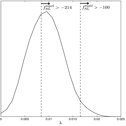
Figure 2: One-dimensional marginalized probability distribution of the parameter $\lambda$ in the dilatonic ghost condensate model constrained by the joint data analysis of WMAP 7yr, BAO, and HST. We also show the bound on $\lambda$ coming from the WMAP 7yr constraint of the equilateral non-Gaussianity parameter, $f_{\rm NL}^{\rm equil}>-214$, as well as the bound on $\lambda$ corresponding to the constraint $f_{\rm NL}^{\rm equil}>-100$.

IV.4 DBI field

The DBI field $\phi$ is characterized by the Lagrangian

$$P=-f(\phi)^{-1}\sqrt{1-2f(\phi)X}+f(\phi)^{-1}-V(\phi)\,,$$ (63)

where $f(\phi)$ and $V(\phi)$ are functions of $\phi$. If we choose

$$g(Y)=-\sqrt{1-2Y}/Y-c/Y\,,$$ (64)

the Lagrangian $P=Xg(Y)$ reduces to (63) with $f(\phi)=e^{\lambda\phi}$ and $V(\phi)=(c+1)e^{-\lambda\phi}$. Hence the DBI field with the exponential potential $V(\phi)=(c+1)e^{-\lambda\phi}$ leads to assisted inflation.

For the function (64) it follows that

$$\epsilon=\frac{3Y}{c\sqrt{1-2Y}+1}\,,\quad c_{s}^{2}=1-2Y\,.$$ (65)

If $c\lesssim 1$, one has $\epsilon\ll 1$ and $c_{s}^{2}\simeq 1$ for $Y\ll 1$. This case is similar to tachyon inflation in which cosmic acceleration is driven by the field potential. One can also realize $\epsilon\ll 1$ under the following condition

$$c\sqrt{1-2Y}\gg 1\,.$$ (66)

If $c\gg 1$, then it is possible to satisfy (66) even for the values of $Y$ close to 1/2. In fact this is the ultra-relativistic regime of the DBI inflation in which the $\gamma$ factor $\gamma=1/\sqrt{1-f(\phi)\dot{\phi}^{2}}$ is much larger than 1. Even in this “fast-roll” regime the presence of the potential is important to satisfy the condition (66).

The inflationary observables are

$$n_{\rm s}-1 = n_{\rm t}=-\frac{3(1-c_{s}^{2})}{c\,c_{s}+1}\,,$$ (67)

$$r = \frac{24c_{s}(1-c_{s}^{2})}{c\,c_{s}+1}\,,$$ (68)

$$f_{\rm NL}^{\rm equil} = -\frac{55}{1944}\frac{(10c\,c_{s}-71)}{(c\,c_{s}+1)}\left(\frac{1}{c_{s}^{2}}-1\right)\,,$$ (69)

where $c_{s}=\sqrt{1-2Y}$. These observables depend not only on $c_{s}$ (or $Y$) but on the coefficient $c$ associated with the field potential. For larger $c$ it is possible to satisfy the observational constraints of $n_{\rm s}$, $r$, and $n_{\rm t}$ with smaller $c_{s}$, because the denominators of Eqs. (67) and (68) get larger. In fact, Fig. 3 shows that, for larger $c$, the one-dimensional marginalized probability distribution of $\lambda$ tends to shift to the regions of smaller $c_{s}$. In Fig. 3 the propagation speed $c_{s}$ close to 1 is not favored because $n_{\rm s}$ and $r$ are close to the HZ spectrum. The models with very small $c_{s}$ are also disfavored because of the large deviation from the HZ spectrum.

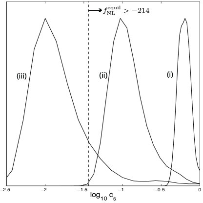
Figure 3: One-dimensional marginalized probability distribution of the field propagation speed $c_{s}$ (with the logarithmic scale) in the DBI model constrained by the observational data of WMAP 7yr, BAO, and HST. The three solid lines correspond to the cases: (i) $c=10^{2}$, (ii) $c=10^{3}$, and (iii) $c=10^{4}$. We also show the bound derived from the non-Gaussianity constraint $f_{\rm NL}^{\rm equil}>-214$ in the limit $cc_{s}\gg 1$.

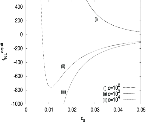
Figure 4: The equilateral non-Gaussianity parameter $f_{\rm NL}^{\rm equil}$ versus the scalar propagation speed $c_{s}$ in the DBI model for (i) $c=10^{2}$, (ii) $c=10^{3}$, and (iii) $c=10^{4}$. For $c=10^{2}$ the scalar propagation speed is constrained by the WMAP 7yr upper bound $f_{\rm NL}^{\rm equil}<266$, whereas for $c=10^{3}$ and $c=10^{4}$ it is constrained by the lower bound $f_{\rm NL}^{\rm equil}>-214$.

In Fig. 4 we plot the non-Gaussianity parameter $f_{\rm NL}^{\rm equil}$ given in Eq. (69) versus the scalar propagation speed $c_{s}$ for three different values of $c$. For $c=10^{2}$ we obtain the bound $c_{s}>3.2\times 10^{-2}$ from the WMAP 7yr upper limit $f_{\rm NL}^{\rm equil}<266$. On the other hand, the WMAP 7yr lower limit $f_{\rm NL}^{\rm equil}>-214$ gives the bounds $c_{s}>3.1\times 10^{-2}$ and $c_{s}>3.6\times 10^{-2}$ for $c=10^{3}$ and $c=10^{4}$, respectively.

As we see in Fig. 3, the CMB likelihood analysis in terms of $n_{\rm s}$, $r$, and $n_{\rm t}$ places the constraints on $c_{s}$, as $0.48<c_{s}<0.84$ (95 % CL) for $c=10^{2}$ and $0.06<c_{s}<0.35$ (95 % CL) for $c=10^{3}$. If $c\lesssim 10^{3}$ the non-Gaussianity does not provide additional constraints on $c_{s}$ to those derived by the likelihood analysis in Fig. 3. If $c\gtrsim 10^{3}$ the non-Gaussianity plays an important role to restrict the allowed parameter space of $c_{s}$ further. In particular, for $c=10^{4}$, there are almost no allowed regions to satisfy all the observational constraints (see Fig. 3). Hence the models with $c\gtrsim 10^{4}$ are excluded by the analysis including non-Gaussianities.

V More general models

So far we have studied the observational constraints on four assisted inflation models. Among them the dilatonic ghost condensate and the DBI models can be tightly constrained by taking into account the bound coming from the primordial non-Gaussianity. This is associated with the fact that both $\epsilon$ and $c_{s}^{2}$ can be much smaller than 1 in those models. In this section we shall extend the analysis to more general functions of $g(Y)$.

In the dilatonic ghost condensate model the numerators of $\epsilon$ and $c_{s}^{2}$ in Eq. (57) vanish at $cY=1/2$, whereas the denominators of them are non-zero finite values. In the DBI model the numerator of $\epsilon$ in Eq. (65) does not vanish in the ultra-relativistic regime ($Y\approx 1/2$), whereas $c_{s}^{2}\ll 1$. In the DBI case it is possible to have $\epsilon\ll 1$ as long as the denominator of $\epsilon$ is much larger than the numerator of it [which is satisfied under the condition (66)]. Since these models are qualitatively different, we classify the assisted k-inflation models into two classes in the following discussion.

V.1 Class (i)

Let us first study the models in which inflation occurs around $Y=Y_{0}$, where $Y_{0}$ satisfies

$$g(Y_{0})+Y_{0}g^{\prime}(Y_{0})=0\,.$$ (70)

As in the case of the dilatonic ghost condensate, we consider the models in which the numerators of $\epsilon$ and $c_{s}^{2}$ in Eqs. (41) and (42) vanish, whereas the denominators are non-zero. Since $Y=Y_{0}$ corresponds to the exact de Sitter solution, we perform the linear expansion of the variables $\epsilon(Y)$ and $c_{s}^{2}(Y)$ by setting $Y=Y_{0}+\delta Y$ with $|\delta Y/Y_{0}|\ll 1$. It then follows that

$$\epsilon(Y) \simeq \epsilon^{\prime}(Y_{0})\,\delta Y=\frac{6}{Y_{0}}\left[1+\frac{Y_{0}g^{\prime\prime}(Y_{0})}{2g^{\prime}(Y_{0})}\right]\,\delta Y\,,$$ (71)

$$c_{s}^{2}(Y) \simeq {c_{s}^{2}}^{\prime}(Y_{0})\,\delta Y=\frac{1}{2Y_{0}}\,\delta Y\,.$$ (72)

This shows that the ratio $c_{s}^{2}/\epsilon$ is approximately constant in the regime $|\delta Y/Y_{0}|\ll 1$:

$$\frac{c_{s}^{2}}{\epsilon}\simeq\frac{1}{12}\left[1+\frac{Y_{0}g^{\prime\prime}(Y_{0})}{2g^{\prime}(Y_{0})}\right]^{-1}\,.$$ (73)

Expanding Eq. (40) at $Y=Y_{0}$, we have

$$(\delta Y)^{2}=\frac{Y_{0}g^{\prime}(Y_{0})}{6[2g^{\prime}(Y_{0})+Y_{0}g^{\prime\prime}(Y_{0})]^{2}}\lambda^{2}\,.$$ (74)

As long as $g^{\prime}(Y_{0})>0$ there exists a solution with $\delta Y>0$. The conditions (29) for the avoidance of ghosts and Laplacian instabilities translate into

$$g^{\prime}(Y_{0}) > 0\,,$$ (75)

$$Y_{0}g^{\prime\prime}(Y_{0}) > -2g^{\prime}(Y_{0})\,.$$ (76)

In the ghost condensate model described by the function $g(Y)=-1+cY$ the second derivative $g^{\prime\prime}(Y)$ automatically vanishes, which gives $c_{s}^{2}/\epsilon=1/12$. In this model the variable $\lambda$ is observationally bounded as $\lambda<1.5\times 10^{-2}$ (95 % CL), in which case $\delta Y/Y_{0}=\lambda/(2\sqrt{3})<4.3\times 10^{-3}$. Hence it is a good approximation to use the linear expansion given above. In fact we have carried out the CMB likelihood analysis by employing the relation $c_{s}^{2}/\epsilon=1/12$ and confirmed that the observational bound on $\lambda$ is very similar to that given in Eq. (62).

We study the following more general models

$$g(Y)=c_{0}+\sum_{p\neq 0}c_{p}Y^{p}\,,$$ (77)

where $c_{p}$ are constants. The power $p$ can be integer or some real number. From Eq. (73) the ratio $c_{s}^{2}/\epsilon$ is given by

$$\frac{c_{s}^{2}}{\epsilon}\simeq\frac{1}{6}\frac{\sum pc_{p}Y_{0}^{p-1}}{\sum p(p+1)c_{p}Y_{0}^{p-1}}\,.$$ (78)

For the single power $p$, i.e. $g(Y)=c_{0}+c_{p}Y^{p}$, Eq. (78) reduces to

$$\frac{c_{s}^{2}}{\epsilon}\simeq\frac{1}{6(p+1)}\,.$$ (79)

The conditions (75) and (76) give $pc_{p}>0$ and $p(p+1)c_{p}>0$, respectively, which demand that $p>-1$. More precisely we require $c_{p}<0$ for $-1<p<0$ and $c_{p}>0$ for $p>0$. In Fig. 5 we plot the line (79) in the $(\epsilon,c_{s}^{2})$ plane for five different values of $p$ ($=-0.5,0.5,1,2,3$). The ghost condensate model corresponds to $p=1$ with the tangent $c_{s}^{2}/\epsilon=1/12$.

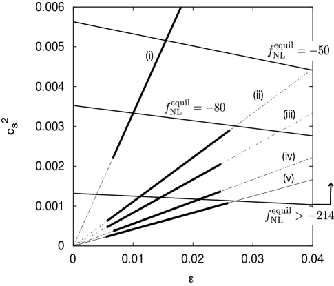
Figure 5: The thin lines show the relations between $\epsilon$ and $c_{s}^{2}$ for the models $g(Y)=c_{0}+c_{p}Y^{p}$ with (i) $p=-0.5$, (ii) $p=0.5$, (iii) $p=1$, (iv) $p=2$, and (v) $p=3$, in the regime $\epsilon\ll 1$. The bold lines correspond to the observational constraints (95 % CL) on each model derived from the joint data analysis of WMAP 7yr, BAO, and HST. We also plot the boundary coming from $f_{\rm NL}^{\rm equil}>-214$ as well as the curves corresponding to $f_{\rm NL}^{\rm equil}=-50$ and $f_{\rm NL}^{\rm equil}=-80$.

We carry out the CMB likelihood analysis for the models $g(Y)=c_{0}+c_{p}Y^{p}$ with $p=-0.5,0.5,1,2,3$ by employing the linear expansion given above. The observational constraints shown in Fig. 5 with the bold lines are derived by using the theoretical values of $n_{\rm s}$, $r$, and $n_{\rm t}$ given in Eqs. (43) and (44) with the relation (79). In the $(\epsilon,c_{s}^{2})$ plane we also plot the border corresponding to the WMAP 7yr lower bound $f_{\rm NL}^{\rm equil}=-214$. The region above this border satisfies the observational constraint of the non-Gaussianity. From Fig. 5 we find that there is no viable parameter space for $p\geq 3$ satisfying all the observational constraints. As long as the bold lines plotted in Fig. 5 are above the border corresponding to $f_{\rm NL}^{\rm equil}=-214$, the models with $p<3$ can be compatible with the observational data. If the future observations can place the bound on $f_{\rm NL}^{\rm equil}$ larger than $-80$, the models with $p>1/2$ can be ruled out (see Fig. 5).

Let us also discuss the case in which the function $g(Y)$ is the sum of different powers of $p$. For example we consider the model

$$g(Y)=c_{0}+c_{1}Y+c_{-1}Y^{-1}\,.$$ (80)

This corresponds to the dilatonic ghost condensate in the presence of the exponential potential, i.e. $P=c_{0}X+c_{1}e^{\lambda\phi}X^{2}+c_{-1}e^{-\lambda\phi}$. Substituting Eq. (80) into Eq. (70), we obtain $Y_{0}=-c_{0}/(2c_{1})$. The conditions (75) and (76) translate into $c_{1}(1-4c_{1}c_{-1}/c_{0}^{2})>0$ and $c_{1}>0$, respectively. Since $Y_{0}=-c_{0}/(2c_{1})>0$, we require that

$$c_{0}<0\,,\quad c_{1}>0\,,\quad 4c_{1}c_{-1}/c_{0}^{2}<1\,.$$ (81)

From Eq. (78) we have

$$\frac{c_{s}^{2}}{\epsilon}=\frac{1}{12}\left(1-\frac{4c_{1}c_{-1}}{c_{0}^{2}}\right)\,.$$ (82)

If $c_{-1}>0$, then the tangent of the line (82) gets smaller relative to that in the ghost condensate model. Figure 5 shows that the allowed parameter space tends to be narrower for smaller $c_{s}^{2}/\epsilon$. The existence of a viable parameter demands the following condition

$$\frac{c_{1}c_{-1}}{c_{0}^{2}}\lesssim 0.1\,.$$ (83)

The effect of the negative exponential potential $V=-c_{-1}e^{-\lambda\phi}$ (with $c_{-1}>0$) needs to be suppressed to be consistent with the bound (83). In contrast, the tangent of the line (82) gets larger than $1/12$ when $c_{-1}<0$. The effect of the positive exponential potential $V=-c_{-1}e^{-\lambda\phi}$ (with $c_{-1}<0$) makes it easier to satisfy the observational constraints.

V.2 Class (ii)

In the DBI model, inflation occurs in the ultra-relativistic regime ($Y\approx 1/2$) under the condition (66). In this case the denominator of $\epsilon$ in Eq. (65) is much larger than its numerator. Since the linear expansion around $Y=1/2$ is not possible in such cases, we need to treat this class of models separately. Let us take the function of the form

$$g(Y)=-\frac{c}{Y}\left[1+f(Y)\right]\,,$$ (84)

in which case Eqs. (41) and (42) give

$$\epsilon=-\frac{3Yf^{\prime}(Y)}{1+f(Y)-2Yf^{\prime}(Y)}\,,$$ (85)

$$c_{s}^{2}=\frac{f^{\prime}(Y)}{f^{\prime}(Y)+2Yf^{\prime\prime}(Y)}\,.$$ (86)

In the DBI model with $f(Y)=\sqrt{1-2Y}/c$, we can realize inflation in the regime $|f^{\prime}(Y)|=1/[|c|\sqrt{1-2Y}]\ll 1$ and $f(Y)\ll 1$ with $Y\approx 1/2$, so that $\epsilon\ll 1$.

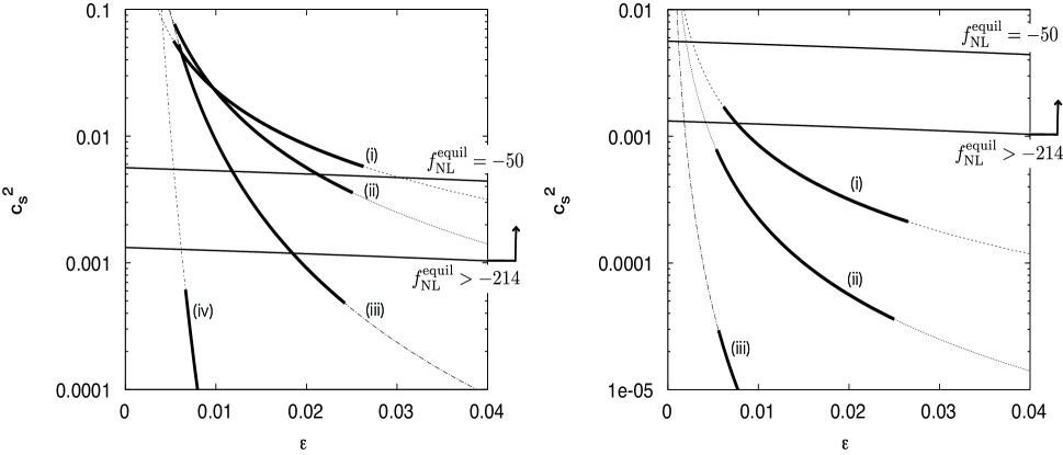
Figure 6: The thin curves show the relation between $\epsilon$ and $c_{s}^{2}$ for the models (84) with (87). The left and right panels correspond to $c=10^{3}$ and $c=10^{4}$, respectively, with (i) $m=0.3$, (ii) $m=0.5$, (iii) $m=0.7$, and (iv) $m=0.9$. The bold curves represent the observational constraints (95 % CL) derived from the CMB likelihood analysis in terms of $n_{\rm s}$, $r$, and $n_{\rm t}$. We also plot the borders corresponding to the WMAP 7yr bound $f_{\rm NL}^{\rm equil}>-214$ as well as $f_{\rm NL}^{\rm equil}=-50$.

We study the models (84) with

$$f(Y)=(1-2Y)^{m}/c\,.$$ (87)

From Eqs. (85) and (86) we have

$$\epsilon=\frac{6mY}{c(1-2Y)^{1-m}+1+2(2m-1)Y}\,,$$ (88)

$$c_{s}^{2}=\frac{1-2Y}{1-2(2m-1)Y}\,.$$ (89)

We consider the case in which inflation occurs for the values of $Y$ slightly smaller than $1/2$, while satisfying the condition $c(1-2Y)^{1-m}\gg 1$. Since we require $\epsilon\simeq 3m/[c(1-2Y)^{1-m}]>0$ and $c_{s}^{2}\simeq(1-2Y)/[2(1-m)]>0$, we have either $0<m<1$ with $c>0$ or $m<0$ with $c<0$. The following relation also holds between $c_{s}$ and $\epsilon$:

$$c_{s}^{2(1-m)}\simeq\frac{3m}{c[2(1-m)]^{1-m}}\frac{1}{\epsilon}\,.$$ (90)

In Fig. 6 we plot the curve (90) in the $(\epsilon,c_{s}^{2})$ plane for four different values of $m$ ($=0.3,0.5,0.7,0.9$). The left and right panels correspond to the cases $c=10^{3}$ and $c=10^{4}$, respectively. We also show the observational bounds constrained by $n_{\rm s}$, $r$, and $n_{\rm t}$ (plotted as the bold lines) as well as the curves corresponding to $f_{\rm NL}^{\rm equil}=-214$ and $f_{\rm NL}^{\rm equil}=-50$.

When $c=10^{3}$ there exists some allowed parameter space for the models with $m\leq 0.7$ (including the DBI model with $m=0.5$), but for $m\geq 0.9$ the WMAP 7yr bound of the non-Gaussianity excludes the parameter region constrained by the linear perturbations. For larger $c$ the theoretical curves in Fig. 6 shift to the regions with smaller $c_{s}$, so that the constraint from the non-Gaussianity tends to be more important. For $c=10^{4}$ the right panel of Fig. 6 shows that, the models with $m\geq 0.5$ do not have the viable parameter space satisfying all the current observational constraints. If the future observations can reach the level of the lower limit of the non-Gaussianity with $|f_{\rm NL}^{\rm equil}|={\cal O}(10)$, then it is possible to place tighter constraints further (see the curves in Fig. 6 corresponding to $f_{\rm NL}^{\rm equil}=-50$).

VI Conclusions

We have studied the observational constraints on assisted k-inflation models in which the multiple scalar fields join an effective single-field attractor described by the Lagrangian $P=Xg(Y)$ with $Y=Xe^{\lambda\phi}$. The canonical field with the exponential potential, $P=X-ce^{-\lambda\phi}$ (i.e. $g(Y)=1-c/Y$), is one of the simplest examples giving rise to assisted inflation. The effective slope $\lambda$ along the inflationary attractor is given by $\lambda=\left(\sum_{i=1}1/\lambda_{i}^{2}\right)^{-1/2}$, which is smaller than the slopes $\lambda_{i}$ for each exponential potential. The same structure holds for the k-inflation models with the Lagrangian $P=Xg(Y)$ for arbitrary functions of $g(Y)$.

Along the effective single-field attractor, the inflationary observables are in general given by Eqs. (43)-(45). In Sec. IV we have confronted four models of assisted inflation with the recent observations of CMB combined with BAO and HST. For the canonical field with the exponential potential the effective slope $\lambda$ is constrained to be $0.086<\lambda<0.228$. The tachyon field needs to have a small kinetic energy relative to its potential energy for the realization of inflation, in which case the observational bound on the variable $Y$ is given by Eq. (55). Since the field propagation speed $c_{s}$ is close to 1 in this case, the primordial non-Gaussianity remains to be small for the tachyon model.

In the dilatonic ghost condensate model the non-Gaussianity provides additional constraints to those derived by the spectra of scalar and tensor perturbations. As we see in Fig. 2, the WMAP 7 yr limit $f_{\rm NL}^{\rm equil}>-214$ reduces the allowed parameter space of the parameter $\lambda$. If the lower bound on $f_{\rm NL}^{\rm equil}$ reaches the level of $-100$ in future observations, it will be possible to rule out the dilatonic ghost condensate model. In the DBI model the level of the non-Gaussianity depends on the field propagation speed $c_{s}$ as well as the constant $c$ associated with the energy scale of the potential. For larger $c$, $|f_{\rm NL}^{\rm equil}|$ tends to increase, so that the models can be constrained by the additional information coming from the non-Gaussianity. In fact the DBI model with $c\gtrsim 10^{4}$ is excluded by the WMAP 7yr data.

We have extended the analysis to more general functions $g(Y)$ by classifying the assisted k-inflation models into two classes. The first class consists of the models in which inflation occurs around $Y=Y_{0}$ satisfying the condition $g(Y_{0})+Y_{0}g^{\prime}(Y_{0})=0$. The representative models of this class are $g(Y)=c_{0}+\sum_{p\neq 0}c_{p}Y^{p}$, which includes the dilatonic ghost condensate. From the CMB likelihood analysis combined with the non-Gaussianity bound we have found that the single-power models $g(Y)=c_{0}+c_{p}Y^{p}$ with $p\geq 3$ are ruled out. The second class consists of the models with the speed limit of the field, which includes the DBI model as a specific case. We have carried out the CMB likelihood analysis for the functions $g(Y)=-(c/Y)[1+(1-2Y)^{m}/c]$ ($m<1$) and showed that the models with larger $m$ and $c$ tend to be observationally disfavored by taking into account the non-Gaussianity bound.

In this paper we have evaluated the inflationary observables under the assumption that the solutions are on the assisted attractor described by the effective single field. In order to end inflation the solutions need to exit from this regime. This can be achieved by treating the validity of our Lagrangian $P=Xg(Y)$ only within some limited range of field values. With some suitable modification of the Lagrangian it is possible to lead to the graceful exit of inflation kinflation . Another possibility is that k-inflation ends with a phase transition as in hybrid inflation Arkani2 . It will be also of interest to study the case where the observed CMB anisotropies correspond to the epoch before the multiple fields join the inflationary attractor. In this case the trajectory in field space is curved, so that isocurvature perturbations can contribute to adiabatic perturbations Bruce . We leave these issues for future work.

References

- (1) A. A. Starobinsky, Phys. Lett. B 91 (1980) 99; D. Kazanas, Astrophys. J. 241 L59 (1980); K. Sato, Mon. Not. R. Astron. Soc. 195, 467 (1981); A. H. Guth, Phys. Rev. D 23, 347 (1981).
- (2) V. F. Mukhanov and G. V. Chibisov, JETP Lett. 33, 532 (1981); A. H. Guth and S. Y. Pi, Phys. Rev. Lett. 49 (1982) 1110; S. W. Hawking, Phys. Lett. B 115, 295 (1982); A. A. Starobinsky, Phys. Lett. B 117 (1982) 175.
- (3) J. E. Lidsey et al., Rev. Mod. Phys. 69, 373 (1997).
- (4) D. H. Lyth and A. Riotto, Phys. Rept. 314, 1 (1999).
- (5) B. A. Bassett, S. Tsujikawa and D. Wands, Rev. Mod. Phys. 78, 537 (2006).
- (6) G. F. Smoot et al., Astrophys. J. 396, L1-L5 (1992).
- (7) E. Komatsu et al. [WMAP Collaboration], Astrophys. J. Suppl. 192, 18 (2011).
- (8) [PLANCK Collaboration], arXiv:astro-ph/0604069.
- (9) N. Bartolo, S. Matarrese, A. Riotto, Phys. Rev. D65, 103505 (2002); V. Acquaviva, N. Bartolo, S. Matarrese and A. Riotto, Nucl. Phys. B667, 119-148 (2003); N. Bartolo, E. Komatsu, S. Matarrese and A. Riotto, Phys. Rept. 402, 103-266 (2004).
- (10) J. M. Maldacena, JHEP 0305, 013 (2003).
- (11) D. H. Lyth and Y. Rodriguez, Phys. Rev. Lett. 95, 121302 (2005); D. H. Lyth and Y. Rodriguez, Phys. Rev. D 71, 123508 (2005); D. H. Lyth, K. A. Malik and M. Sasaki, JCAP 0505, 004 (2005).
- (12) D. S. Salopek and J. R. Bond, Phys. Rev. D 42, 3936 (1990); A. Gangui, F. Lucchin, S. Matarrese and S. Mollerach, Astrophys. J. 430, 447 (1994); E. Komatsu and D. N. Spergel, Phys. Rev. D63, 063002 (2001).
- (13) C. Armendariz-Picon, T. Damour and V. F. Mukhanov, Phys. Lett. B 458, 209 (1999).
- (14) D. Seery and J. E. Lidsey, JCAP 0506, 003 (2005).
- (15) X. Chen, M. x. Huang, S. Kachru and G. Shiu, JCAP 0701, 002 (2007); X. Chen, R. Easther and E. A. Lim, JCAP 0706, 023 (2007); JCAP 0804, 010 (2008).
- (16) J. Garriga and V. F. Mukhanov, Phys. Lett. B 458, 219 (1999).
- (17) J. c. Hwang and H. Noh, Phys. Rev. D 66, 084009 (2002).
- (18) A. De Felice and S. Tsujikawa, arXiv:1103.1172 [astro-ph.CO].
- (19) A. R. Liddle, A. Mazumdar and F. E. Schunck, Phys. Rev. D 58, 061301 (1998).
- (20) K. A. Malik and D. Wands, Phys. Rev. D 59, 123501 (1999); E. J. Copeland, A. Mazumdar and N. J. Nunes, Phys. Rev. D 60, 083506 (1999); P. Kanti and K. A. Olive, Phys. Lett. B 464, 192 (1999); A. M. Green and J. E. Lidsey, Phys. Rev. D 61, 067301 (2000); A. Mazumdar, S. Panda and A. Perez-Lorenzana, Nucl. Phys. B 614, 101 (2001); M. C. Bento, O. Bertolami and N. M. C. Santos, Phys. Rev. D 65, 067301 (2002); A. Collinucci, M. Nielsen and T. Van Riet, Class. Quant. Grav. 22, 1269 (2005); S. A. Kim, A. R. Liddle and S. Tsujikawa, Phys. Rev. D 72, 043506 (2005); J. Hartong, A. Ploegh, T. Van Riet and D. B. Westra, Class. Quant. Grav. 23, 4593 (2006).
- (21) P. G. Ferreira and M. Joyce, Phys. Rev. Lett. 79, 4740 (1997); Phys. Rev. D 58, 023503 (1998).
- (22) E. J. Copeland, A. R. Liddle and D. Wands, Phys. Rev. D 57, 4686 (1998).
- (23) F. Piazza and S. Tsujikawa, JCAP 0407, 004 (2004).
- (24) S. Tsujikawa and M. Sami, Phys. Lett. B 603, 113 (2004).
- (25) S. Tsujikawa, Phys. Rev. D 73, 103504 (2006).
- (26) L. Amendola, M. Quartin, S. Tsujikawa and I. Waga, Phys. Rev. D 74, 023525 (2006).
- (27) J. J. Halliwell, Phys. Lett. B 185, 341 (1987); F. Lucchin and S. Matarrese, Phys. Rev. D 32, 1316 (1985); J. Yokoyama and K. i. Maeda, Phys. Lett. B 207, 31 (1988); A. B. Burd and J. D. Barrow, Nucl. Phys. B 308, 929 (1988).
- (28) N. Arkani-Hamed, H. C. Cheng, M. A. Luty and S. Mukohyama, JHEP 0405, 074 (2004).
- (29) N. Arkani-Hamed, P. Creminelli, S. Mukohyama and M. Zaldarriaga, JCAP 0404, 001 (2004).
- (30) J. Ohashi and S. Tsujikawa, Phys. Rev. D 80, 103513 (2009).
- (31) W. Percival et al., Mon. Not. Roy. Astron. Soc. 1741 (2009).
- (32) A. G. Riess et al., Astrophys. J. 699, 539 (2009).
- (33) A. Sen, JHEP 0204, 048 (2002); M. Fairbairn, M. H. G. Tytgat, Phys. Lett. B546, 1-7 (2002); M. Sami, P. Chingangbam, T. Qureshi, Phys. Rev. D66, 043530 (2002).
- (34) E. Silverstein and D. Tong, Phys. Rev. D 70, 103505 (2004); M. Alishahiha, E. Silverstein and D. Tong, Phys. Rev. D 70, 123505 (2004).
- (35) R. L. Arnowitt, S. Deser, C. W. Misner, Phys. Rev. 117, 1595-1602 (1960).
- (36) P. Creminelli et al., JCAP 0605, 004 (2006).
- (37) K. Koyama, Class. Quant. Grav. 27, 124001 (2010).
- (38) http://cosmologist.info/cosmomc/
- (39) A. Feinstein, Phys. Rev. D66, 063511 (2002); T. Padmanabhan, Phys. Rev. D66, 021301 (2002); E. J. Copeland, M. R. Garousi, M. Sami, S. Tsujikawa, Phys. Rev. D71, 043003 (2005).
- (40) C. Gordon, D. Wands, B. A. Bassett, R. Maartens, Phys. Rev. D63, 023506 (2001); N. Bartolo, S. Matarrese, A. Riotto, Phys. Rev. D64, 123504 (2001); S. Tsujikawa, D. Parkinson, B. A. Bassett, Phys. Rev. D67, 083516 (2003).