Exciton dynamics and Quantumness of energy transfer in the Fenna-Matthews-Olson complex

Abstract

We present numerically exact results for the quantum coherent energy transfer in the Fenna-Matthews-Olson molecular aggregate under realistic physiological conditions, including vibrational fluctuations of the protein and the pigments for an experimentally determined fluctuation spectrum. We find coherence times shorter than observed experimentally. Furthermore we determine the energy transfer current and quantify its “quantumness” as the distance of the density matrix to the classical pointer states for the energy current operator. Most importantly, we find that the energy transfer happens through a “Schrödinger-cat” like superposition of energy current pointer states.

I Introduction

Recent experiments on the ultrafast exciton dynamics in photosynthetic biomolecules have brought a longstanding question again into the scientific focus whether nontrivial quantum coherence effects exist in natural biological systems under physiological conditions, and, if so, whether they have any functional significance. Photosynthesis vanAmerongen00 starts with the harvest of a photon by a pigment and the formation of an exciton, followed by its transfer to the reaction center, where charge separation via a primary electron transfer is initiated. The transfer of excitations has traditionally been regarded as an incoherent hopping between molecular sites MayKuehn .

Recently, Engel et al. EngelFleming07 ; Engel10 have reported longlasting beating signals in time-resolved optical two-dimensional spectra of the Fenna-Matthews-Olson (FMO) Fenna75 ; Milder10 complex, which have been interpreted as evidence for quantum coherent energy transfer via delocalized exciton states. It transfers the excitonic energy from the chlorosome to the reaction center and consists of three identical subunits, each with seven bacteriochlorophyll molecular sites (the existence of an eighth site is presently under investigation). Quantum coherence times of more than 660 fs at $77$ K EngelFleming07 and about $300$ fs at physiological temperatures Engel10 have been reported.

Together with recent experiments Scholes10 on marine cryptophyte algae, these reports have boosted on-going research to answer the question how quantum coherence can prevail over such long times in a strongly fluctuating physiological environment of strong vibronic protein modes and the surrounding polar solvent. Theoretical modeling of the real-time dynamics is notoriously complicated due to the large cluster size and strong non-Markovian fluctuations. It relies on simple models Reineker82 of few chromophore sites which interact by dipolar couplings and which are exposed to fluctuations of the solvent and the protein vanAmerongen00 ; MayKuehn . A calculation of the 2D optical spectrum assuming weak coupling to the environment does not reproduce the experimental data Sharp10 . It also became clear that standard Redfield-type approaches fail even for dimers Ishizaki09a ; Nalbach10a .

In connection with molecular exciton transfer, extensions beyond perturbative approaches, such as the stochastic Liouville equation Reineker82 , extended Lindblad approaches Mukamel2009 or small polaron approaches Jang08 , have been formulated. Two recent approaches have included parts of the standard FMO model. A second-order cumulant time-nonlocal quantum master equation found coherence times AkiPNAS09 as observed experimentally for the FMO complex. However, they employed an Ohmic bath in which the relaxation time is not uniquely fixed by experiments and excluding strong vibrational protein modes. On the other hand, a variant of a time-dependent DMRG scheme Plenio10 has been applied to a dimer in a realistic FMO environment Adolphs06 . The solution of the full state-of-the-art FMO model with seven localized sites and a physical environmental spectrum Adolphs06 including a strongly localized Huang-Rhys mode MayKuehn is still missing. In particular, it has not been clarified whether a strong vibronic mode still allows for the observed quantum coherence times.

In this paper we close this gap and present numerically exact results for the full FMO model with seven sites and the spectral density of Ref. Adolphs06 , determined from optical spectra Pullerits00 . Upon adopting the iterative real-time quasiadiabatic propagator path-integral (QUAPI) Makri95a ; Thorwart98 scheme we find coherence times shorter than observed experimentally. For comparisson we recalculate also the dynamics employing the same Ohmic fluctuation spectrum as Ishizaki and Fleming AkiPNAS09 . To quantify quantum effects for energy transfer, we calculate the energy current associated with the transfer dynamics and its “quantumness”. It has been argued that quantum entanglement could be created in a single excitation sub-space during the energy transfer Whaley , but this form of entanglement cannot be used to violate a Bell-inequality Beenakker06 and its role for the transfer efficiency is therefore unclear. Wilde et al. Wilde used the Leggett-Garg inequality to discuss whether quantum effects are relevant but they applied a phenomenological Lindblad approach. Here we use a recently developed measure of quantumness based on the Hilbert-Schmidt distance of the density matrix to the convex hull of classical states Giraud10 , taken as the “pointer-states” Zurek81 of the energy-current operator. We show that energy transfer starts with large current out of the initial site and then small currents flow between all seven sites. All currents show substantial quantumness. Interestingly enough, this implies that the energy transfer happens through a largely coherent “Schrödinger-cat” like superposition of pointer states of the energy current operator.

In the next section we shortly recapitulate the Hamiltonian and the fluctuation spectrum of the site energies for the Fenna-Matthews-Olson complex. Then we determine the population dynamics within the single excitation subspace. In the fourth section we calculate the energy currents between any two sites in the FMO and then introduce a measure for the quantumness of these currents. Finally we conclude with a short summary of our results.

II FMO Model

The FMO complex is a trimer consisting of identical, weakly interacting monomers Adolphs06 , each containing seven bacteriochlorophylla (BChla) molecular sites which transfer excitons. The pigments are embedded in a large protein complex. Each of it can be reduced to its two lowest electronic levels and their excited states are electronically coupled along the complex. Recombination is negligibly slow ($\sim$ ns) compared to exciton transfer times ($\sim$ps). Thus, the excitation dynamics is reliably described within the 1-exciton subspace. The coupling of the seven excited levels gives rise to the Hamiltonian

$$H_{\rm FMO}=\\ {\footnotesize\left(\begin{array}[]{ccccccc}240&-87.7&5.5&-5.9&6.7&-13.7&-9.9\\ &315&30.8&8.2&0.7&11.8&4.3\\ &&0&-53.5&-2.2&-9.6&6.0\\ &&&130&-70.7&-17.0&-63.3\\ &&&&285&81.1&-1.3\\ &&&&&435&39.7\\ &&&&&&245\end{array}\right)}$$ (1)

in units of cm^-1 in site representation Adolphs06 for an FMO monomer of C. tepidum. We define the lowest site energy of pigment $3$ as reference.

The vibrations of the BChla, the embedding protein and the surrounding polar solvent are too complex for a pure microscopic description and are thus treated with the framework of open quantum systems. They induce thermal fluctuations described by harmonic modes MayKuehn and lead to the total Hamiltonian Adolphs06

$$H = H_{\rm FMO}$$

$$+\sum_{j=1}^{7}|j\rangle\langle j|\sum_{\kappa}\nu_{\kappa}^{(j)}q_{j,{\kappa}}\,+\sum_{j=1}^{7}\mbox{$\frac{1}{2}$}\sum_{\kappa}\left(p_{j,{\kappa}}^{2}+\omega_{j,{\kappa}}^{2}q_{j,{\kappa}}^{2}\right)$$

with momenta $p_{j,{\kappa}}$, displacement $q_{j,{\kappa}}$, frequency $\omega_{j,{\kappa}}$ and coupling $\nu_{\kappa}^{(j)}$ of the environmental vibrations at site $j$. We assume that fluctuations at different sites are identical but spatially uncorrelated Kleinekathoefer10c .

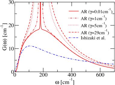
Figure 1: (Color online) Bath spectral densities of the FMO complex of C. tepidum: The most realistic form as determined up to present Adolphs06 ; Pullerits00 is given by Eq. (3) (AR, red (upper four) lines). The blue dash-dot-dashed (lower) line shows the Drude form $G_{D}(\omega)$ used in AkiPNAS09 .

The key quantity which determines the FMO coherence properties is the environmental spectral density $G(\omega)=\sum_{j,\kappa}(|\nu_{\kappa}^{(j)}|^{2}/2\omega_{j,{\kappa}})\delta(\omega-\omega_{j,{\kappa}})$. The most detailed identification of the bath properties up to date has been achieved by Adolphs and Renger Adolphs06 . They used an advanced theory of optical spectra, a genetic algorithm, and excitonic couplings from electrostatic calculations modeling the dielectric protein environment to derive the up to present most detailed spectral density

$$G_{AR}(\omega)\,=\,\omega^{2}S_{0}g_{0}(\omega)\,+\omega^{2}S_{H}\delta(\omega-\omega_{H})\,.$$ (3)

Here, $S_{0}=0.5$, $S_{H}=0.22$, $\omega_{H}=180$cm^-1 and

$$g_{0}(\omega)=6.105\cdot 10^{-5}\cdot\frac{\omega^{3}}{\omega_{1}^{4}}e^{-\sqrt{\frac{\omega}{\omega_{1}}}}+3.8156\cdot 10^{-5}\cdot\frac{\omega^{3}}{\omega_{2}^{4}}e^{-\sqrt{\frac{\omega}{\omega_{2}}}}$$

with $\omega_{1}=0.575$ cm^-1 and $\omega_{2}=2$ cm^-1. It includes a broad continuous part (see red (upper four) lines in Fig. 1) which for $\omega\to 0$ behaves as super-Ohmic, $G_{AR}(\omega)\sim\omega^{5}$, and which describes the protein vibrations with the Huang-Rhys factor $S_{0}$. It was determined from temperature-dependent absorption spectra Pullerits00 . In addition, a vibrational mode of the individual pigments with the Huang-Rhys factor $S_{H}$ is included. We have added a broadening to the unphysical $\delta$-peak, which is justified since the protein is embedded in water as a polar solvent which gives rise to an additional weak Ohmic damping of the protein vibrations. We fix its width to $\gamma_{p}=29$ cm^-1 which was found for the lowest energy peak of protein vibrations in the LH2 complex Kleinekathoefer10 .

In order to recover known results for the transfer dynamics of excitations in the Fenna-Matthews-Olson (FMO) complex embedded in an Ohmic bath AkiPNAS09 , we additionally consider the spectral density used in Ref. AkiPNAS09 given by

$$G_{D}(\omega)=\frac{2\lambda\omega\omega_{c}}{\pi(\omega_{c}^{2}+\omega^{2})}$$ (4)

with a Debye cut-off at frequency $\omega_{c}$ (see blue dash-dot-dashed (lowest) line in Fig. 1). It includes the reorganization energy $\lambda=35$ cm^-1 and the environmental timescale $\omega_{c}^{-1}=50$ fs.

III Population dynamics in the FMO

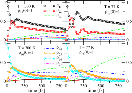
Figure 2: (Color online) Time-dependent occupation probabilities of all seven FMO sites for $T=300$ K, $77$ K with $\rho_{11}(0)=1$ and $\rho_{6}(0)=1$ for the measured FMO spectrum Eq. (3) Adolphs06 .

To understand whether the vibrational fluctuations of the protein and the pigments allow for the observed coherence times, we apply the numerically exact quasi-adiabatic propagator path-integral (QUAPI) to simulate the real time exciton dynamics in the FMO complex for the realistic bath spectral density (3). QUAPI is well established Makri95a ; Thorwart98 and allows us to treat nearly arbitrary spectral functions at finite temperatures. We extended recently the original scheme to treat multiple environments, i.e. separate environments for each chromophore site Nalbach10b .

We calculate the time-dependent populations of the FMO pigment sites for the spectral density of Eq. (3). We choose $T=300$K (physiological temperature) and $T=77$K (typical experimental temperature). Both the pigments BChl $1$ and BChl $6$ are oriented towards the baseplate protein and are thus believed to be initially excited (entrance sites) Wen09 . Thus, we consider two cases, i.e., $\rho_{11}(0)=1$ and $\rho_{66}(0)=1$. We focus on the transient coherence effects and thus do not include an additional sink at the exit site BChl $3$. In Fig. 2, we show the time-dependent pigment occupation probabilities $\rho_{jj}(t)$. Identical simulations using smaller width, i.e. $\gamma_{p}=5$ cm^-1 and $\gamma_{p}=1$ cm^-1, for the vibrational mode yield identical results for the populations (not shown). For $\rho_{66}(0)=1$ at room temperature, coherent oscillations are completely suppressed and at $77$ K they last up to about $250$ fs. For $\rho_{11}(0)=1$, coherence is supported longer due to the strong electronic coupling between sites $1$ and $2$. At room temperature, it survives for up to about $200$ fs and for $77$ K up to $500$ fs at most. Thus, coherence times are shorter than experimentally observed. We emphasize that coherence features are a transient property and, hence, not only the low frequency bath modes, but also the discrete vibrational modes are relevant ($100$ fs corresponds to $\sim 333$ cm^-1).

We additionally calculate the time-dependent populations of the FMO pigment sites for $T=300$K (physiological temperature) and $T=77$K (typical experimental temperature) for the FMO with the bath spectrum $G_{D}(\omega)$ (see Eq. (4)). As above we consider two choices of initial conditions, i.e., $\rho_{11}(0)=1$ and $\rho_{66}(0)=1$ and focus on the transient coherence effects and thus do not include an additional sink at the exit site BChl $3$.

Fig. 3 shows the occupation probabilities of all seven sites at $T=300$ K versus time. For both initial conditions, coherent oscillations of the populations of the initial site and its neighboring site ($j=2$ for $\rho_{11}(0)=1$ and $j=5$ for $\rho_{66}(0)=1$) occur due to the strong electronic couplings. They last up to $\sim 350$ fs. At $T=77$ K, as shown in Fig. 3 (b) and 3(d), the oscillations persist up to $\sim 700$ fs. Our results coincide with those of Ref. AkiPNAS09 . Tiny deviations at short times arise since the full FMO trimer is considered in Ref. AkiPNAS09 . The coherence times, however, are not affected.

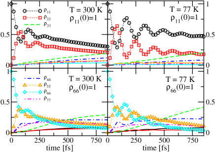
Figure 3: (Color online) Time-dependent occupations of the seven FMO sites for $T=300$ K and $T=77$ K with $\rho_{11}(0)=1$ and $\rho_{66}(0)=1$ for the Ohmic spectrum $G_{D}(\omega)$.

IV Quantumness of Energy transfer through FMO

Next, we discuss whether energy transfer dynamics is a quantum coherent process. Classical coupled dipoles can show oscillatory energy currents identical to quantum mechanical dipole-coupled systems provided that the interaction between the dipoles is weak enough to be treated via linear response Zimanyi . In FMO (see Eq. 1), however, off-diagonal couplings are on the same order of magnitude as site energy differences. We use a physically well motivated measure of quantumness which can be found by first identifying the most classical pure states in the problem. In quantum optics, for instances, coherent states are considered “(most) classical” due to their minimal uncertainty and their stability under the free evolution of the electro-magnetic field Scully97 . Next, one identifies the set of all classical states with the convex hull (i.e. all mixtures) of the pure classical states, as mixing cannot increase quantumness. This leads in quantum optics and for spin-systems to the well established notion that classical states are those with a well-defined positive $P$-function Mandel ; Knight ; Giraud08 ; Giraud10 . Finally, one defines “quantumness” as the distances to the closest classical states.

For FMO we are interested in the “quantumness” of the energy current since energy transfer constitutes the main function of the FMO complex. A measurement of the energy current would yield that for any measurement result the state of the system would collapse onto a pointer state. In general, pointer states are the states einselected by the interaction with its environment Zurek81 being here the hypothetical measurement apparatus for measuring energy current. Pointer states are the most classical states in that they arise via decoherence and are those that persist when a quantum system interacts strongly and for a long time with its environment. In our case of a projective von Neumann measurement, they are the eigenstates of the quantum mechanical operator corresponding to the energy current measurement.

IV.1 Energy currents in FMO

An energy current operator can be derived for a general multi-site Hamiltonian Hardy63 . The expression for an energy current operator ${\bf j}({\bf x})$ can be obtained from a continuity equation

$$\dot{H}({\bf x})+\nabla\cdot{\bf j}({\bf x})=0\,,$$ (5)

where $H({\bf x})$ is the local energy density. This is a well-established procedure introduced by Hardy Hardy63 , and which was largely adopted by a large number of subsequent papers (see e.g. deppe_energy_1994 ; segal_thermal_2003 ; allen_thermal_1993 ; leitner_frequency-resolved_2009 ; wu_energy_2009 .) There is some freedom in the definition of local energy density, but for a Hamiltonian of the form $H=\sum_{i}T_{i}+(1/2)\sum_{i\neq k}V_{ik}$, where $T_{i}$ and $V_{i}$ are kinetic energy and interaction energy (of possibly a large number of particles) in region $i$, and $V_{ik}$ the interaction between the particles in regions $i$ and those in region $k$, a natural decomposition is given by $H=\sum_{i}h_{i}$, $h_{i}=T_{i}+(1/2)\sum_{k\neq i}V_{ik}\equiv v_{i}H(x_{i})$, where $v_{i}$ is a volume of region $i$.

For the FMO complex, precise information about the the single-excitation sector of the macro-molecule with sites $i\in\{1,\ldots,N\}$ is known ($N=7$). The Hamiltonian $H=H_{FMO}$ is given in tight-binding approximation as

$$H=\sum_{i,k}^{N}h_{ik}|i\rangle\langle k|\,,$$ (6)

where $|i\rangle$ is a state with the excitation localized on site $i$ (see Eq.(1) ). The natural decomposition of that Hamiltonian in terms of local excitations is

$$H=\sum_{i=1}^{N}h_{i}\mbox{ with }h_{i}=\frac{1}{2}\sum_{k=1}^{N}\left(h_{ik}|i\rangle\langle k|+h.c.\right)\,.$$ (7)

In order to deduce an energy-current operator from this Hamiltonian, consider first a linear chain in 1D, where ${\bf j}$ has only one component, denoted by $j$, with values $j_{i}$ on sites $i$, taken as equidistant with lattice constant $a$. The discretized form of (5) reads

$$\frac{\partial}{\partial t}\frac{h_{i}}{a}=\frac{j_{i}^{l}-j_{i}^{r}}{a}\,,$$ (8)

where $j_{i}^{l,r}$ denote the energy flux in positive $x$-direction on the left of site $i$ and on the right of site $i$. It is convenient to think of $j_{i}^{l}$ ($j_{i}^{r}$) as being evaluated half way between sites $i-1$ and $i$ (between sites $i$ and $i+1$), respectively. Current $j_{i}^{l}$ arises from the balance of the currents $s_{i-1\to i}$ from site $i-1$ to site $i$ and $s_{i\to i-1}$ from site $i$ to site $i-1$. The latter two currents are always defined positive and in the direction indicated by the indices, whereas $j_{i}$ can be positive or negative, depending on which current component dominates. Inserting these expressions into (8), we find

$$\frac{\partial}{\partial t}h_{i}=\sum_{k=i\pm 1}(s_{k\to i}-s_{i\to k})\,.$$ (9)

This equation is valid for the 1D tight-binding model with only nearest neighbor couplings. It has the natural interpretation that the change of energy density at a given site is given by the difference between the sum of incoming energy currents and the sum of outgoing energy currents. As such, the expression generalizes in straight-forward fashion to a general tight-binding model on a graph, where each site can be connected to an arbitrary number of other sites. Each link can support an energy current, and one has thus

$$\frac{\partial}{\partial t}h_{i}=\sum_{k\neq i}(s_{k\to i}-s_{i\to k})\,.$$ (10)

The left-hand side of (10) is easily calculated by using Heisenberg’s equation of motion,

$$\frac{\partial}{\partial t}h_{i}=\frac{i}{\hbar}[H,h_{i}]\,.$$ (11)

A short calculation leads to

$$\frac{\partial}{\partial t}h_{i}=\frac{i}{2\hbar}\sum_{k\neq i}\sum_{l}\left(h_{ki}h_{il}|k\rangle\langle l|-h_{ik}h_{kl}|i\rangle\langle l|-h.c.\right)\,.$$ (12)

Comparing this expression with (9), we identify the directed energy current

$$s_{i\to k}=\frac{i}{2\hbar}\sum_{l}\left(h_{ik}h_{kl}|i\rangle\langle l|-h.c.\right)\,.$$ (13)

The (positive or negative) energy current attributed to link $i-k$ on the graph is $j_{ik}=s_{i\to k}-s_{k\to i}$. The dimension of all these energy currents is energy/time. A corresponding classical energy current phase space function can be derived in classical mechanics, if a corresponding classical Hamilton function can be established, in a completely analogous way by using Hamilton’s equation of motion to derive a continuity equation for energy transport.

We have calculated all energy currents $\langle j_{ik}(t)\rangle={\rm tr}[j_{ik}\rho(t)]$ for all sites $i$ and $k$. The currents out of the entrance site towards its strongest coupled neighbor ($j_{12}$ for $\rho_{11}(0)=1$ and $j_{56}$ for $\rho_{66}(0)=1$) have by far the largest amplitude. All currents show initial oscillations which are more pronounced at 77K than at 300K (see Fig. 4 and Fig.5) on times scales comparable to coherent oscillations discussed above. The currents out of the entrance site towards its strongest coupled neighbor ($j_{12}$ for $\rho_{11}(0)=1$ and $j_{56}$ for $\rho_{66}(0)=1$) have by far the largest amplitude. After this initial phase energy currents between all sites are small but finite (as exemplary shown by $j_{13}$ and $j_{36}$) and persist up to 1000fs. Energy transfer, thus, starts by quantum coherent population exchange mainly between site $1$ and $2$ ( or $6$ and $5$ respectively) and some transfer to other sites. After this initial phase, in which a prelimenary redistribution of energy takes place, small currents between all sites will slowly bring the system into thermal equilibirum and result in an according population / energy distribution.

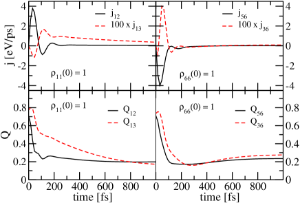
Figure 4: (Color online) Selected average energy currents $j_{ik}$ (top panels) and corresponding quantumness $Q_{ik}$ (lower panels) for FMO spectral density of Eq. (3) and $T=300$K. Notice the rescaling of the currents for better visibility.

IV.2 Classical states of energy transport

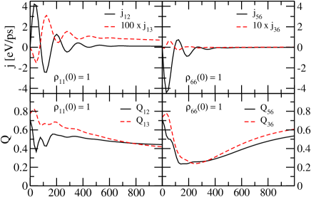
Figure 5: (Color online) Same as Fig.4, but at $T=77$K.

It has long been appreciated that the most classical states corresponding to a given quantum mechanical observable are the so-called “pointer states”. These states are “einselected” by the decoherence process due to the interaction of an environment with the system. In the case of a measurement, the environment is given by the measurement instrument, and the pointer states are in this case simply the eigenstates of the operator representing the quantum mechanical observable Zurek81 ; Zurek03 . It is in the eigenbasis of these pointer states that the density matrix becomes diagonal due to the decay of the off-diagonal matrix elements. The remaining diagonal matrix elements correspond to the probabilities of finding one of the possible outcomes of the measurement.

As eigenstates of a Hermitian operator, pointer states are pure states. The most general classical states can be obtained by classically mixing the pointer states, i.e., one chooses pointer states randomly with a certain probability. As this is a purely classical procedure, it cannot increase the “quantumness” of the system. This definition of “classicality” is well-established in quantum optics and leads to a criterion of classicality based on a well-defined positive-definite $P$-function mandel86 ; Kim05 . It was recently extended to spin-systems Giraud08 ; Giraud10 .

IV.3 Quantumness

Thus, if one wants to decide whether the energy current between two different sites in FMO has to be considered “quantum”, one has to (i) find the pointer states of the corresponding energy current operator, and (ii) check whether the state of the system $\rho(t)$ can be written as a convex combination of these pointer states. A more quantitative statement is possible by measuring the distance of $\rho(t)$ to the convex set of classical states Giraud08 ; Giraud10 ; Martin10 , i.e., here the convex hull of the pointer states. The pointer states are the eigenvectors $|v_{ik}^{l}\rangle$ of $j_{ik}$. They define the relevant pure classical states for the energy transfer along link $i-k$. Their classical mixtures form the convex set of all classical states for the energy current on link $i-k$. Any distance measure in Hilbert space is in principle suitable, and we use the Hilbert-Schmidt distance for simplicity, leading to our definition of quantumness of the current $j_{ik}$,

$$Q_{ik}(\rho)=\min_{\{p_{i}|p_{i}\geq 0,\sum_{i}p_{i}=1\}}||\rho-\sum_{l}p_{l}|v_{ik}^{l}\rangle\langle v_{ik}^{l}|||\,$$ (14)

with $||A||=({\rm tr}AA^{\dagger})^{1/2}$. Note that this measure of “quantumness” is completely analogous to and on the same level of abstraction as the measure of entanglement based on the distance of a state to the convex set of separable states (see p.363 in Ref. Bengtsson06 ), but has the advantage of being meaningful even in the single-excitation sector, and without artificially separating the system into two subsystems.
A finite value of $Q_{ik}$ means that the state cannot be written as a convex sum of pointer-states of the energy current operator $j_{ik}$, i.e., there are coherences left in $\rho(t)$ written in the pointer basis. This means essentially, that the system is in a Schrödinger-like cat state of different energy-current pointer states at a given time $t$.

By definition, $Q(\rho)\geq 0$, and $Q(\rho)=0$ if $\rho$ is classical. An upper bound is given by $Q(\rho)\leq Q_{\rm max}\equiv\sqrt{{\rm tr}\rho^{2}-1/d}$, where $d$ is the dimension of the Hilbert space Giraud10 ($Q_{\rm max}\simeq 0.925$ for pure states and $d=7$). We have calculated the quantumness $Q_{ik}(t)$ for all energy currents $\langle j_{ik}(t)\rangle$. As discussed above the currents out of the entrance site towards its strongest coupled neighbor ($j_{12}$ for $\rho_{11}(0)=1$ and $j_{56}$ for $\rho_{66}(0)=1$) have by far the largest amplitude and all currents show initial oscillations which are more pronounced at 77K than at 300K (see Fig. 4 and Fig. 5) on time scales comparable to coherent oscillations discussed above. These oscillations go hand-in-hand with substantial quantumness: $Q_{12}$ and $Q_{13}$ are initially of the order of $Q\simeq 0.6-0.8$, but drop within $\sim 100$fs to $Q\simeq 0.2-0.4$, with the exception of the case ($\rho_{11}(0)=1$, $T=77$K), where $Q_{13}$ drops slowly over 1000fs, much more slowly than the oscillations of the energy current, and the rapid decay of coherences in the site basis not withstanding. After this initial phase energy currents between all sites are small but finite (as exemplary shown by $j_{13}$ and $j_{36}$) and persist up to 1000fs and, noteworthy, a substantial amount of quantumness of the order $Q\simeq 0.2-0.4$ still persists at 1000fs as well. In the last graph ($\rho_{66}(0)=1$, $T=77$K), the quantumness even rises again after the initial drop.

This implies that the superposition of the pointer states of the energy current operator remains largely coherent even after population dynamics does not show coherence anymore. Nature has apparently engineered the environment of the FMO complex in such a way that it is rather inefficient in decohering superpositions of energy currents. Thus even though the actual currents, which bring the system into thermal equilibrium, are rather small (after the initial oscilatory phase), they turn out to have a finite quantumness. This is further illustrated by comparing with the quantumness of the thermal equilibrium state $\rho_{T}=\exp(-H_{\rm FMO}/k_{B}T)$ at $T=77$K and $T=300$K, which is of the order 0.01 and 0.002, respectively. Altogether, our data quantitatively show the non-classical nature of the energy transfer in FMO, and provide a clear physical picture of the quantumness: energy transport in FMO happens largely through a coherent Schrödinger-cat like superposition of pointer states of the energy current operator.

V Conclusion

To summarize, we have obtained numerically exact results for the real-time exciton dynamics of the FMO complex in presence of realistic environmental vibronic fluctuations. We have used the most accurate form of the spectral density realized in nature. It includes vibronic effects via a strongly localized Huang-Rhys mode. The resulting coherence times of the populations are shorter than observed experimentally. The energy transfer dynamics is also intrinsically quantum mechanical on the time scales of several hundred femtoseconds. This has been shown by calculating the quantumness as distance to the convex hull of pointer states of the energy current. The energy transport in FMO is to a large extent through a coherent Schrödinger-cat like superposition of the pointer states.

References

- (1) H. van Amerongen, L. Valkunas, and R. van Grondelle, Photosynthetic Excitons (Singapore, World Scientific, 2000).
- (2) V. May and O. Kühn, Charge and Energy Transfer Dynamics in Molecular Systems, 2nd ed. (Wiley-VCH, Weinheim, 2004).
- (3) G. S. Engel, T. R. Calhoun, E. L. Read, T. K. Ahn, T. Mančal, Y.-C. Cheng, R. E. Blankenship, and G. R. Fleming, Nature 446, 782 (2007).
- (4) G. Panitchayangkoon, D. Hayes, K. A. Fransted, J. R. Caram, E. Harel, J. Wen, R. E. Blankenship, and G.S. Engel, Proc. Natl. Acad. Sci. USA 107 12766 (2010).
- (5) R.E. Fenna and B.W. Matthews, Nature 258, 573 (1975).
- (6) M.T.W. Milder, B. Brüggemann, R. van Grondelle, and J. L. Herek, Photosynth. Res. 104, 257 (2010).
- (7) E. Collini, C.Y. Wong, K.E. Wilk, P.M.G. Curmi, P. Brumer, and G.D. Scholes, Nature 463, 644 (2010).
- (8) P. Reineker, in Exciton Dynamics in Molecular Crystals and Aggregates, Springer Tracts in Modern Physics, vol. 94 (Springer, Berlin, 1982).
- (9) L. Z. Sharp, D. Egorova, and W. Domcke, J. Chem. Phys. 132, 014501 (2010).
- (10) A. Ishizaki and G. R. Fleming, J. Chem. Phys. 130, 234110 (2009).
- (11) P. Nalbach and M. Thorwart, J. Chem. Phys. 132, 194111 (2010).
- (12) B. Palmieri, D. Abramavicius, and S. Mukamel, J. Chem. Phys. 130, 204512 (2009).
- (13) S. Jang, Y.-C. Cheng, D. R. Reichman, and J. D. Eaves, J. Chem. Phys. 129, 101104 (2008).
- (14) A. Ishizaki and G. R. Fleming, Proc. Natl. Acad. Sci. 106, 17255 (2009).
- (15) J. Prior, A.W. Chin, S.F. Huelga, and M.B. Plenio, Phys. Rev. Lett. 105, 050404 (2010).
- (16) J. Adolphs and T. Renger, Biophys. J. 91, 2778 (2006).
- (17) M. Wendling, T. Pullerits, M. A. Przyjalgowski, S.I.E. Vulto, T.J. Aartsma, R. van Grondelle, and H. van Amerongen, J. Phys. Chem. B 104, 5825 (2000).
- (18) N. Makri and D. E. Makarov, J. Chem. Phys. 102, 4600 (1995).
- (19) M. Thorwart, P. Reimann, P. Jung, and R. F. Fox, Chem. Phys. 235, 61 (1998).
- (20) M. Sarovar, A. Ishizaki, G.R. Fleming, and B. Whaley, Nature Phys. 6, 462 (2010).
- (21) C.W.J. Beenakker, in Quantum Computers, Algorithms and Chaos, Proc. Int. School of Phys. “Enrico Fermi” (Bologna, Soc. Ital. di fisica, 2006).
- (22) M. M. Wilde, J. M. McCracken, and A. Mizel, Proc. R. Soc. A 466, p.1347 (2010)
- (23) O. Giraud, P. Braun, and D. Braun, New J. Phys. 12, 063005 (2010).
- (24) W. H. Zurek, Phys. Rev. D 24, 1516 (1981).
- (25) C. Olbrich, J. Strumpfer, K. Schulten, and U. Kleinekathöfer, J. Chem. Phys. B 115, 758 (2011).
- (26) C. Olbrich and U. Kleinekathöfer, J. Phys. Chem. B 114, 12427 (2010).
- (27) Nalbach, P.; Eckel, J.; Thorwart, M. New J. Phys. 2010, 12, 065043.
- (28) J. Wen, H. Zhang, M. L. Gross, and R. E. Blankenship, Proc. Natl. Acad. Sci. 106, 6134 (2009).
- (29) E. N. Zimanyi and R. J. Silbey, J. Chem. Phys. 133, 144107 (2010).
- (30) M.O. Scully and M.S. Zubairy, Quantum Optics, (Cambridge University Press, Cambridge, 1997)
- (31) O. Giraud, P. Braun, and D. Braun, Phys. Rev. A 78, 042112 (2008).
- (32) M. S. Kim et al., Phys. Rev. A 71, 043805 (2005).
- (33) L. Mandel, Physica Scripta T 12, 34 (1986).
- (34) R. J. Hardy, Physical Review 132, 168 (1963)
- (35) J. Deppe, J. L. Feldman, Phys. Rev. B 50, 6479 (1994).
- (36) D. Segal, A. Nitzan, P. Hänggi, J. Chem. Phys. 119, 6840 (2003).
- (37) P. B. Allen, J. L. Feldman, Phys. Rev. B 48, 12581 (1993).
- (38) D. M. Leitner, J. Chem. Phys. 130, 195101 (2009).
- (39) L. Wu, D. Segal, J. Phys. A 42, 025302 (2009).
- (40) W. H. Zurek, Rev. Mod. Phys. 75, 715 (2003).
- (41) L. Mandel, Phys. Scr. T 12, 34 (1986).
- (42) M. S. Kim, E. Park, P. L. Knight, H. Jeong, Phys. Rev. A 71, 043805 (2005).
- (43) J. Martin, O. Giraud, P. A. Braun, D. Braun, and T. Bastin, Phys. Rev. A 81, 062347 (2010).
- (44) I. Bengtsson, K. Życzkowski, Geometry of quantum states: an introduction to quantum entanglement (Cambride University Press, 2006).