The Hilbert series of U/SU SQCD and Toeplitz Determinants

Abstract

We present a new technique for computing Hilbert series of ${\cal N}=1$ supersymmetric QCD in four dimensions with unitary and special unitary gauge groups. We show that the Hilbert series of this theory can be written in terms of determinants of Toeplitz matrices. Applying related theorems from random matrix theory, we compute a number of exact Hilbert series as well as asymptotic formulae for large numbers of colours and flavours – many of which have not been derived before.

1 Introduction and summary

Given a supersymmetric gauge theory, the space of solutions of the vacuum equations, known as the moduli space of vacua or simply the moduli space, is one of the first properties one can study. The phase structure and the possible excitations at a given vacuum configuration can be investigated. In supersymmetric gauge theories, holomorphic gauge invariant operators play a central role in giving us information about the structure of the moduli space. It is therefore worthwhile to study and count these holomorphic functions. This can be done in a similar fashion to statistical mechanics, i.e. by constructing a partition function. Mathematically, this partition function is known as the Hilbert series (see e.g. Forcella:2009bv ; Hanany:2007zz for reviews of applications of the Hilbert series to gauge theories and string theory). The Hilbert series not only contains information about the spectrum of the operators in the theory, it also carries geometrical properties of the moduli space (see e.g. Benvenuti:2006qr ; Feng:2007ur ; Gray:2008yu ). It is also an indicator of whether the moduli space is Calabi-Yau (see e.g.  Forcella:2008bb ; Gray:2008yu ; Hanany:2008kn ). Moreover, Hilbert series can be used as a primary tool to test various dualities in gauge theories and in string theory (see e.g.  Romelsberger:2005eg ; Forcella:2008ng ; Davey:2009sr ; Hanany:2010qu ).

The Hilbert series was first applied to study the moduli space of ${\cal N}=1$ Supersymmetric Quantum Chromodynamics (SQCD) in four dimensions by Pouliot in 1998 Pouliot:1998yv . In that paper, a method for computing the Hilbert series using the Molien–Weyl formula was briefly discussed and the Hilbert series of $SU(2)$ SQCD up to 3 flavours were explicitly stated. In 2005, Römelsberger Romelsberger:2005eg computed the Hilbert series for $SU(2)$ with 3 flavours and used it to verify the Seiberg duality. Later, in Gray:2008yu ; Hanany:2008kn , the Hilbert series were explicitly computed for SQCD with classical gauge groups for various numbers of colours and flavours and from which several geometrical aspects of the moduli space were extracted. In addition to SQCD, there have been several applications of the Hilbert series to study a wide range of supersymmetric gauge theories and string theory, e.g.  quiver gauge theories on D3-branes Forcella:2007wk ; Butti:2007jv , ${\cal N}=4$ gauge theory in four dimensions Dolan:2007rq , SQCD with one adjoint chiral superfield Hanany:2008sb , M2-brane theories Hanany:2008qc ; Hanany:2008fj ; Davey:2009sr ; Davey:2009qx ; Davey:2011mz , perturbative string spectrum Hanany:2010da , moduli spaces of instantons Nakajima:2003pg ; Benvenuti:2010pq , and a number of ${\cal N}=2$ gauge theories in four dimensions Benvenuti:2010pq ; Hanany:2006uc ; Hanany:2010qu .

In this paper, we focus on the Hilbert series of SQCD with the gauge groups $U(N_{c})$ and $SU(N_{c})$ and $N_{f}$ flavours of fundamental matters. Similarly to Gray:2008yu , the Molien–Weyl formula is used as a starting point of the computations. However, instead of evaluating the Hilbert series case by case for each $(N_{f},N_{c})$ as in Gray:2008yu , we take another approach of computations. First, we show that the Molien–Weyl formula for $U(N_{c})$ and $SU(N_{c})$ SQCD can be rewritten in terms of determinants of Toeplitz matrices. Then, we evaluate these determinants both exactly and asymptotically for a large class of values of $N_{f}$ and $N_{c}$ using several theorems from random matrix theory. In particular, such theorems are stated in §2.2.2 for $U(N_{c})$ SQCD and in §3.2 for $SU(N_{c})$ SQCD (see e.g. BottcherWidom for a mathematical review).

Since a different method from Gray:2008yu is used to compute Hilbert series in this paper, the way our results presented here is generally distinct from that in Gray:2008yu . In this paper, the Hilbert series are computed for a class of values of $N_{f}$ and $N_{c}$ rather than a specific value of $(N_{f},N_{c})$ – for example, the exact Hilbert series for $SU(N_{c})$ SQCD with $N_{f}=N_{c}$ and $N_{f}=N_{c}+1$ are presented respectively in §3.2.3 and §3.2.4 and such results, of course, apply for any $N_{c}>1$. As a consequence, many general results conjectured in Gray:2008yu can be proven (or at least can be checked in a non-trivial way) using Toeplitz determinants. Such a technique also allows us to compute explicity asymptotic formulae for large $N_{f}$ and $N_{c}$. A number of exact and asymptotic results presented in this paper are too difficult or impossible to be derived using the method in Gray:2008yu , partly due to a large number of contour integrals in the Molien–Weyl formula and partly due to the complications of the results themselves.

Let us summarise the main results and key features of this paper below.

Outline and key Points:

• In §2.2.1, we give the definitions of a Toeplitz matrix and a Toeplitz determinant. In §2.2.2, we state important facts, namely the CGBO formula and the strong Szegő limit theorem, which are applied to compute Toeplitz determinants for $U(N_{c})$ SQCD with $N_{f}$ flavours.

• In §2.2.3, we show that the Hilbert series for $U(N_{c})$ SQCD with $N_{f}$ flavours can be written in terms of a Toeplitz determinant of a symbol with a zero winding number.

• In §2.4, we use the CGBO formula to compute exact Hilbert series for $U(N_{c})$ SQCD with $N_{f}\leq N_{c}$, $N_{f}=N_{c}+1$, $N_{f}=N_{c}+2$ and $N_{f}=N_{c}+3$. We also conjectured the general expression (2.5) of the Hilbert series for any $N_{c}$ and any $N_{f}$ written in terms of a sum over representations of $SU(N_{f})\times SU(N_{f})$. The information about the moduli space and the chiral ring of $U(N_{c})$ SQCD can be extracted from these Hilbert series – this is summarised in §2.1.

• In §2.6.1, we study asymptotics for $N_{f},N_{c}>>1$ with a fixed finite difference $N_{f}-N_{c}>0$. The asymptotic formula for this limit is given by (2.115). In §2.6.2, we study asymptotics for $N_{f},N_{c}>>1$ with a fixed ratio $N_{f}/N_{c}\geq 1$. The asymptotic formula for this limit is given by (2.125).

• In §3.1, we show that the Hilbert series for $SU(N_{c})$ SQCD with $N_{f}$ flavours can be written in terms of a sum of 3 parts: (i) the Hilbert series of $U(N_{c})$ SQCD with $N_{f}$ flavours, (ii) Toeplitz determinants of symbols with positive winding numbers, and (iii) Toeplitz determinants of symbols with negative winding numbers. Observe that we can use previous results from $U(N_{c})$ SQCD in part (i) of the $SU(N_{c})$ SQCD Hilbert series computations.

• In §3.2, we state important facts, namely the Böttcher-Widom theorem and the Fisher-Hartwig theorem, which are applied to compute Toeplitz determinants for $SU(N_{c})$ SQCD with $N_{f}$ flavours.

• In §§3.2.2, 3.2.3 and 3.2.4, we use the Böttcher–Widom formula to compute exact Hilbert series for $SU(N_{c})$ SQCD with $N_{f}\leq N_{c}-1$, $N_{f}=N_{c}$, $N_{f}=N_{c}+1$. The first two subsections contain the proofs of (3.6), (5.3), (3.15) and (5.2) of Gray:2008yu . These exact results also provide a non-trivial test for the general formula (3.3).

• In §3.4, we apply the Fisher–Hartwig Theorem to examine asymptotics of the Hilbert series of $SU(N_{c})$ with $N_{f}$ flavours when $N_{f},N_{c}>>1$. In §3.4.1, we study asymptotics for $N_{f},N_{c}>>1$ with a fixed finite difference $N_{f}-N_{c}\geq 0$. The asymptotic formula for this limit is given by (3.193). In §3.4.2, we study asymptotics for $N_{f},N_{c}>>1$ with a fixed ratio $N_{f}/N_{c}\geq 1$. The asymptotic formula for this limit is given by (3.200).

Note added.

In the second version of this paper, the authors become aware of the use of Toeplitz determinants and related theorems in the literature on decaying D-branes; see e.g.  Balasubramanian:2004fz ; Jokela:2005ha ; Jokela:2008zh ; Jokela:2009fd ; Jokela:2010cc .

Notation for representations and characters.

We denote an irreducible representation of a group $SU(r+1)$ by a Dynkin label $[a_{1},a_{2},\ldots,a_{r}]$. For example, we denote by $[1,0,\ldots,0]$ the fundamental representation and by $[0,\ldots,0,1]$ the anti-fundamental representation. We also use the subscripts $k;L$ and $k;R$ to indicate respectively the $k$-th postitions from the left and the right, e.g.  $1_{k;L}$ in $[0,\ldots,0,1_{k;L},0,\ldots,0]$ denotes the 1 in the $k$-th position from the left.

For representations of the product group $G_{1}\times G_{2}$, we use the notation $[\ldots;\ldots]$ where the tuple to the left of the ; is the representation of $G_{1}$, and the tuple to the right of the ; is the representation of $G_{2}$.

Since a representation is determined by its character, we denote by $[a_{1},a_{2},\ldots,a_{r}]_{x}$ a character of the representation $[a_{1},a_{2},\ldots,a_{r}]$ written in terms of the variable $x_{1},\ldots,x_{r}$. Here the subscript $x$ denotes collectively the set of variables $x_{1},\ldots,x_{r}$. For example, the characters of the fundamental representation and the anti-fundamental representations of $SU(N_{f})$ are given by (2.10) and (2.11).

2 $U(N_{c})$ SQCD with $N_{f}$ flavours

Consider ${\cal N}=1$ supersymmetric $U(N_{c})$ gauge theory in four dimensions with $N_{f}$ quark $Q^{i}_{a}$ and $N_{f}$ anti-quarks $\widetilde{Q}^{a}_{i}$, where $a=1,\ldots,N_{c}$ and $i=1,\ldots,N_{f}$. Let us take the superpotential of this theory to be zero: $W=0$. The information about the gauge and global symmetries as well as how the matters transform under such symmetries is collected in Table 1 (see, e.g., Shifman:2007kd ).

	Gauge symmetry			Global symmetry
	$U(N_{c})=SU(N_{c})\times U(1)$	$SU(N_{f})_{1}$	$SU(N_{f})_{2}$	$U(1)_{B}$	$U(1)_{R}$	$U(1)_{Q}$	$U(1)_{\widetilde{Q}}$
$Q^{i}_{a}$	$[0,\ldots,0,1;-1]$	$[1,0,\ldots,0]$	$[0,\ldots,0]$	1	$\frac{N_{f}-N_{c}}{N_{f}}$	1	0
$\widetilde{Q}^{a}_{i}$	$[1,0,\ldots,0;+1]$	$[0,\ldots,0]$	$[0,\ldots,0,1]$	$-1$	$\frac{N_{f}-N_{c}}{N_{f}}$	0	$-1$

Table 1: The gauge and global symmetries of SQCD and the quantum numbers of the chiral supermultiplets. The quarks are $Q^{i}_{a}$ while the antiquarks are $\widetilde{Q}^{a}_{i}$. We also draw it as a quiver theory. The circular node represents the $U(N_{c})$ gauge symmetry while the two square nodes represent global $U(N_{f})_{1}$ and $U(N_{f})_{2}$ symmetries. Each square node gives rise to a baryonic $U(1)$ global symmetry, one of which is redundant. We thus have $U(1)_{Q,\tilde{Q}}$ that combine into the non-anomalous $U(1)_{B}$ (sum) and anomalous $U(1)_{A}$ (difference).

${\cal N}=1$ SQCD with $U(N_{c})$ gauge group posesses several interesting phenomena, e.g.  the Seiberg duality Shifman:2007kd , non-Abelian flux tubes (strings) and confinements Shifman:2007kd ; Gorsky:2007ip . Another motivation for studying this theory is that, as we shall see in §3.1, Hilbert series for $U(N_{c})$ SQCD with $N_{f}$ flavours are needed for our computations of Hilbert series of $SU(N_{c})$ SQCD with $N_{f}$ flavours.

2.1 The moduli space of vacua

In this paper, we focus on the classical moduli space of $U(N_{c})$ SQCD with $N_{f}$ flavours.

The case of $N_{f}<N_{c}$.

At the generic point of the moduli space, the $U(N_{c})$ gauge symmetry is partially broken to $U(N_{c}-N_{f})$. Thus, there are

$$N_{c}^{2}-(N_{c}-N_{f})^{2}=2N_{c}N_{f}-N_{f}^{2}$$

broken generators. The total number of degrees of freedom of the system is, of course, unaffected by this spontaneous symmetry breaking and the massive gauge bosons each eat one degree of freedom from the chiral matter via the Higgs effect. Therefore, of the original $2N_{c}N_{f}$ chiral multiplets (quarks and antiquarks), only

$$2N_{c}N_{f}-(2N_{c}N_{f}-N_{f}^{2})=N_{f}^{2}$$

gauge invariant degrees of freedom are left massless. Hence, the dimension of the moduli space is

$${\cal M}_{N_{f}<N_{c}}=N_{f}^{2}~{}.$$ (2.1)

We describe these $N_{f}^{2}$ massless degrees of freedom by a collection of gauge invariant objects, called mesons:

$$M^{i}_{j}=Q^{i}_{a}\widetilde{Q}^{a}_{j}~{},$$ (2.2)

where the mesons transform in the bi-fundamental representation

$$[1,0,\ldots,0;0,\ldots,0,1]$$

of $SU(N_{f})_{1}\times SU(N_{f})_{2}$. The moduli space is said to be freely generated by the mesons.

The case of $N_{f}\geq N_{c}$.

At the generic point of the moduli space, the $U(N_{c})$ gauge symmetry is completely broken. Thus, there are $N_{c}^{2}$ broken generators. Therefore, of the original $2N_{c}N_{f}$ chiral multiplets (quarks and antiquarks), only

$$2N_{c}N_{f}-N_{c}^{2}$$

gauge invariant degrees of freedom are left massless. Hence, the dimension of the moduli space is

$$\dim~{}{\cal M}_{N_{f}\geq N_{c}}=2N_{c}N_{f}-N_{c}^{2}~{}.$$ (2.3)

The moduli space is still generated by the mesons:

$$M^{i}_{j}=Q^{i}_{a}\widetilde{Q}^{a}_{j}~{}.$$ (2.4)

However, for $N_{f}\geq N_{c}+1$, there are non-trivial relations between these mesons. The basic relations (which generate the entire ideal of relations) can be written as

$$M^{[i_{1}}_{j_{1}}\ldots M^{i_{N_{c}+1}]}_{j_{N_{c}+1}}=0~{}.$$ (2.5)

They transform in the representation

$$[0,\ldots,0,1_{N_{c}+1;L},0,\ldots,0;0,\ldots,0,1_{N_{c}+1;R},0,\ldots,0]$$ (2.6)

of the $SU(N_{f})_{1}\times SU(N_{f})_{2}$ flavour symmetry. Note that the dimension of this representation ${N_{f}\choose N_{c}+1}^{2}$ is the number of relations between the mesons.

The case of $N_{f}=N_{c}+1$.

In this case, the representation (2.6) reduces to the trivial representation, i.e.  we have precisely one relation. Equation (2.5) becomes

$$\det M=0~{}.$$ (2.7)

From (2.3), the dimension of moduli space is

$$N_{f}^{2}-1~{}.$$ (2.8)

Since this is the number of generators (which is $N_{f}^{2}$) minus the number of relations (which is $1$), the moduli space for the case $N_{f}=N_{c}+1$ is a complete intersection.

2.2 The computations of Hilbert series

The Hilbert series of $U(N_{c})$ SQCD with $N_{f}$ flavours can be computed in two steps as follows.

Step 1.

First we consider the space of symmetric functions of quarks $Q$ and antiquarks $\widetilde{Q}$. The Hilbert series of this space can be constructed using the plethystic exponential, which is a generator for symmetrisation Benvenuti:2006qr ; Feng:2007ur . To remind the reader, we define the plethystic exponential of a multi-variable function $g(t_{1},...,t_{n})$ that vanishes at the origin, $g(0,...,0)=0$, to be

$$\mathop{\rm PE}[g(t_{1},\ldots,t_{n})]:=\exp\left(\sum_{r=1}^{\infty}\frac{1}{r}g(t_{1}^{r},\ldots,t_{n}^{r})\right)~{}.$$ (2.9)

Let $t$ be the $U(1)_{Q}$ global charge fugacity and $\widetilde{t}$ be the $U(1)_{\widetilde{Q}}$ global charge fugacity. Note that $0\leq t,\widetilde{t}<1$. Let $z_{1},\ldots,z_{N_{c}}$ be the fugacities of the $U(N_{c})$ gauge group. The character of the fundamental representation $[1,0,\ldots,0]_{+1}$ of $U(N_{c})$ can be written as $\sum_{a=1}^{N_{c}}z_{a}$, whereas the character of the antifundamental representation $[0,\ldots,0,1]_{-1}$ of $U(N_{c})$ can be written as $\sum_{a=1}^{N_{c}}z^{-1}_{a}$

Let $x_{1},\ldots,x_{N_{f}}$ be the $SU(N_{f})_{1}$ fugacities and let $y_{1},\ldots,y_{N_{f}}$ be the $SU(N_{f})_{2}$ fugacities. Explicitly, we take the character of the fundamental representation of $SU(N_{f})_{1}$ to be

$$[1,0,\ldots,0]_{x}=x_{1}+\sum_{k=1}^{N_{f}-2}\frac{x_{k+1}}{x_{k}}+\frac{1}{x_{N_{f}-1}}~{},$$ (2.10)

and take the character of the anti-fundamental representation of $SU(N_{f})_{2}$ to be

$$[0,0,\ldots,1]_{y}=\frac{1}{y_{1}}+\sum_{k=1}^{N_{f}-2}\frac{y_{k}}{y_{k+1}}+y_{N_{f}-1}~{}.$$ (2.11)

Then, the Hilbert series of the space of symmetric functions of quarks $Q$ and antiquarks $\widetilde{Q}$ can be written as

$$\mathop{\rm PE}\left[t[1,0,\ldots,0]_{x}\sum_{a=1}^{N_{c}}z_{a}^{-1}+\widetilde{t}[0,0,\ldots,1]_{y}\sum_{a=1}^{N_{c}}z_{a}\right]~{},$$ (2.12)

where $t[1,0,\ldots,0]_{x}\sum_{a=1}^{N_{c}}z_{a}^{-1}$ comes from the quarks $Q$ and $\widetilde{t}[0,0,\ldots,1]_{y}\sum_{a=1}^{N_{c}}z_{a}$ comes from the antiquarks $\widetilde{Q}$. Using the definition of the plethystic exponential and the identity $-\log(1-x)=\sum_{k=1}^{\infty}x^{k}/k$, we can write down the expression (2.12) explicitly as a rational function:

$$\prod_{a=1}^{N_{c}}\frac{1}{\left(1-tz_{a}^{-1}x_{1}\right)\prod_{k=1}^{N_{f}-2}\left(1-tz_{a}^{-1}\frac{x_{k+1}}{x_{k}}\right)\left(1-tz_{a}^{-1}x_{N_{f}-1}\right)}$$

$$\times\prod_{a=1}^{N_{c}}\frac{1}{\left(1-\widetilde{t}z_{a}\frac{1}{y_{1}}\right)\prod_{k=1}^{N_{f}-2}\left(1-\widetilde{t}z_{a}\frac{y_{k}}{y_{k+1}}\right)\left(1-\widetilde{t}z_{a}y_{N_{f}-1}\right)}~{}.$$ (2.13)

One may set $x_{1},\ldots,x_{N_{c}},y_{1},\ldots,y_{N_{c}}$ to unity (this process is called an unrefinement) and obtain

$$\prod_{a=1}^{N_{c}}\frac{1}{(1-\frac{t}{z_{a}})^{N_{f}}(1-\widetilde{t}z_{a})^{N_{f}}}~{}.$$ (2.14)

Step 2.

Since the moduli space is parametrised by gauge invariant quantities, we need to project representations associated with symmetric functions in $Q$ and $\widetilde{Q}$ discussed in Step 1 onto the trivial subrepresentation, which consists of the quantities invariant under the action of the gauge group. Using knowledge from representation theory (known as the Molien-Weyl formula – see e.g. DK ; Djokovich ), this can be done by integrating over the whole gauge group. In this section, we are interested in the $U(N_{c})$ gauge group, whose Haar measure is given by (see e.g. FH ; KS )

$$\int\mathrm{d}\mu_{U(N_{c})} = \frac{1}{N_{c}!(2\pi i)^{N_{c}}}\oint_{|z_{1}|=1}\frac{\mathrm{d}z_{1}}{z_{1}}\cdots\oint_{|z_{N_{c}}|=1}\frac{\mathrm{d}z_{N_{c}}}{z_{N_{c}}}|\Delta_{N_{c}}(z)|^{2}~{},$$ (2.15)

where

$$|\Delta_{N_{c}}(z)|^{2}=\prod_{1\leq a<b\leq N_{c}}|z_{a}-z_{b}|^{2}~{}.$$ (2.16)

The Hilbert series for $U(N_{c})$ SQCD with $N_{f}$ flavours is given by

$$g_{N_{f},U(N_{c})}(t,\widetilde{t},x,y)=\int\mathrm{d}\mu_{U(N_{c})}\mathop{\rm PE}\left[t[1,0,\ldots,0]_{x}\sum_{a=1}^{N_{c}}z_{a}^{-1}+\widetilde{t}[0,0,\ldots,1]_{y}\sum_{a=1}^{N_{c}}z_{a}\right]~{},$$

where here and henceforth we write $x$ and $y$ as collective notation for $x_{1},\ldots,x_{N_{c}}$ and $y_{1},\ldots,y_{N_{c}}$. Setting $x_{1},\ldots,x_{N_{c}}$ and $y_{1},\ldots,y_{N_{c}}$ to unity, we obtain the unrefined Hilbert series of $U(N_{c})$ SQCD with $N_{f}$ flavours:

$$g_{N_{f},U(N_{c})}(t,\widetilde{t})=\int\mathrm{d}\mu_{U(N_{c})}\prod_{a=1}^{N_{c}}\frac{1}{(1-\frac{t}{z_{a}})^{N_{f}}(1-\widetilde{t}z_{a})^{N_{f}}}~{}.$$ (2.18)

2.2.1 Toeplitz matrices and Toeplitz determinants

In this paper, we are concerned with computing the integrals (2.2) and (2.18) by means of Toeplitz matrices and their determinants. In this section, let us briefly summarise important facts which will be useful in subsequent computations. We follow BottcherWidom closely and neglect subtleties regarding convergences. We also refer the reader to BottSil for a comprehensive review on Toeplitz operators.

Let $\mathbb{T}$ be a complex unit circle and let $\phi:\mathbb{T}\rightarrow\mathbb{C}$ be a continuous function such that $\phi(z)\neq 0$ for all $z\in\mathbb{T}$ and $\phi$ has a zero winding number around zero, i.e.

$$0=\frac{1}{2\pi i}\oint_{|z|=1}\frac{\mathrm{d}z}{z}\frac{\phi^{\prime}(z)}{\phi(z)}~{}.$$ (2.19)

The Fourier coefficients $\phi_{k}$ (with $k\in\mathbb{Z}$) of $f$ is defined by

$$\phi_{k}:=\frac{1}{2\pi}\int_{0}^{2\pi}\mathrm{d}\theta f(e^{i\theta})e^{-ik\theta}=\frac{1}{2\pi i}\oint_{|z|=1}\frac{\mathrm{d}z}{z}~{}z^{-k}f(z)~{}.$$ (2.20)

The $n\times n$ Toeplitz matrix is defined by

$$T_{n}(\phi):=\left(\phi_{j-k}\right)_{j,k=1}^{n}~{}.$$ (2.21)

The function $\phi$ is sometimes referred to as the symbol of the Toeplitz matrix $T_{n}$. We are also interested in computing the determinant of the Toeplitz matrix,

$$D_{n}(\phi):=\det T_{n}(\phi)~{}.$$ (2.22)

This is called the Toeplitz determinant of the symbol $\phi$. We also define the infinite Toeplitz matrix $T(\phi)$ and the infinite Hankel matrix $H(\phi)$ as

$$T(\phi):=\left(\phi_{j-k}\right)_{j,k=1}^{\infty}~{},\qquad H(\phi):=\left(\phi_{j+k-1}\right)_{j,k=1}^{\infty}~{}.$$ (2.23)

Subsequently, we find that the following definition is useful

$$H(\widetilde{\phi}):=\left(\phi_{-j-k+1}\right)_{j,k=1}^{\infty}~{}.$$ (2.24)

2.2.2 The Geronimo-Case-Borodin-Okounkov (GCBO) formula and the strong Szegő limit theorem

There are theorems which are very useful for computing Toeplitz determinants (see, e.g., BasorWidom ; BottcherWidom ). Before stating these theorems, let us give more definitions which will be extensively referred to later.

Under general conditions $\phi$ can be written as

$$\phi=\phi_{+}\phi_{-}~{},$$ (2.25)

where $\phi_{+}$ (resp. $\phi_{-}$) is a nonzero analytic function in the interior (resp. exterior) of $\mathbb{T}$. This is factorisation is known as the Wiener-Hopf factorisation. Let us define the functions

$$U:=\frac{\phi_{-}}{\phi_{+}}~{},\qquad V:=\frac{\phi_{+}}{\phi_{-}}~{}.$$ (2.26)

Define the Fourier coefficients of $U$ and $V$ as

$$U_{n}:=\frac{1}{2\pi i}\oint_{|z|=1}\mathrm{d}z\left(\frac{\phi_{-}}{\phi_{+}}\right)z^{-n-1},\qquad V_{n}:=\frac{1}{2\pi i}\oint_{|z|=1}\mathrm{d}z\left(\frac{\phi_{+}}{\phi_{-}}\right)z^{-n-1}~{}.$$ (2.27)

We also define

$$G(\phi):=\exp(\log\phi)_{0}=\exp\left(\frac{1}{2\pi i}\oint_{|z|=1}\mathrm{d}z~{}z^{-1}\log\phi\right)~{}.$$ (2.28)

Define the projection matrices $P_{k}$ and $Q_{k}$ to be infinite matrices such that

$$P_{k}=\mathrm{diag}(\underbrace{1,1,\ldots,1}_{k~{}\text{ones}},0,0,\ldots)~{},\quad Q_{k}=\mathrm{diag}(\underbrace{0,0,\ldots,0}_{k~{}\text{zeros}},1,1,\ldots)~{}.$$ (2.29)

Now let us state the theorems. For the proofs, we refer the reader to BottcherWidom .

Theorem 2.1.

(The Geronimo-Case-Borodin-Okounkov (GCBO) formula. Geronimo:1979iy ; ref:BO ) The operator $\mathbf{1}-H(b)H(\widetilde{c})$ is invertible and the $n\times n$ Toeplitz determinant of the symbol $\phi$ is given by

$$D_{n}(\phi) = G(\phi)^{n}E(\phi)\det(\mathbf{1}-Q_{n}H(b)H(\widetilde{c})Q_{n})$$ (2.30)

$$= G(\phi)^{n}E(\phi)\det(\mathbf{1}-K_{n})~{},$$

where the $(i,j)$-entry of the infinite matrix $K_{n}$ is

$$K_{n}(i,j)=\left\{\begin{array}[]{ll}\sum_{k=1}^{\infty}U_{i+k}V_{-j-k}&\text{if~{} $i,j\geq n$}\\ 0&\text{otherwise}~{},\end{array}\right.$$ (2.33)

and

$$E(\phi) = \exp\left(\sum_{k=1}^{\infty}k(\log\phi)_{k}(\log\phi)_{-k}\right)~{}.$$ (2.34)

Theorem 2.2.

(The Szegő strong limit theorem. ref:szego ) In the limit of large $n$, we have

$$D_{n}(\phi)\sim G(\phi)^{n}E(\phi)~{},$$ (2.35)

where $G(\phi)$ is defined as in (2.28) and $E(\phi)$ is defined as in (2.34) .

In the following subsections, we give explicit examples on how to apply these theorems to compute Hilbert series of $U(N_{c})$ SQCD with $N_{f}$ flavours.

2.2.3 The Hilbert series and the Toeplitz determinant

Now let us go back to our problem of computing (2.2) and (2.18). Let

$$\phi(t,\widetilde{t},x,y,z)=\mathop{\rm PE}\left[t[1,0,\ldots,0]_{x}z^{-1}+\widetilde{t}[0,0,\ldots,1]_{y}z\right]~{}.$$ (2.36)

Note that $\phi(t,\widetilde{t},x,y,z)$ is non-zero for all $z\in\mathbb{T}$ and it has a zero winding number around $z=0$. The Hilbert series can be written as

$$g_{N_{f},U(N_{c})}(t,\widetilde{t},x,y) = \int\mathrm{d}\mu_{U(N_{c})}(z_{1},\ldots,z_{N_{c}})\prod_{a=1}^{N_{c}}\phi(t,\widetilde{t},x,y,z_{a})~{}.$$ (2.37)

It is well-known that the $U(N_{c})$ Haar measure can be written in terms of a determinant. For the sake of completeness and ease of reading, we include a proof in Appendix A. In particular, from (A.206), we find that

$$\int\mathrm{d}\mu_{U(N_{c})}=\det\left(\frac{1}{2\pi i}\oint_{|z|=1}\frac{\mathrm{d}z}{z}z^{a-b}\right)_{1\leq a,b\leq N_{c}}~{},$$ (2.38)

and, from (A.209), we have

$$g_{N_{f},U(N_{c})}(t,\widetilde{t},x,y) = \det\left(\frac{1}{2\pi i}\oint_{|z|=1}\frac{\mathrm{d}z}{z}z^{a-b}\phi(t,\widetilde{t},x,y,z)\right)_{1\leq a,b\leq N_{c}}$$ (2.39)

$$= D_{N_{c}}(\phi)~{}.$$

This is simply the $N_{c}\times N_{c}$ Toeplitz determinant with the symbol $\phi(t,\widetilde{t},x,y,z)$. We therefore take $n$ in Theorem 2.1 and Theorem 2.2 to be the number of colours $N_{c}$.

Results for any $N_{f}$ and any $N_{c}$.

Before we proceed, let us state some useful results for future references. The following statements are true for any $N_{f}$ and any $N_{c}$,

$$G(\phi) = \exp\left(\frac{1}{2\pi i}\oint_{|z|=1}\frac{\mathrm{d}z}{z}~{}\log\phi(t,\widetilde{t},x,y,z)\right)=1~{},$$ (2.40)

$$E(\phi) = \mathop{\rm PE}\left[[1,0,\ldots,0;0,\ldots,0,1]_{x;y}t\widetilde{t}\right]~{},$$ (2.41)

where the first equality can be easily checked and the second equality will be proven in the next subsection.

Let us now look at various cases of $N_{f}$ and $N_{c}$.

2.3 The strong Szegő limit theorem for the $N_{c}>>N_{f}$ limit

In the case, it follows from the strong Szegő limit theorem that

$$\log g_{N_{c}>>N_{f}}(t,\widetilde{t},x,y)\sim\sum^{\infty}_{k=1}k(\log\phi)_{k}(\log\phi)_{-k}~{},$$ (2.42)

where, for $n\in\mathbb{Z}$, $(\log\phi)_{n}$ is defined to be the $n$-th Fourier coefficient of $\log\phi$:

$$(\log\phi)_{n}:=\frac{1}{2\pi i}\oint_{|z|=1}\mathrm{d}zz^{-n-1}\log\phi~{}.$$ (2.43)

This can be evaluated exactly as

$$(\log\phi)_{n}=\left\{\begin{array}[]{ll}\frac{1}{n}[0,\ldots,0,1]_{y^{n}}\widetilde{t}^{n}&\text{if~{} $n>0$}\\ 0&\text{if~{} $n=0$}\\ \frac{1}{|n|}[1,0,\ldots,0]_{x^{|n|}}t^{|n|}&\text{if~{} $n<0$}~{}.\end{array}\right.$$ (2.47)

where $[0,\ldots,0,1]_{y^{n}}=\frac{1}{y_{1}^{n}}+\frac{y_{2}^{n}}{y_{1}^{n}}+\ldots\frac{y_{N_{f}-2}^{n}}{y_{N_{f}-1}^{n}}+y_{N_{f}-1}^{n}$, and similarly for $[1,0,\ldots,0]_{x^{|n|}}$. Hence, it follows from (2.34) that

$$E(\phi) = \exp\left(\sum^{\infty}_{k=1}\frac{1}{k}[1,0,\ldots,0;0,\ldots,0,1]_{x^{k};y^{k}}(t\widetilde{t})^{k}\right)$$ (2.48)

$$= \mathop{\rm PE}\left[[1,0,\ldots,0;0,\ldots,0,1]_{x;y}t\widetilde{t}\right]~{}.$$

It follows immediately from Theorem 2.2 and (2.40) that

$$g_{N_{c}>>N_{f}}(t,\widetilde{t},x,y)\sim E(\phi)=\mathop{\rm PE}\left[[1,0,\ldots,0;0,\ldots,0,1]_{x;y}t\widetilde{t}\right]~{}.$$ (2.49)

This formula can also be written in terms of sums of irreducible representations as

$$g_{N_{c}>>N_{f}}(t,\widetilde{t},x,y)\sim\frac{1}{1-(t\widetilde{t})^{N_{f}}}\times$$

$$\sum_{n_{1},\ldots,n_{N_{f}-1}=0}^{\infty}[n_{1},n_{2},\ldots,n_{N_{f}-1}~{};~{}n_{N_{f}-1},\ldots,n_{2},n_{1}](t\widetilde{t})^{\sum_{j=1}^{N_{f}-1}jn_{j}}~{}.$$ (2.50)

The unrefined Hilbert series.

Setting $x_{1},\ldots,x_{N_{c}}$ and $y_{1},\ldots y_{N_{c}}$ to unity in (2.48), we replace the representations by their dimensions. Note that

$$\dim[1,0,\ldots,0]=\dim[0,\ldots,0,1]=N_{f}~{}.$$ (2.51)

Hence, we have the unrefined Hilbert series:

$$g_{N_{c}>>N_{f}}(t,\widetilde{t},1,1)\sim\mathop{\rm PE}[N_{f}^{2}~{}t\widetilde{t}]=\frac{1}{(1-t\widetilde{t})^{N_{f}^{2}}}~{}.$$ (2.52)

In the next subsection, we use the GCBO formula to show that (2.48) and (2.52) are actually exact for $N_{f}\leq N_{c}$. In other words, corrections to the asymptotic formula (2.48) and (2.52) are indeed zero for $N_{f}\leq N_{c}$.

2.4 The GCBO formula and exact results

We perform the Wiener-Hopf factorisation of $\phi$ as

$$\phi(t,\widetilde{t},x,y,z)=\phi_{+}(t,y,z)\phi_{-}(\widetilde{t},x,z)~{},$$ (2.53)

where

$$\phi_{+}(t,y,z)=\mathop{\rm PE}\left[\widetilde{t}[0,0,\ldots,1]_{y}z\right],\qquad\phi_{-}(\widetilde{t},x,z)=\mathop{\rm PE}\left[t[1,0,\ldots,0]_{x}z^{-1}\right]~{}.$$

Using (2.27), we find that $U_{n}$ and $V_{n}$ can be evaluated exactly. For $0\leq n\leq N_{f}$,

$$U_{n} = (-\widetilde{t})^{n}\sum_{m=0}^{N_{f}-n}[m,0,\ldots,0~{};~{}0,\ldots,0,1_{(n+m);R},0,\ldots,0]_{x;y}(-t\widetilde{t})^{m}~{},\qquad$$

$$V_{-n} = (-t)^{n}\sum_{m=0}^{N_{f}-n}[0,\ldots,0,1_{(n+m);L},0,\ldots,0~{};~{}0,\ldots,0,m]_{x;y}(-t\widetilde{t})^{m}~{},$$ (2.55)

where the subscripts ${(n+m);L}$ and ${(n+m);R}$ indicate respectively the $(n+m)$-th position from the left and the right. For $n\geq N_{f}+1$, we have

$$U_{n}=V_{-n}=0~{}.$$ (2.56)

Unrefined results.

Setting $x_{1},\ldots,x_{N_{c}}$ and $y_{1},\ldots y_{N_{c}}$ to unity in (2.55), we replace the representations by their dimensions. Note that

$$\dim[m,0,\ldots,0] = \dim[0,\ldots,0,m]={N_{f}+m-1\choose m}~{},$$

$$\dim[0,\ldots,0,1_{(n+m);L},0,\ldots,0] = \dim[0,\ldots,0,1_{(n+m);R},0,\ldots,0]={N_{f}\choose n+m}~{}.\qquad$$ (2.57)

For $0\leq n\leq N_{f}$, they can be written in terms of hypergeometric functions:

$$U_{n} = (-\widetilde{t})^{n}\sum_{m=0}^{N_{f}-n}{N_{f}+m-1\choose m}{N_{f}\choose n+m}(-t\widetilde{t})^{m}\qquad$$ (2.58)

$$= (-\widetilde{t})^{n}{N_{f}\choose n}{}_{2}F_{1}(n-N_{f},N_{f};n+1;t\widetilde{t})~{},$$

$$V_{-n} = (-t)^{n}\sum_{m=0}^{N_{f}-n}{N_{f}+m-1\choose m}{N_{f}\choose n+m}(-t\widetilde{t})^{m}$$ (2.59)

$$= (-t)^{n}{N_{f}\choose n}{}_{2}F_{1}(n-N_{f},N_{f};n+1;t\widetilde{t})~{}.$$

For $n\geq N_{f}+1$, we have

$$U_{n}=V_{-n}=0~{}.$$ (2.60)

The exact Hilbert series.

The GCBO formula states that the exact formula for $g_{N_{f},U(N_{c})}$, for any $N_{c}$ and $N_{f}$, is given by

$$g_{N_{f},U(N_{c})}(t,\widetilde{t},x,y)=\det(\mathbf{1}-K_{N_{c}})\mathop{\rm PE}\left[[1,0,\ldots,0;0,\ldots,0,1]_{x;y}t\widetilde{t}\right]~{}.$$ (2.61)

Hence, the Hilbert series for any $N_{c}$ and $N_{f}$ is simply the Hilbert series for $N_{f}\leq N_{c}$ multiplied by a correction factor $\det(\mathbf{1}-K_{N_{c}})$. In the following subsections, we compute this correction exactly and asymptotically in various cases.

2.4.1 The case of $N_{f}\leq N_{c}$

Let us apply the GCBO formula to the case of $N_{f}\leq N_{c}$. From (2.33) and (2.56), we have

$$K_{N_{c}}(i,j)=0\quad\text{for all $i,j$}~{},$$ (2.62)

It is easy to see that

$$\det(\mathbf{1}-K_{N_{c}})=1~{}.$$ (2.63)

Thus, from (2.61), the refined Hilbert series is given by

$$g_{N_{f}\leq N_{c}}(t,\widetilde{t},x,y)=\mathop{\rm PE}\left[[1,0,\ldots,0;0,\ldots,0,1]_{x;y}t\widetilde{t}\right]$$

$$=\frac{1}{1-(t\widetilde{t})^{N_{f}}}\sum_{n_{1},\ldots,n_{N_{f}-1}=0}^{\infty}[n_{1},n_{2},\ldots,n_{N_{f}-1};n_{N_{f}-1},\ldots,n_{2},n_{1}](t\widetilde{t})^{\sum_{j=1}^{N_{f}-1}jn_{j}}~{}.\qquad$$ (2.64)

The unrefined Hilbert series is

$$g_{N_{f}\leq N_{c}}(t,\widetilde{t},1,1)=\frac{1}{(1-t\widetilde{t})^{N_{f}^{2}}}~{}.$$ (2.65)

Indeed, for $N_{f}\leq N_{c}$, the moduli space is of $N_{f}^{2}$ dimensional and is freely generated by the mesons.

2.4.2 The case of $N_{f}=N_{c}+1$

Let us focus on the case of $N_{f}=N_{c}+1$. Using (2.33), (2.55) and (2.56), we find that

$$K_{N_{c}}(i,j)=\left\{\begin{array}[]{ll}U_{N_{c}+1}V_{-N_{c}-1}&\text{if~{} $i=N_{c}$ and $j=N_{c}$}\\ 0&\text{otherwise}~{}.\end{array}\right.$$ (2.68)

Thus, we have

$$K_{N_{c}}(i,j)=\left\{\begin{array}[]{ll}t^{N_{f}}\widetilde{t}^{N_{f}}&\text{if~{} $i=j=N_{c}$ }\\ 0&\text{otherwise}~{},\end{array}\right.$$ (2.71)

and so

$$\det(\mathbf{1}-K_{N_{c}})=1-(t\widetilde{t})^{N_{f}}~{}.$$ (2.72)

Thus, from (2.61), the refined Hilbert series is given by

$$g_{N_{f},U(N_{f}-1)}(t,\widetilde{t},x,y)=(1-(t\widetilde{t})^{N_{f}})\mathop{\rm PE}\left[[1,0,\ldots,0;0,\ldots,0,1]_{x;y}t\widetilde{t}\right]$$

$$=\sum_{n_{1},\ldots,n_{N_{f}-1}=0}^{\infty}[n_{1},n_{2},\ldots,n_{N_{f}-1};n_{N_{f}-1},\ldots,n_{2},n_{1}](t\widetilde{t})^{\sum_{j=1}^{N_{f}-1}jn_{j}}~{}.\qquad$$ (2.73)

Setting $x$’s and $y$’s to unity, we see that the unrefined Hilbert series is

$$g_{N_{f},U(N_{f}-1)}(t,\widetilde{t},1,1)=\frac{1-(t\widetilde{t})^{N_{f}}}{(1-t\widetilde{t})^{N_{f}^{2}}}~{}.$$ (2.74)

2.4.3 The case of $N_{f}=N_{c}+2$

Let us focus on the case of $N_{f}=N_{c}+2$. Using Eq. (2.33) and (2.56), we find that

$$K_{N_{c}}(i,j)=\left\{\begin{array}[]{ll}U_{N_{c}+1}V_{-N_{c}-1}+U_{N_{c}+2}V_{-N_{c}-2}&\text{if~{} $i=j=N_{c}$ }\\ U_{N_{c}+1}V_{-N_{c}-2}&\text{if~{} $i=N_{c}$, $j=N_{c}+1$}\\ U_{N_{c}+2}V_{-N_{c}-1}&\text{if~{} $i=N_{c}+1$, $j=N_{c}$}\\ U_{N_{c}+2}V_{-N_{c}-2}&\text{if~{} $i=N_{c}+1$, $j=N_{c}+1$}\\ 0&\text{otherwise}~{}.\end{array}\right.$$ (2.80)

Using (2.55), we find that

$$K_{N_{c}}(N_{c},N_{c}) = K_{N_{c}}(N_{f}-2,N_{f}-2)$$

$$= [1,0,\ldots,0]_{x}[0,\ldots,0,1]_{y}(t\widetilde{t})^{N_{f}+1}$$

$$-\left([1,0,\ldots,0,1]_{x}+[1,0,\ldots,0,1]_{y}+1\right)(t\widetilde{t})^{N_{f}}$$

$$+[0,\ldots,0,1]_{x}[1,0,\ldots,0]_{y}(t\widetilde{t})^{N_{f}-1}~{},$$

$$K_{N_{c}}(N_{c},N_{c}+1) = K_{N_{c}}(N_{f},N_{f}-1)$$

$$= [1,0,\ldots,0]_{x}\widetilde{t}^{N_{f}}t^{N_{f}+1}-[1,0,\ldots,0]_{y}\widetilde{t}^{N_{f}-1}t^{N_{f}}$$

$$K_{N_{c}}(N_{c}+1,N_{c}) = K_{N_{c}}(N_{f}-1,N_{f})$$

$$= [0,0,\ldots,1]_{y}t^{N_{f}}\widetilde{t}^{N_{f}+1}-[0,0,\ldots,1]_{x}t^{N_{f}-1}\widetilde{t}^{N_{f}}$$

$$K_{N_{c}}(N_{c}+1,N_{c}+1) = K_{N_{c}}(N_{f}-1,N_{f}-1)$$ (2.81)

$$= (t\widetilde{t})^{N_{f}}~{},$$

and $K_{N_{c}}(i,j)=0$, otherwise. Therefore, we obtain

$$\det(\mathbf{1}-K_{N_{c}})=1-[0,\ldots,0,1;1,0,\ldots,0]_{x;y}(t\widetilde{t})^{N_{f}-1}$$

$$\qquad+\left([1,0,\ldots,0,1;0,\ldots,0]_{x;y}+[0,\ldots,0;1,0,\ldots,0,1]_{x;y}\right)(t\widetilde{t})^{N_{f}}$$

$$\qquad-[1,0,\ldots,0;0,\ldots,0,1]_{x;y}(t\widetilde{t})^{N_{f}+1}+(t\widetilde{t})^{2N_{f}}~{},$$ (2.82)

and the exact Hilbert series for $N_{f}=N_{c}+2$ is

$$g_{N_{f},U(N_{f}-2)}(t,\widetilde{t},x,y) = \mathop{\rm PE}\left[[1,0,\ldots,0;0,\ldots,0,1]_{x;y}t\widetilde{t}\right]\times$$ (2.83)

$$\Big{[}1-[0,\ldots,0,1;1,0,\ldots,0]_{x;y}(t\widetilde{t})^{N_{f}-1}$$

$$+\left([1,0,\ldots,0,1;0,\ldots,0]_{x;y}+[0,\ldots,0;1,0,\ldots,0,1]_{x;y}\right)(t\widetilde{t})^{N_{f}}$$

$$-[1,0,\ldots,0;0,\ldots,0,1]_{x;y}(t\widetilde{t})^{N_{f}+1}+(t\widetilde{t})^{2N_{f}}\Big{]}~{}.$$

This can be rewritten in terms of a sum of representations of $SU(N_{f})\times SU(N_{f})$ as

$$g_{N_{f},U(N_{f}-2)}(t,\widetilde{t},x,y)=\sum_{n_{1},n_{2},\ldots,n_{N_{f}-2}=0}^{\infty}(t\widetilde{t})^{\sum_{a=1}^{N_{f}-2}an_{a}}\times$$

$$\qquad\qquad\qquad[n_{1},n_{2},\ldots,n_{N_{f}-2},0;0,n_{N_{f}-2},\ldots,n_{2},n_{1}]_{x;y}~{}.$$ (2.84)

The unrefined Hilbert series.

Setting $x$’s and $y$’s to unity, we have

$$K_{N_{c}}(i,j)=\left\{\begin{array}[]{ll}(t\widetilde{t})^{N_{f}}+N_{f}^{2}(t\widetilde{t})^{N_{f}-1}(1-t\widetilde{t})^{2}&\text{if~{} $i=j=N_{f}-2$ }\\ -N_{f}\widetilde{t}^{-1}(t\widetilde{t})^{N_{f}}(1-t\widetilde{t})&\text{if~{} $i=N_{f}-2,j=N_{f}-1$ }\\ -N_{f}t^{-1}(t\widetilde{t})^{N_{f}}(1-t\widetilde{t})&\text{if~{} $i=N_{f}-1,j=N_{f}-2$ }\\ (t\widetilde{t})^{N_{f}}&\text{if~{} $i=j=N_{f}-1$ }\\ 0&\text{otherwise}~{}.\end{array}\right.$$ (2.90)

Hence, we arrive at

$$\det(\mathbf{1}-K_{N_{c}})=\left(1-\left(t\widetilde{t}\right)^{N_{f}}\right)^{2}-N_{f}^{2}\left(t\widetilde{t}\right)^{N_{f}-1}\left(1-t\widetilde{t}\right)^{2}~{}.$$ (2.91)

The unrefined Hilbert series for the $N_{f}=N_{c}+2$ is therefore

$$g_{N_{f},U(N_{f}-2)}(t,\widetilde{t})=\frac{\left(1-\left(t\widetilde{t}\right)^{N_{f}}\right)^{2}-N_{f}^{2}\left(t\widetilde{t}\right)^{N_{f}-1}\left(1-t\widetilde{t}\right)^{2}}{(1-t\widetilde{t})^{{N_{f}}^{2}}}~{}.$$ (2.92)

Examples.

We list a few examples of unrefined Hilbert series for small $N_{f}$.

$$g_{3,U(1)}(t,\widetilde{t}) = \frac{1+4t\tilde{t}+t^{2}\tilde{t}^{2}}{\left(1-t\tilde{t}\right)^{5}}~{},$$

$$g_{4,U(2)}(t,\widetilde{t}) = \frac{1+4t\tilde{t}+10t^{2}\tilde{t}^{2}+4t^{3}\tilde{t}^{3}+t^{4}\tilde{t}^{4}}{\left(1-t\tilde{t}\right)^{12}}~{},$$

$$g_{5,U(3)}(t,\widetilde{t}) = \frac{1+4t\tilde{t}+10t^{2}\tilde{t}^{2}+20t^{3}\tilde{t}^{3}+10t^{4}\tilde{t}^{4}+4t^{5}\tilde{t}^{5}+t^{6}\tilde{t}^{6}}{\left(1-t\tilde{t}\right)^{21}}~{},$$

$$g_{6,U(4)}(t,\widetilde{t}) = \frac{1+4t\tilde{t}+10t^{2}\tilde{t}^{2}+20t^{3}\tilde{t}^{3}+35t^{4}\tilde{t}^{4}+20t^{5}\tilde{t}^{5}+10t^{6}\tilde{t}^{6}+4t^{7}\tilde{t}^{7}+t^{8}\tilde{t}^{8}}{\left(1-t\tilde{t}\right)^{32}}~{}.$$

The limit $N_{f},N_{c}>>1$ and $N_{f}=N_{c}+2$.

In this limit, (2.83) becomes

$$g_{N_{f}=N_{c}+2}(t,\widetilde{t},x,y)\sim\Big{[}1-[0,\ldots,0,1;1,0,\ldots,0]_{x;y}(t\widetilde{t})^{N_{f}-1}$$

$$\qquad+\left([1,0,\ldots,0,1;0,\ldots,0]_{x;y}+[0,\ldots,0;1,0,\ldots,0,1]_{x;y}\right)(t\widetilde{t})^{N_{f}}$$

$$\qquad-[1,0,\ldots,0;0,\ldots,0,1]_{x;y}(t\widetilde{t})^{N_{f}+1}\Big{]}\mathop{\rm PE}\left[[1,0,\ldots,0;0,\ldots,0,1]_{x;y}t\widetilde{t}\right]~{}.$$ (2.94)

Unrefining this Hilbert series, we obtain

$$g_{N_{f},U(N_{f}-2)}(t,\widetilde{t})\sim\frac{1-N_{f}^{2}(1-t\widetilde{t})^{2}(t\widetilde{t})^{N_{f}-1}}{(1-t\widetilde{t})^{N_{f}^{2}}}~{}.$$ (2.95)

2.4.4 The unrefined Hilbert series for $N_{f}=N_{c}+3$

Let us focus on the case of $N_{f}=N_{c}+3$. From (2.56), (2.58) and (2.59), we find that

$$K_{N_{c}}(N_{c},N_{c}) = (t\widetilde{t})^{N_{f}}+(t\widetilde{t})^{N_{f}-2}\left(1-t\widetilde{t}\right)^{2}\left[{N_{f}\choose 2}-{N_{f}+1\choose 2}t\widetilde{t}\right]^{2}$$

$$+(t\widetilde{t})^{N_{f}-1}\left(1-t\widetilde{t}\right)^{2}N_{f}^{2}~{},$$

$$K_{N_{c}}(N_{c},N_{c}+1) = -\widetilde{t}^{-1}(t\widetilde{t})^{N_{f}}\left(1-t\widetilde{t}\right)N_{f}$$

$$-\widetilde{t}^{-1}(t\widetilde{t})^{N_{f}-1}\left(1-t\widetilde{t}\right)^{2}\left[{N_{f}\choose 2}-{N_{f}+1\choose 2}t\widetilde{t}\right]N_{f}~{},$$

$$K_{N_{c}}(N_{c},N_{c}+2) = \widetilde{t}^{-2}(t\widetilde{t})^{N_{f}}\left(1-t\widetilde{t}\right)\left[{N_{f}\choose 2}-{N_{f}+1\choose 2}t\widetilde{t}\right]~{},$$

$$K_{N_{c}}(N_{c}+1,N_{c}+1) = \left(t\widetilde{t}\right)^{-1+N_{f}}\left[t\widetilde{t}+\left(1-t\widetilde{t}\right)^{2}N_{f}^{2}\right]~{},$$

$$K_{N_{c}}(N_{c}+1,N_{c}+2) = -\widetilde{t}^{-1}(t\widetilde{t})^{N_{f}}\left(1-t\widetilde{t}\right)N_{f}~{},$$

$$K_{N_{c}}(N_{c}+2,N_{c}+2) = \left(t\widetilde{t}\right)^{N_{f}}~{},$$

and for $N_{c}+2\geq i>j\geq N_{c}$, the entry $K_{N_{c}}(i,j)$ is simply $K_{N_{c}}(j,i)$ with $t$ and $\widetilde{t}$ interchanged. Other entries of $K_{N_{c}}$ vanish.

Thus, it follows that

$$\det(\mathbf{1}-K_{N_{c}})=1-\left(t\widetilde{t}\right)^{N_{f}-2}\left[\left(1-t\widetilde{t}\right)^{2}\left[{N_{f}\choose 2}-{N_{f}+1\choose 2}t\widetilde{t}\right]^{2}+t\widetilde{t}\left(2N_{f}^{2}\left(1-t\widetilde{t}\right)^{2}+3t\widetilde{t}\right)\right]$$

$$\qquad+\left(t\widetilde{t}\right)^{2N_{f}-2}\Bigg{[}(1-{t\widetilde{t}})^{2}\left({N_{f}\choose 2}-{t\widetilde{t}}{N_{f}+1\choose 2}\right)\left({N_{f}\choose 2}-{t\widetilde{t}}{N_{f}+1\choose 2}-2(1-{t\widetilde{t}})N_{f}^{2}\right)$$

$$\qquad+N_{f}^{4}(1-t\widetilde{t})^{4}+2N_{f}^{2}(1-t\widetilde{t})^{2}t\widetilde{t}+3(t\widetilde{t})^{2}\Bigg{]}-\left(t\widetilde{t}\right)^{3N_{f}}~{}.$$ (2.96)

Thus, the Hilbert series for the $N_{f}=N_{c}+3$ case is

$$g_{N_{f},U(N_{f}-3)}(t,\widetilde{t})=\frac{\det(\mathbf{1}-K_{N_{f}-3})}{(1-t\widetilde{t})^{{N_{f}}^{2}}}~{},$$ (2.97)

where $\det(\mathbf{1}-K_{N_{f}-3})$ is given by (2.96).

Examples.

We list a few examples of unrefined Hilbert series for small $N_{f}$.

$$g_{4,U(1)} = \frac{1+9t\tilde{t}+9t^{2}\tilde{t}^{2}+t^{3}\tilde{t}^{3}}{\left(1-t\tilde{t}\right)^{7}}~{},$$

$$g_{5,U(2)} = \frac{1+9t\tilde{t}+45t^{2}\tilde{t}^{2}+65t^{3}\tilde{t}^{3}+45t^{4}\tilde{t}^{4}+9t^{5}\tilde{t}^{5}+t^{6}\tilde{t}^{6}}{\left(1-t\tilde{t}\right)^{16}}~{},$$

$$g_{6,U(3)} = \frac{1+9t\tilde{t}+45t^{2}\tilde{t}^{2}+165t^{3}\tilde{t}^{3}+270t^{4}\tilde{t}^{4}+270t^{5}\tilde{t}^{5}+165t^{6}\tilde{t}^{6}+45t^{7}\tilde{t}^{7}+9t^{8}\tilde{t}^{8}+t^{9}\tilde{t}^{9}}{\left(1-t\tilde{t}\right)^{27}}~{}.$$

The limit $N_{f},N_{c}>>1$ and $N_{f}=N_{c}+3$.

To obtain the asymptotic formula, we approximate $\det(\mathbf{1}-K_{N_{c}})$ by neglecting terms of order $t^{2N_{f}}$ and smaller in comparison with those of order $t^{N_{f}}$. Expanding the square bracket in the first line of (2.96) and neglecting terms of order ${N_{f}\choose 2}$ and smaller in comparison with those of order ${N_{f}\choose 2}^{2}$, we obtain

$$g_{N_{f},U(N_{f}-3)}(t,\widetilde{t})\sim\frac{1-{N_{f}\choose 2}^{2}(1-t\widetilde{t})^{4}(t\widetilde{t})^{N_{f}-2}}{(1-t\widetilde{t})^{N_{f}^{2}}}~{}.$$ (2.99)

2.5 An exact refined Hilbert series for any $N_{f}$ and $N_{c}$

From (2.4.2) and (2.4.3), we see that one can express the Hilbert series in terms of a sum of representations of $SU(N_{f})\times SU(N_{f})$. We conjecture that the Hilbert series of $U(N_{c})$ SQCD with $N_{f}$ flavours can be written as

$$g_{N_{f},U(N_{c})}(t,\widetilde{t},x,y)=\sum_{n_{1},n_{2},\ldots,n_{N_{c}}=0}^{\infty}(t\widetilde{t})^{\sum_{a=1}^{N_{c}}an_{a}}\times$$

$$\qquad\qquad\qquad[n_{1},n_{2},\ldots,n_{N_{c}},0,\ldots,0~{};~{}0,\ldots,0,n_{N_{c}},\ldots,n_{2},n_{1}]_{x;y}~{}.$$ (2.100)

A consistency check.

We perform a non-trivial check for this formula by setting $x=y=1$ and obtain an unrefined Hilbert series which can be compared with known results. Recall the Weyl dimension formula for the $SU(n)$ irreducible representation:

$$\dim[a_{1},\ldots,a_{n-1}]=\prod_{1\leq i<j\leq n}\frac{(a_{i}+\ldots a_{j-1})+(j-i)}{j-i}~{}.$$ (2.101)

For example, let us take $N_{f}=5$ and $N_{c}=3$. Then,

$$\begin{array}[]{rcl}\dim~{}[n_{1},n_{2},n_{3},0;0,n_{3},n_{2},n_{1}]&=&\Big{[}(4!~{}3!~{}2!~{}1!)^{-1}\times\\ &&(n_{1}+1)(n_{1}+n_{2}+2)(n_{1}+n_{2}+n_{3}+3)(n_{1}+n_{2}+n_{3}+4)\times\\ &&(n_{2}+1)(n_{2}+n_{3}+2)(n_{2}+n_{3}+0+3)\times\\ &&(n_{3}+1)(n_{3}+0+2)\times\\ &&(0+1)\Big{]}^{2}~{}.\end{array}$$

From (2.5), we find that the unrefined Hilbert series for $N_{f}=5$ and $N_{c}=3$ is

$$g_{5,U(3)}(t,\widetilde{t}) = \frac{1+4t\tilde{t}+10t^{2}\tilde{t}^{2}+20t^{3}\tilde{t}^{3}+10t^{4}\tilde{t}^{4}+4t^{5}\tilde{t}^{5}+t^{6}\tilde{t}^{6}}{\left(1-t\tilde{t}\right)^{21}}~{}.$$ (2.102)

Observe that this coincides with (2.4.3).

The generators and relations.

The information about the generators of the moduli space and their relations can be extracted from the Hilbert series using the plethystic logarithm Benvenuti:2006qr ; Feng:2007ur . To remind the reader, we define the plethystic logarithm of a multi-variable function $g(t_{1},...,t_{n})$ to be

$$\mathop{\rm PL}[g(t_{1},\ldots,t_{n})]:=\sum_{k=1}^{\infty}\frac{\mu(k)}{k}\log g(t^{k}_{1},\ldots,t^{k}_{n})~{}.$$ (2.103)

where $\mu(k)$ is the Möbius function. The significance of the series expansion of the plethystic logarithm is stated in Benvenuti:2006qr ; Feng:2007ur : the first terms with plus sign give the generators while the first terms with the minus sign give the relations between these generators. Now let us compute the plethystic logarithms of various Hilbert series we have computed and interpret the results.

For $N_{f}\leq N_{c}$, we use the Hilbert series is given in the first line of (2.4.1) and so we have

$$\mathop{\rm PL}[g_{N_{f}\leq N_{c}}(t,\widetilde{t},x,y)]=[1,0,\ldots,0;0,\ldots,0,1]_{x;y}t\widetilde{t}~{}.$$ (2.104)

This indicates that the moduli space is freely generated by the mesons in the representation $[1,0,\ldots,0;0,\ldots,0,1]$ of $SU(N_{f})\times SU(N_{f})$. This agrees with the discussion in §2.1.

For $N_{f}=N_{c}+1$, we use the Hilbert series is given in the first line of (2.4.2), and so we have

$$\mathop{\rm PL}[g_{N_{c}+1,U(N_{c})}(t,\widetilde{t},x,y)]=[1,0,\ldots,0;0,\ldots,0,1]_{x;y}t\widetilde{t}-(t\widetilde{t})^{N_{c}+1}~{}.$$ (2.105)

This indicates that the moduli space is a complete intersection. The generators are the mesons in the representation $[1,0,\ldots,0;0,\ldots,0,1]$ of $SU(N_{f})\times SU(N_{f})$, and there is one relation in the trivial representation of $SU(N_{f})\times SU(N_{f})$. This also agrees with the discussion in §2.1.

For $N_{f}\geq N_{c}+2$, we use the Hilbert series is given in (2.5), and so we have

$$\mathop{\rm PL}[g_{N_{f}\geq N_{c}+2}(t,\widetilde{t},x,y)]=[1,0,\ldots,0;0,\ldots,0,1]_{x;y}t\widetilde{t}$$

$$\qquad-[0,\ldots,0,1_{N_{c}+1;L},0,\ldots,0;0,\ldots,0,1_{N_{c}+1;R},0,\ldots,0](t\widetilde{t})^{N_{c}+1}+\ldots~{}.$$ (2.106)

This indicates that the moduli space is not a complete intersection. The generators are the mesons in the representation $[1,0,\ldots,0;0,\ldots,0,1]$ of $SU(N_{f})\times SU(N_{f})$, and there are relations in the representation $[0,\ldots,0,1_{N_{c}+1;L},0,\ldots,0;0,\ldots,0,1_{N_{c}+1;R},0,\ldots,0]$ of $SU(N_{f})\times SU(N_{f})$. This also agrees with the discussion in §2.1.

2.6 Various asymptotics

In this subsection, we examine asymptotics of Hilbert series for $N_{f}>N_{c}$ when $N_{f}$ and $N_{c}$ is large. (Note that for $N_{f}\leq N_{c}$, one can simply use the exact formula (2.65).)

2.6.1 Asymptotics for $N_{f},N_{c}>>1$ with a fixed difference $N_{f}-N_{c}>0$

Let us focus on the limit of large $N_{f}$ and $N_{c}$ where the difference $N_{f}-N_{c}$ is kept fixed and being positive. For convenience, we define

$$\Delta:=N_{f}-(N_{c}+1)~{}.$$ (2.107)

We also assume that $\Delta\geq 0$ and that $\Delta$ is of order $1$.

In this limit, elements of $K_{N_{c}}$ are much smaller than $1$. Therefore,

$$\det(\mathbf{1}-K_{N_{c}})=\exp\left(\mathop{\rm Tr}\log(1-K_{N_{c}})\right)\sim\exp\left(-\mathop{\rm Tr}K_{N_{c}}\right)\sim 1-\mathop{\rm Tr}K_{N_{c}}~{}.\qquad$$ (2.108)

Now let us consider $\mathop{\rm Tr}K_{N_{c}}$. We claim that the leading contribution to $\mathop{\rm Tr}K_{N_{c}}$ comes from $U_{N_{c}+1}V_{-(N_{c}+1)}$ in the matrix element $K_{N_{c}}(N_{c},N_{c})$. Below, we show that for $0\leq m\leq\Delta-1$,

$$U_{N_{c}+1+m+1}V_{-(N_{c}+1+m+1)}\sim N_{c}^{-2}U_{N_{c}+1+m}V_{-(N_{c}+1+m)}~{}.$$ (2.109)

Note that from (2.56), for $m\geq\Delta+1$, we have $U_{N_{c}+1+m}V_{-(N_{c}+1+m)}=0$.

Proof.

Suppose that $0\leq m\leq\Delta-1$. Using (2.58) and (2.59). we obtain

$$U_{N_{c}+1+m+1}V_{-(N_{c}+1+m+1)} = {N_{f}\choose\Delta-m-1}^{2}\left[{}_{2}F_{1}(m+1-\Delta,N_{f};N_{c}+2+m+1;t\widetilde{t})\right]^{2}\times$$

$$(t\widetilde{t})^{N_{c}+1+m+1}~{}.$$

Now consider the binomial coefficient

$${N_{f}\choose\Delta-m-1} = \frac{N_{f}!}{(\Delta-m-1)!(N_{f}-\Delta+m+1)!}$$

$$= \frac{\Delta-m}{N_{f}-\Delta+m+1}{N_{f}\choose\Delta-m}$$

$$= \frac{\Delta-m}{N_{c}+2+m}{N_{f}\choose\Delta-m}~{}.$$

Hence, we find that

$$\frac{U_{N_{c}+1+m+1}V_{-(N_{c}+1+m+1)}}{U_{N_{c}+1+m}V_{-(N_{c}+1+m)}}=(t\widetilde{t})\left[\frac{\Delta-m}{N_{c}+2+m}\right]^{2}\left[\frac{{}_{2}F_{1}(m+1-\Delta,N_{f};N_{c}+2+m+1;t\widetilde{t})}{{}_{2}F_{1}(m-\Delta,N_{f};N_{c}+2+m;t\widetilde{t}))}\right]^{2}~{}.$$

The ratio between the two hypergeometric functions is of order $1$, i.e.  as $N_{c},N_{f}\rightarrow\infty$,

$$\frac{{}_{2}F_{1}(m+1-\Delta,N_{f};N_{c}+2+m+1;t\widetilde{t})}{{}_{2}F_{1}(m-\Delta,N_{f};N_{c}+2+m;t\widetilde{t}))}=O(1)~{},$$ (2.110)

and so

$$\frac{U_{N_{c}+1+m+1}V_{-(N_{c}+1+m+1)}}{U_{N_{c}+1+m}V_{-(N_{c}+1+m)}}\sim(t\widetilde{t})\left[\frac{\Delta-m}{N_{c}+2+m}\right]^{2}~{}.$$ (2.111)

Since $\Delta$ is of order 1, for a large $N_{c}$ we have

$$\frac{U_{N_{c}+1+m+1}V_{-(N_{c}+1+m+1)}}{U_{N_{c}+1+m}V_{-(N_{c}+1+m)}}\sim\frac{1}{N_{c}^{2}}~{},$$ (2.112)

as claimed. Thus, in $\mathop{\rm Tr}K_{N_{c}}$, we may neglect other diagonal elements of $K_{N_{c}}$ in comparison with $K_{N_{c}}(N_{c},N_{c})$, and the leading contribution in $K_{N_{c}}(N_{c},N_{c})$ is $U_{N_{c}+1}V_{-(N_{c}+1)}$. ∎

It follows from the above discussion that

$$\mathop{\rm Tr}K_{N_{c}} \sim K_{N_{c}}(N_{c}+1,N_{c}+1)$$ (2.113)

$$\sim U_{N_{c}+1}V_{-(N_{c}+1)}$$

$$= {N_{f}\choose\Delta}^{2}\left[{}_{2}F_{1}(-\Delta,N_{f};N_{c}+2;t\widetilde{t})\right]^{2}(t\widetilde{t})^{N_{c}+1}$$

$$\sim {N_{f}\choose\Delta}^{2}(1-t\widetilde{t})^{2\Delta}(t\widetilde{t})^{N_{c}+1}~{},$$

where we have have used the following approximation to establish the fourth equality:

$${}_{2}F_{1}(-\Delta,N_{f};N_{f}-\Delta+1;t\widetilde{t})\sim{}_{2}F_{1}(-\Delta,N_{f};N_{f};t\widetilde{t})=(1-t\widetilde{t})^{\Delta}~{}.$$ (2.114)

Thus, it follows from the CGBO formula that

$$g_{N_{f},U(N_{c})}(t,\widetilde{t}) \sim \frac{1-{N_{f}\choose\Delta}^{2}(1-t\widetilde{t})^{2\Delta}(t\widetilde{t})^{N_{c}+1}}{(1-t\widetilde{t})^{N_{f}^{2}}}~{},\qquad$$ (2.115)

for $N_{f},N_{c}>>1$ and the difference $\Delta=N_{f}-N_{c}-1\geq 0$ kept fixed.

Note that for $\Delta=0$, we recover the exact formula (2.74) for $N_{f}=N_{c}+1$. Moreover, for $\Delta=1$ and $\Delta=2$, we recover the asymptotic formulae (2.95) and (2.99), both of which are derived from the exact Hilbert series.

2.6.2 Asymptotics for $N_{f},N_{c}>>1$ with a fixed ratio $N_{f}/N_{c}\geq 1$

In this subsection, we focus on the limit $N_{f},N_{c}>>1$ with a finite ratio

$$r:=\frac{N_{f}}{N_{c}}\geq 1~{}.$$ (2.116)

Derivation of the asymptotic formula.

Let us consider (2.111). Since $\Delta=(r-1)N_{c}-1$, we see that for $0\leq m\leq\Delta-1$, we have

$$\frac{1}{rN_{c}}\leq\frac{\Delta-m}{N_{c}+2+m}\leq r-1~{}.$$ (2.117)

Hence, we see that

$$\frac{t\widetilde{t}}{r^{2}N_{c}^{2}}\lesssim\frac{U_{N_{c}+1+m+1}V_{-(N_{c}+1+m+1)}}{U_{N_{c}+1+m}V_{-(N_{c}+1+m)}}\lesssim t\widetilde{t}(r-1)^{2}$$ (2.118)

We would like the upper bound to be sufficiently small, so that we have control over $U_{N_{c}+1+m}V_{-(N_{c}+1+m)}$ for $m\geq 0$. We are interested in the following limiting cases:

• Case 1: Consider $r-1=o(1)$ as $N_{c}\rightarrow\infty$. In other words, we take $r$ to be close to $1$ and $t\widetilde{t}$ can take any value between $0$ and $1$.

• Case 2: Consider $t\widetilde{t}=o(1)$ as $N_{c}\rightarrow\infty$. In other words, we take $t\widetilde{t}$ to be small and $r$ can take any finite positive value greater than $1$.

In both cases, we see that $U_{N_{c}+1+m+1}V_{-(N_{c}+1+m+1)}$ can be neglected in comparison with $U_{N_{c}+1+m}V_{-(N_{c}+1+m)}$. Thus, the approximation

$$\det(\mathbf{1}-K_{N_{c}})\sim 1-\mathop{\rm Tr}K_{N_{c}}\sim 1-U_{N_{c}+1}V_{-(N_{c}+1)}$$ (2.119)

is valid in both limiting cases. We therefore consider

$$U_{N_{c}+1}V_{-(N_{c}+1)} = {N_{f}\choose N_{c}+1}^{2}\left[{}_{2}F_{1}(N_{c}+1-N_{f},N_{f};N_{c}+2;t\widetilde{t})\right]^{2}(t\widetilde{t})^{N_{c}+1}$$ (2.120)

$$= {rN_{c}\choose N_{c}+1}^{2}\left[{}_{2}F_{1}(-(r-1)N_{c}+1,rN_{c};N_{c}+2;t\widetilde{t})\right]^{2}(t\widetilde{t})^{N_{c}+1}~{}.\qquad$$

Unfortunately, we are not aware of a good asymptotic formula for

$${}_{2}F_{1}(-(r-1)N_{c}+1,rN_{c};N_{c}+2;t\widetilde{t})$$

in the limit of large $N_{c}$, finite $r>1$ and $0<t\tilde{t}<1$. Therefore, we leave the expression for the hypergeometric function as it is.

Therefore, we have

$$\det(\mathbf{1}-K_{N_{c}})\sim 1-{rN_{c}\choose N_{c}+1}^{2}\left[{\cal F}(N_{c},r,t\widetilde{t})\right]^{2}(t\widetilde{t})^{N_{c}+1}~{},$$ (2.123)

where ${\cal F}(N_{c},r,t\widetilde{t})$ is a shorthand notation for the hypergeometric function:

$${\cal F}(N_{c},r,t\widetilde{t}):={}_{2}F_{1}(-(r-1)N_{c}+1,rN_{c};N_{c}+2;t\widetilde{t})~{}.$$ (2.124)

The asymptotic formula.

Thus, using the GCBO formula, we obtain the required asymptotic formula

$$g_{rN_{c},U(N_{c})}(t,\widetilde{t})\sim\frac{1-{rN_{c}\choose N_{c}+1}^{2}\left[{\cal F}(N_{c},r,t\widetilde{t})\right]^{2}(t\widetilde{t})^{N_{c}+1}}{(1-t\widetilde{t})^{r^{2}N_{c}^{2}}}~{}.$$ (2.125)

We emphasise that this asymptotic formula is valid for both limiting cases described above. We provide non-trivial consistency checks for this formula in the next subsection.

Special case $r=1$:

Observe from (2.125) that as $r\rightarrow 1$, we have

$$g_{N_{c},U(N_{c})}(t,\widetilde{t})\sim\frac{1}{(1-t\widetilde{t})^{N_{c}^{2}}}~{}.$$ (2.126)

This indeed coincides with the exact result (2.65) for $N_{f}=N_{c}$.

2.6.3 Consistency checks

In this subsection, we provide consistency checks for the exact and the asymptotic formulae we have derived so far.

In Figure 1, we plot the graphs of $\log g_{N_{c}+2,U(N_{c})}(t,\widetilde{t})$ given by (2.95), (2.115) and (2.125) against $N_{c}$, with $\Delta=1$, $r=1+2/N_{c}$ and $t\widetilde{t}=0.5$. Note that, for (2.125), this is the first limiting case described in §2.6.2, since $r-1\rightarrow 0$ as $N_{c}\rightarrow\infty$. It can be see that the asymptotic formulae (2.115) and (2.125) approach the exact result (2.95) when $N_{c}$ is large.

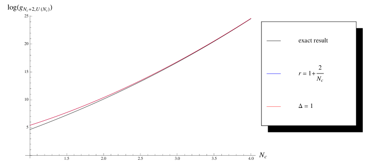
Figure 1: The case of $N_{f}=N_{c}+2$: The graphs of the exact Hilbert series (2.95) with its asymptotic formulae (2.115) and (2.125). We take $\Delta=1$, $r=1+2/N_{c}$, $t\widetilde{t}=0.5$. Note that the graphs for both asymptotic formulae are on top of each other in this figure.

In Figure 2, we plot the graphs of $\log g_{N_{c}+3,U(N_{c})}(t,\widetilde{t})$ given by (2.97), (2.115) and (2.125) against $N_{c}$, with $\Delta=2$, $r=1+3/N_{c}$ and $t\widetilde{t}=0.5$. Note that, for (2.125), this is the first limiting case described in §2.6.2, since $r-1\rightarrow 0$ as $N_{c}\rightarrow\infty$. It can be see that the asymptotic formulae (2.115) and (2.125) approach the exact result (2.97) when $N_{c}$ is large.

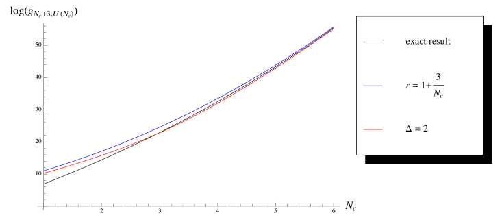
Figure 2: The case of $N_{f}=N_{c}+3$: The graphs of the exact Hilbert series (2.97) with its asymptotic formulae (2.115) and (2.125). We take $\Delta=2$, $r=1+3/N_{c}$, $t\widetilde{t}=0.5$.

In Figure 3, we plot the graphs of $\log g_{6,U(3)}(t,\widetilde{t})$ given by (2.97) and (2.125) (with $r=2$) against $t\widetilde{t}$. As we expected from the second limiting case in §2.6.2, the asymptotic formula should give a good approximation when $t\widetilde{t}=O(N_{c}^{-1})$. Indeed, as one can see from the graph, the asymptotic result is in agreement with the exact result for $t\widetilde{t}<1/N_{c}=1/3$.

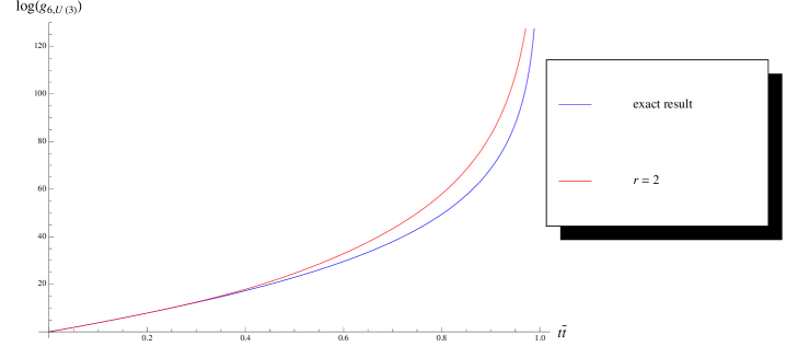
Figure 3: The case of $N_{c}=3,N_{f}=6$: The graphs of the exact Hilbert series from (2.97) and its asymptotic formula (2.125) (with $r=2$). As we expected from the second limiting case in §2.6.2, the asymptotic formula is in agreement with the exact result for $t\widetilde{t}<1/N_{c}=1/3$.

3 $SU(N_{c})$ SQCD with $N_{f}$ flavours

Consider ${\cal N}=1$ supersymmetric $SU(N_{c})$ gauge theory in four dimensions with $N_{f}$ quark $Q^{i}_{a}$ and $N_{f}$ anti-quarks $\widetilde{Q}^{a}_{i}$, where $a=1,\ldots,N_{c}$ and $i=1,\ldots,N_{f}$. The superpotential of this theory is zero: $W=0$. The information about the gauge and global symmetries as well as how the matters transform under such symmetries is collected in Table 2 .

	Gauge symmetry			Global symmetry
	$SU(N_{c})$	$SU(N_{f})_{1}$	$SU(N_{f})_{2}$	$U(1)_{B}$	$U(1)_{R}$	$U(1)_{Q}$	$U(1)_{\widetilde{Q}}$
$Q^{i}_{a}$	$[0,\ldots,0,1]$	$[1,0,\ldots,0]$	$[0,\ldots,0]$	1	$\frac{N_{f}-N_{c}}{N_{f}}$	1	0
$\widetilde{Q}^{a}_{i}$	$[1,0,\ldots,0]$	$[0,\ldots,0]$	$[0,\ldots,0,1]$	$-1$	$\frac{N_{f}-N_{c}}{N_{f}}$	0	$-1$

Table 2: The gauge and global symmetries of SQCD and the quantum numbers of the chiral supermultiplets. The quarks are $Q^{i}_{a}$ while the antiquarks are $\widetilde{Q}^{a}_{i}$. We also draw it as a quiver theory. The circular node represents the $U(N_{c})$ gauge symmetry while the two square nodes represent global $U(N_{f})_{1}$ and $U(N_{f})_{2}$ symmetries. Each square node gives rise to a baryonic $U(1)$ global symmetry, one of which is redundant. We thus have $U(1)_{Q,\tilde{Q}}$ that combine into the non-anomalous $U(1)_{B}$ (sum) and anomalous $U(1)_{A}$ (difference).

SQCD with the $SU(N_{c})$ gauge group and $N_{f}$ flavours is studied and discussed in Seiberg:1994bz ; Intriligator:1994sm ; Seiberg:1994pq ; argyres ; terning ; insei:07 ; insei:95 ; Gray:2008yu . Various geometrical aspects of the moduli space are examined in Gray:2008yu , where the Hilbert series are also computed and studied in details. In the following subsection, we present a method for computing the Hilbert series and discuss how to rewrite them in terms of Toeplitz determinants. We compare the method used in this paper with the one used in Gray:2008yu in §3.1.1.

3.1 The computations of Hilbert series

The Hilbert series for $SU(N_{c})$ SQCD with $N_{f}$ flavours can be computed in a similar way to that for $U(N_{c})$ SQCD with $N_{f}$ flavours. The first step is to construct the Hilbert series of the space of symmetric functions of quarks $Q$ and antiquarks $\widetilde{Q}$. This is given by

$$\mathop{\rm PE}\left[t[1,0,\ldots,0]_{x}\sum_{a=1}^{N_{c}}z_{a}^{-1}+\widetilde{t}[0,0,\ldots,1]_{y}\sum_{a=1}^{N_{c}}z_{a}\right]~{},$$ (3.127)

where for the $SU(N_{c})$ gauge group, one needs to impose the condition that

$$z_{1}z_{2}\ldots z_{N_{c}}=1~{}.$$ (3.128)

The second step is to integrate over the gauge group $SU(N_{c})$ in order to obtain the Hilbert series which counts gauge invariant operators. For this step, we need an appropriate Haar measure of $SU(N_{c})$ for this problem. Let us now discuss such a Haar measure.

The Haar measure.

The Haar measure of $SU(N_{c})$ can be obtained from the Haar measure of $U(N_{c})$ by restricting $z_{1}\cdots z_{N_{c}}=1$. This can be written as

$$\int\mathrm{d}\mu_{SU(N_{c})} = \frac{1}{N_{c}!(2\pi i)^{N_{c}-1}}\oint_{|z_{1}|=1}\frac{\mathrm{d}z_{1}}{z_{1}}\cdots\oint_{|z_{N_{c}}|=1}\frac{\mathrm{d}z_{N_{c}}}{z_{N_{c}}}|\Delta_{N_{c}}(z)|^{2}\delta(z_{1}\cdots z_{N_{c}}-1)~{}.\qquad$$ (3.129)

In Appendix B, we show that the delta function in this multi-contour integral can be replaced by an infinite sum as follows:

$$\delta(z_{1}\cdots z_{N_{c}}-1)\quad\longrightarrow\quad\frac{1}{2\pi i}\sum_{k=-\infty}^{\infty}z_{1}^{k}z_{2}^{k}\ldots z_{N_{c}}^{k}~{}.$$ (3.130)

Thus, the Haar measure of $SU(N_{c})$ can be written as

$$\int\mathrm{d}\mu_{SU(N_{c})} = \frac{1}{N_{c}!(2\pi i)^{N_{c}}}\sum_{k=-\infty}^{\infty}\oint_{|z_{1}|=1}\frac{\mathrm{d}z_{1}}{z_{1}}\cdots\oint_{|z_{N_{c}}|=1}\frac{\mathrm{d}z_{N_{c}}}{z_{N_{c}}}|\Delta_{N_{c}}(z)|^{2}z_{1}^{k}\ldots z_{N_{c}}^{k}$$ (3.131)

$$= \sum_{k=-\infty}^{\infty}\int\mathrm{d}\mu_{U(N_{c})}z_{1}^{k}\ldots z_{N_{c}}^{k}~{}.$$

This formula tells us that the Haar measure of the group $SU(N_{c})$ can be written in terms of an infinite sum and the $U(N_{c})$ Haar measure.

The Hilbert series.

Following from the above discussion, we see that the Hilbert series for $SU(N_{c})$ SQCD with $N_{f}$ flavours is given by

$$g_{N_{f},SU(N_{c})}(t,\widetilde{t},x,y)=\int\mathrm{d}\mu_{SU(N_{c})}\mathop{\rm PE}\left[t[1,0,\ldots,0]_{x}\sum_{a=1}^{N_{c}}z_{a}^{-1}+\widetilde{t}[0,0,\ldots,1]_{y}\sum_{a=1}^{N_{c}}z_{a}\right]$$

$$= \sum_{k=-\infty}^{\infty}\int\mathrm{d}\mu_{U(N_{c})}z_{1}^{k}\ldots z_{N_{c}}^{k}\mathop{\rm PE}\left[t[1,0,\ldots,0]_{x}\sum_{a=1}^{N_{c}}z_{a}^{-1}+\widetilde{t}[0,0,\ldots,1]_{y}\sum_{a=1}^{N_{c}}z_{a}\right]~{}.$$

Note that the expression in the square bracket is a Toeplitz determinant $D_{N_{c}}(\Phi)$ with the symbol $\Phi$ given by

$$\Phi(t,\widetilde{t},x,y,z;k) = z^{k}\mathop{\rm PE}\left[t[1,0,\ldots,0]_{x}z^{-1}+\widetilde{t}[0,0,\ldots,1]_{y}z\right]$$ (3.133)

$$= z^{k}\phi(t,\widetilde{t},x,y,z)~{},$$

where $\phi(t,\widetilde{t},x,y,z)$ is the symbol for the Toeplitz determinant for $U(N_{c})$ SQCD, namely

$$\phi(t,\widetilde{t},x,y,z)=\mathop{\rm PE}\left[t[1,0,\ldots,0]_{x}z^{-1}+\widetilde{t}[0,0,\ldots,1]_{y}z\right]~{}.$$ (3.134)

Note that, for $k\neq 0$, $\Phi$ has a non-zero winding number around the origin, i.e.

$$k=\frac{1}{2\pi i}\oint\frac{\mathrm{d}z}{z}\frac{\partial_{z}\Phi(t,\widetilde{t},x,y,z;k)}{\Phi(t,\widetilde{t},x,y,z;k)}~{}.$$ (3.135)

Note however that the method we have used in §2.2.1 applies only to symbols with zero winding number. Therefore, such a method needs to be generalised in order to compute the Toeplitz determinant with the symbol $\Phi$. In the next subsection, we discuss related theorems for the cases of non-zero winding numbers. For now, we rewrite the Hilbert series of $SU(N_{c})$ SQCD with $N_{f}$ flavours as

$$g_{N_{f},SU(N_{c})}(t,\widetilde{t},x,y)=D_{N_{c}}(\phi)+\sum_{k=1}^{\infty}\left[D_{N_{c}}(z^{k}\phi(t,\widetilde{t},x,y,z))+D_{N_{c}}(z^{-k}\phi(t,\widetilde{t},x,y,z))\right]$$

$$\quad=g_{N_{f},U(N_{c})}(t,\widetilde{t},x,y)+\sum_{k=1}^{\infty}\left[D_{N_{c}}(z^{k}\phi(t,\widetilde{t},x,y,z))+D_{N_{c}}(z^{-k}\phi(t,\widetilde{t},x,y,z))\right]~{}.$$ (3.136)

This tells us that the Hilbert series of $SU(N_{c})$ SQCD with $N_{f}$ flavours is simply the Hilbert series of $U(N_{c})$ SQCD with $N_{f}$ flavours with correction terms coming from non-zero winding parts of the symbol. Subsequently, we refer to the first, second and third terms in (3.136) respectively as the zero winding part, the positive winding part and the negative winding part.

The unrefined Hilbert series.

Setting $x_{1},\ldots,x_{N_{c}}$ and $y_{1},\ldots,y_{N_{c}}$ to unity, we have the unrefined Hilbert series:

$$g_{N_{f},SU(N_{c})}(t,\widetilde{t})=\sum_{k=-\infty}^{\infty}\left[\int\mathrm{d}\mu_{U(N_{c})}\prod_{a=1}^{N_{c}}\frac{z_{a}^{k}}{(1-tz_{a})^{N_{f}}(1-\frac{\widetilde{t}}{z_{a}})^{N_{f}}}\right]~{}.$$ (3.137)

Note that the expression in the square bracket is a Toeplitz determinant $D_{N_{c}}(\Phi)$ with the symbol $\Phi$ given by

$$\Phi(t,\widetilde{t},z;k)=z^{k}\phi(t,\widetilde{t},z)=\frac{z^{k}}{(1-\widetilde{t}z)^{N_{f}}(1-\frac{t}{z})^{N_{f}}}~{}.$$ (3.138)

3.1.1 Comparison with the method used in the ‘Aperçu paper’

We emphasise that the method of computation we use in this paper is significantly different from the one in the ‘Aperçu paper’ Gray:2008yu . In this paper, we use coordinates $z_{1},\ldots,z_{N_{c}}$ on the maximal torus of $U(N_{c})$ and then impose the condition $\prod_{a=1}^{N_{c}}z_{a}=1$ using a delta function. In this way, one can recast the Molien-Weyl formula into a Toeplitz determinant, which is a key tool for computations. There are a number of techniques from the random matrix theory that can be used to evaluate such Toeplitz determinants both exactly and asymptotically for a large class of values of $N_{c}$ and $N_{f}$. We present these techniques and apply them to our computations in the following subsections.

In Gray:2008yu , on the other hand, the integrand and the $SU(N_{c})$ Haar measure are written in terms of $N_{c}-1$ coordinates on the maximal torus of $SU(N_{c})$ without a delta function. In this way, one can compute Hilbert series case by case for a given $(N_{f},N_{c})$. These computations become very cumbersome when $N_{c}$ is large due to a large number of contour integrals. However, based on case by case results, one can make conjectures about the general results, and indeed in Gray:2008yu a number of these are stated as observations. In the following subsections, a number of these observations can be proven (or at least can be checked in a non-trivial way) using Toeplitz determinants. Moreover, we show that this technique can be used to compute a number of new exact Hilbert series and asymptotic formulae for large $N_{f}$ and $N_{c}$ – many of which are too difficult or impossible to be derived using the method in Gray:2008yu .

3.2 The Böttcher-Widom and the Fisher-Hartwig theorems

In this section, we state two theorems which are very useful in computing the Toeplitz determinant with a symbol which has non-zero winding number around the origin. In what follows, we still use the same definitions of the Toeplitz matrix, the Hankel matrix, $U$, $V$, $G(\phi)$ and $E(\phi)$ as in §§2.2.1 and 2.2.2.

Theorem 3.3.

(The Böttcher-Widom theorem. BottcherWidom ) Let $\phi:\mathbb{T}\rightarrow\mathbb{C}-\{0\}$ be a continuous function such that $\phi(z)\neq 0$ for all $z\in\mathbb{T}$ and $\phi$ has a zero winding number around the origin, i.e.

$$0=\frac{1}{2\pi i}\oint_{|z|=1}\frac{\mathrm{d}z}{z}\frac{\phi^{\prime}(z)}{\phi(z)}~{}.$$ (3.139)

• If $k>0$ and $T_{n+k}(\phi)$ is invertible, then both of the operators

  $$\mathbf{1}-H(b)H(\widetilde{c})Q_{n+k}\quad\text{and}\quad\mathbf{1}-H(b)Q_{n}H(\widetilde{c})Q_{k}$$ (3.140)

  are invertible, and

  $$D_{n}(z^{-k}\phi)=(-1)^{nk}D_{n+k}(\phi)F_{n,k}(\phi)~{},$$ (3.141)

  where

  $$F_{n,k}(\phi)=\det P_{k}(\mathbf{1}-H(U)Q_{n}H(\widetilde{V})Q_{k})^{-1}T(z^{-n}U)P_{k}~{}.$$ (3.142)

• On the other hand, assuming $k>0$, we have

  $$D_{n}(z^{k}\phi)=(-1)^{nk}D_{n+k}(\phi)G(\phi)^{-k}G(U)^{k}F_{n,k}(\widetilde{\phi})~{},$$ (3.143)

  where

  $$F_{n,k}(\widetilde{\phi})=\det P_{k}T(z^{n}V)(\mathbf{1}-Q_{k}H(U)Q_{n}H(\widetilde{V}))^{-1}P_{k}~{}.$$ (3.144)

The following theorem gives the asymptotic formula for $D_{n}(z^{-k}\phi)$ when $n$ is large.

Theorem 3.4.

(The Fisher-Hartwig(-Böttcher-Silbermann) theorem. ref:FisherHartwig1 ; ref:FisherHartwig2 ; ref:BottcherSilbermann ) Assume $\phi$ to be as in the Böttcher-Widom Theorem.

• If $k>0$, then

  $$F_{n,k}(\phi)\sim\det T_{k}(z^{-n}U)~{}.$$ (3.145)

  It then follows from the Böttcher–Widom theorem and the strong Szegő limit theorem that

  $$D_{n}(z^{-k}\phi)\sim(-1)^{nk}G(\phi)^{n+k}E(\phi)\det T_{k}(z^{-n}U)~{}.$$ (3.146)

• On the other hand, assuming $k>0$, we have

  $$F_{n,k}(\widetilde{\phi})\sim\det T_{k}(z^{n}V)~{},$$ (3.147)

  It then follows from the Böttcher–Widom theorem and the strong Szegő limit theorem that

  $$D_{n}(z^{k}\phi)\sim(-1)^{nk}G(\phi)^{n}E(\phi)G(U)^{k}\det T_{k}(z^{n}V)~{}.$$ (3.148)

Subsequently, we apply these theorems to compute Hilbert series of SQCD.

3.2.1 Applications to the Hilbert series of SQCD

Recall the discussion around (3.133). We take $\phi$ to be the symbol that we have used for $U(N_{c})$ SQCD, i.e.

$$\phi(t,\widetilde{t},x,y,z)=\mathop{\rm PE}\left[t[1,0,\ldots,0]_{x}z^{-1}+\widetilde{t}[0,0,\ldots,1]_{y}z\right]~{}.$$

Then, the symbol $\Phi$ for the Toeplitz determinant of $SU(N_{c})$ SQCD is

$$\Phi(t,\widetilde{t},x,y,z;k) = z^{k}\mathop{\rm PE}\left[t[1,0,\ldots,0]_{x}z^{-1}+\widetilde{t}[0,0,\ldots,1]_{y}z\right]$$

$$= z^{k}\phi(t,\widetilde{t},x,y,z)~{}.$$

Hence, we can apply the Böttcher-Widom and Fisher-Hartwig theorems to compute the $N_{c}\times N_{c}$ Toeplitz determinant with the symbol $\Phi(t,\widetilde{t},x,y,z;k)$. Thus, we take $n$ in these theorems to be the number of colours $N_{c}$.

Results for any $N_{f}$ and any $N_{c}$.

With the symbol $\Phi(t,\widetilde{t},x,y,z;k)$, we find that for any $N_{c}>1,~{}N_{f}\geq 1$ and any $k\in\mathbb{Z}$,

$$Q_{N_{c}}H(\widetilde{V})Q_{k} = 0~{},$$

$$Q_{k}H(U)Q_{N_{c}} = 0~{},$$

$$G(U) = 1~{}.$$ (3.149)

Let us now look at various cases of $N_{f}$ and $N_{c}$.

3.2.2 The case of $N_{f}\leq N_{c}-1$

For $N_{f}\leq N_{c}-1$, we find that, for all $k>0$,

$$P_{k}T(z^{-N_{c}}U)P_{k}=0~{},$$ (3.150)

and so it follows from the Böttcher-Widom theorem that

$$F_{N_{c},k}(\phi)=0~{}.$$ (3.151)

In other words, the Toeplitz determinants vanish for all negative winding number of the symbol $\Phi$, i.e. for all $k>0$,

$$D_{N_{c}}\left(\Phi(t,\widetilde{t},x,y,z;-k)\right)=D_{N_{c}}(z^{-k}\phi(t,\widetilde{t},x,y,z))=0~{}.$$ (3.152)

Similarly, for all $k>0$, we have

$$F_{N_{c},k}(\widetilde{\phi})=0~{},$$ (3.153)

and hence the Toeplitz determinants vanish for all positive winding number of the symbol $\Phi$, i.e. for all $k>0$,

$$D_{N_{c}}\left(\Phi(t,\widetilde{t},x,y,z;k)\right)=D_{N_{c}}(z^{k}\phi(t,\widetilde{t},x,y,z))=0~{}.$$ (3.154)

Therefore, it follows from (3.136) that the Hilbert series for $SU(N_{c})$ SQCD with $N_{f}\leq N_{c}-1$ flavours is exactly equal to the Hilbert series for $U(N_{c})$ SQCD with $N_{f}\leq N_{c}-1$ flavours:

$$g_{N_{f}\leq N_{c}-1}(t,\widetilde{t},x,y)=\mathop{\rm PE}\left[[1,0,\ldots,0;0,\ldots,0,1]_{x;y}t\widetilde{t}\right]$$

$$=\frac{1}{1-(t\widetilde{t})^{N_{f}}}\sum_{n_{1},\ldots,n_{N_{f}-1}=0}^{\infty}[n_{1},n_{2},\ldots,n_{N_{f}-1};n_{N_{f}-1},\ldots,n_{2},n_{1}](t\widetilde{t})^{\sum_{j=1}^{N_{f}-1}jn_{j}}~{}.\qquad$$ (3.155)

The unrefined Hilbert series is then

$$g_{N_{f}\leq N_{c}-1}(t,\widetilde{t})=\frac{1}{(1-t\widetilde{t})^{N_{f}^{2}}}~{}.$$ (3.156)

Note that these Hilbert series are in agreement with (3.6) and (5.3) of Gray:2008yu .

The moduli space for $N_{f}\leq N_{c}-1$.

As can be seen from the Hilbert series, the moduli space of $SU(N_{c})$ SQCD with $N_{f}\leq N_{c}-1$ is freely generated by the meson transforming in the bi-fundamental representation $[1,0,\ldots,0;0,\ldots,0,1]$ of $SU(N_{f})\times SU(N_{f})$.

Let us make a brief comment on quantum corrections. A non-perturbative Affleck–Dine–Seiberg (ADS) superpotential ADS ; Seiberg:1994bz ; argyres ; terning is dynamically generated. This completely lifts the vacuum degeneracy and hence there is no supersymmetric vacuum. While the Hilbert series of the classical moduli space does not have a physical meaning in the full quantum theory, it nevertheless contains information about the structure of gauge invariant operators for $N_{f}<N_{c}$.

3.2.3 The case of $N_{f}=N_{c}$

It follows from the Böttcher-Widom theorem that

$$F_{N_{c},k}(\phi)=(-\widetilde{t})^{kN_{c}}~{},\qquad F_{N_{c},k}(\widetilde{\phi})=(-t)^{kN_{c}}~{}.$$ (3.157)

Then, from (3.141), for $k>0$,

$$D_{N_{c}}(z^{-k}\phi)=(-1)^{kN_{c}}D_{N_{c}+k}(\phi)(-\widetilde{t})^{kN_{c}}=D_{N_{c}+k}(\phi)\widetilde{t}^{kN_{c}}~{}.$$ (3.158)

Recall that for $U(N_{c}+k)$ SQCD with $N_{f}=N_{c}$ flavours,

$$D_{N_{c}+k}(\phi)=g_{N_{c},U(N_{c}+k)}(t,\widetilde{t},x,y)=\mathop{\rm PE}\left[[1,0,\ldots,0;0,\ldots,0,1]_{x;y}t\widetilde{t}\right]~{}.$$ (3.159)

Thus, we have

$$\sum_{k=1}^{\infty}D_{N_{c}}(z^{-k}\phi)=\frac{\widetilde{t}^{N_{c}}}{1-\widetilde{t}^{N_{c}}}\mathop{\rm PE}\left[[1,0,\ldots,0;0,\ldots,0,1]_{x;y}t\widetilde{t}\right]~{}.$$ (3.160)

Similarly, using (3.143), we find that

$$\sum_{k=1}^{\infty}D_{N_{c}}(z^{k}\phi)=\frac{t^{N_{c}}}{1-t^{N_{c}}}\mathop{\rm PE}\left[[1,0,\ldots,0;0,\ldots,0,1]_{x;y}t\widetilde{t}\right]~{}.$$ (3.161)

The Hilbert series for $SU(N_{c})$ SQCD with $N_{f}=N_{c}$ flavours is then given by (3.136):

$$g_{N_{f},SU(N_{c})}(t,\widetilde{t},x,y)=\left(1+\frac{t^{N_{c}}}{1-t^{N_{c}}}+\frac{\widetilde{t}^{N_{c}}}{1-\widetilde{t}^{N_{c}}}\right)\mathop{\rm PE}\left[[1,0,\ldots,0;0,\ldots,0,1]_{x;y}t\widetilde{t}\right]$$

$$\qquad=\frac{1-(t\widetilde{t})^{N_{c}}}{(1-t^{N_{c}})(1-\widetilde{t}^{N_{c}})}\mathop{\rm PE}\left[[1,0,\ldots,0;0,\ldots,0,1]_{x;y}t\widetilde{t}\right]$$

$$\qquad=\left(1-(t\widetilde{t})^{N_{c}}\right)\mathop{\rm PE}\left[[1,0,\ldots,0;0,\ldots,0,1]_{x;y}t\widetilde{t}+t^{N_{c}}+\widetilde{t}^{N_{c}}\right]~{}.$$ (3.162)

This can be written in terms of a sum of irreducible representations of $SU(N_{f})\times SU(N_{f})$ as

$$g_{N_{c},SU(N_{c})}(t,\tilde{t},x,y) = \sum_{n_{1},n_{2},\ldots,n_{N_{c}-1},\ell,m\geq 0}t^{\sum_{j=1}^{N_{c}-1}jn_{j}+\ell{N_{c}}}\>\widetilde{t}^{\sum_{j=1}^{N_{c}-1}jn_{j}+m{N_{c}}}$$ (3.163)

$$\qquad[n_{1},n_{2},\ldots,n_{N_{c}-1}~{};~{}n_{N_{c}-1},\ldots,n_{2},n_{1}]_{x;y}~{}.$$

This is in agreement with the general formula (5.2) of Gray:2008yu .

Setting $x$’s and $y$’s to unity, we obtain the unrefined Hilbert series:

$$g_{N_{c},SU(N_{c})}(t,\widetilde{t},1,1) = \frac{1-(t\widetilde{t})^{N_{c}}}{(1-t\widetilde{t})^{N_{c}^{2}}(1-t^{N_{c}})(1-\widetilde{t}^{N_{c}})}~{}.$$ (3.164)

This is in agreement with (3.15) of Gray:2008yu .

The moduli space for $N_{f}=N_{c}$.

Indeed, this Hilbert series (3.162) tells us that the moduli space is a complete intersection (see, e.g., Gray:2008yu ). The generators are mesons

$$M^{i}_{j}=Q^{i}_{a}\widetilde{Q}^{a}_{j}~{},$$ (3.165)

transforming in the bi-fundamental representation $[1,0,\ldots,0;0,\ldots,0,1]$ of $SU(N_{f})\times SU(N_{f})$, and baryons and anti-baryons

$$B^{i_{1}\ldots i_{N_{c}}}=\epsilon^{a_{1}\ldots a_{N_{c}}}Q^{i_{1}}_{a_{1}}\ldots Q^{i_{N_{c}}}_{a_{N_{c}}}~{},\qquad\widetilde{B}_{i_{1}\ldots i_{N_{c}}}=\epsilon_{a_{1}\ldots a_{N_{c}}}\widetilde{Q}_{i_{1}}^{a_{1}}\ldots\widetilde{Q}_{i_{N_{c}}}^{a_{N_{c}}}~{},$$ (3.166)

each of which transforms as a singlet under $SU(N_{f})\times SU(N_{f})$. There is one relation (at order $(t\widetilde{t})^{N_{c}}$) between these generators, namely

$$\det M-(*B)(*\widetilde{B})=0~{},$$ (3.167)

where $*B=\frac{1}{N_{c}!}\epsilon_{i_{1}\ldots i_{N_{c}}}B^{i_{1}\ldots i_{N_{c}}}$ and similarly for $*\widetilde{B}$. Observe that the baryons, anti-baryons and their relation with mesons come from correction terms to the Hilbert series of $U(N_{c})$ gauge theories with $N_{f}\leq N_{c}$ flavours.

Now let us make a brief comment on the quantum moduli space. It is still generated by $M$, $B$ and $\widetilde{B}$. However, the classical relations (3.167) is modified by a one instanton effect Seiberg:1994bz ; Intriligator:1994sm ; Seiberg:1994pq ; argyres ; terning ; insei:07 ; insei:95 , and the quantum moduli space is described by the relation

$$\det M-(*B)(*\widetilde{B})=\Lambda^{2N_{c}}~{},$$ (3.168)

where $\Lambda$ is the scale of the theory. Although details of the relation are modified, the representations in which the generators and their relation transform under the global symmetry are unaffected. Thus, in spite of different geometrical properties between the classical and quantum moduli spaces, the Hilbert series is not corrected quantum mechanically.

3.2.4 The case of $N_{f}=N_{c}+1$

It follows from the Böttcher-Widom theorem that

$$F_{N_{c},k}(\phi) = (-\widetilde{t})^{kN_{c}}\sum_{m=0}^{k}[0,\ldots,0,1_{m;L},0,\ldots,0~{};~{}k-m,0,\ldots,0]_{x,y}(-t\widetilde{t})^{m}~{},$$

$$F_{N_{c},k}(\widetilde{\phi}) = (-t)^{kN_{c}}\sum_{m=0}^{k}[0,0,\ldots,k-m~{};~{}0,\ldots,0,1_{m;R},0,\ldots,0]_{x,y}(-t\widetilde{t})^{m}~{}.$$ (3.169)

For $k>0$, the Toeplitz determinant $D_{N_{c}+k}(\phi)$ is given by

$$D_{N_{c}+k}(\phi)=g_{N_{c}+1,U(N_{c}+k)}(t,\widetilde{t},x,y)=\mathop{\rm PE}\left[[1,0,\ldots,0;0,\ldots,0,1]_{x;y}t\widetilde{t}\right]~{},$$ (3.170)

and the Toeplitz determinant $D_{N_{c}}(\phi)$ is given by

$$D_{N_{c}}(\phi)=g_{N_{c}+1,U(N_{c})}(t,\widetilde{t},x,y)=(1-(t\widetilde{t})^{N_{c}+1})\mathop{\rm PE}\left[[1,0,\ldots,0;0,\ldots,0,1]_{x;y}t\widetilde{t}\right]~{}.$$ (3.171)

Thus, from (3.136), we find that the Hilbert series of $SU(N_{c})$ SQCD with $N_{f}=N_{c}+1$ flavours can be written as

$$g_{N_{c}+1,SU(N_{c})}(t,\widetilde{t},x,y)=\Bigg{[}1-(t\widetilde{t})^{N_{c}+1}+\sum_{k=1}^{\infty}\widetilde{t}^{kN_{c}}\sum_{m=0}^{k}[0,\ldots,0,1_{m;L},0,\ldots,0~{};~{}k-m,0,\ldots,0]_{x,y}(-t\widetilde{t})^{m}$$

$$+\sum_{k=1}^{\infty}t^{kN_{c}}\sum_{m=0}^{k}[0,\ldots,0,k-m~{};~{}0,\ldots,0,1_{m;R},0,\ldots,0]_{x,y}(-t\widetilde{t})^{m}\Bigg{]}\mathop{\rm PE}\left[[1,0,\ldots,0;0,\ldots,0,1]_{x;y}t\widetilde{t}\right]~{}.$$

This can be rewritten in terms of a sum of irreducible representations of $SU(N_{f})\times SU(N_{f})$ as

$$g_{N_{c}+1,SU(N_{c})}(t,\tilde{t},x,y) = \sum_{n_{1},n_{2},\ldots,n_{N_{c}-1},\ell,m\geq 0}t^{\sum_{j=1}^{N_{c}-1}jn_{j}+\ell{N_{c}}}\>\widetilde{t}^{\sum_{j=1}^{N_{c}-1}jn_{j}+m{N_{c}}}\times$$ (3.173)

$$\qquad[n_{1},n_{2},\ldots,n_{N_{c}-1},\ell~{};~{}m,n_{N_{c}-1},\ldots,n_{2},n_{1}]_{x;y}~{}.$$

This is in agreement with the general formula (5.26) of Gray:2008yu .

The unrefined Hilbert series.

Setting $x$’s and $y$’s to unity, we find that

$$F_{N_{c},k}(\phi) = (-\widetilde{t})^{kN_{c}}\sum_{m=0}^{k}{N_{f}\choose m}{N_{f}+k-m-1\choose k-m}(-t\widetilde{t})^{m}$$

$$= (-\widetilde{t})^{kN_{c}}{N_{f}+k-1\choose k}{}_{2}F_{1}(-k,-N_{f};1-k-N_{f};t\widetilde{t})~{},$$

$$F_{N_{c},k}(\widetilde{\phi}) = (-t)^{kN_{c}}\sum_{m=0}^{k}{N_{f}\choose m}{N_{f}+k-m-1\choose k-m}(-t\widetilde{t})^{m}$$ (3.174)

$$= (-t)^{kN_{c}}{N_{f}+k-1\choose k}{}_{2}F_{1}(-k,-N_{f};1-k-N_{f};t\widetilde{t})~{}.$$

Then, we find that the negative winding part is

$$\sum_{k=1}^{\infty}D_{N_{c}}(z^{-k}\phi)=\frac{1}{(1-t\widetilde{t})^{N_{f}^{2}}}\sum_{k=1}^{\infty}\widetilde{t}^{kN_{c}}{N_{f}+k-1\choose k}{}_{2}F_{1}(-k,-N_{f};1-k-N_{f};t\widetilde{t})$$

$$=\frac{1}{(1-t\widetilde{t})^{N_{f}^{2}-1}(1-\widetilde{t}^{N_{c}})^{N_{f}}}\sum_{m=0}^{N_{c}}\sum_{n=0}^{N_{f}}(-1)^{m+n}{N_{f}\choose m+n+1}\widetilde{t}^{(m+1)N_{c}+nN_{f}}t^{n}~{},$$

whereas the positive winding part is

$$\sum_{k=1}^{\infty}D_{N_{c}}(z^{k}\phi) = \frac{1}{(1-t\widetilde{t})^{N_{f}^{2}-1}(1-t^{N_{c}})^{N_{f}}}\times$$ (3.176)

$$\sum_{m=0}^{N_{c}}\sum_{n=0}^{N_{f}}(-1)^{m+n}{N_{f}\choose m+n+1}t^{(m+1)N_{c}+nN_{f}}\widetilde{t}^{n}~{},$$

and from (2.74), we find that the zero winding part is

$$D_{N_{c}}(\phi)=\frac{1-(t\widetilde{t})^{N_{f}}}{(1-t\widetilde{t})^{N_{f}^{2}}}~{}.$$ (3.177)

Thus, from (3.136), we obtain the unrefined Hilbert series for $SU(N_{c})$ with $N_{f}=N_{c}+1$ flavours as

$$g_{N_{c}+1,SU(N_{c})}(t,\tilde{t})=\frac{1}{(1-t\widetilde{t})^{(N_{c}+1)^{2}}}\Bigg{[}1-(t\widetilde{t})^{N_{c}+1}+$$

$$(1-t\widetilde{t})\sum_{m=0}^{N_{c}}\sum_{n=0}^{N_{c}+1}(-1)^{m+n}{N_{c}+1\choose m+n+1}\left(\frac{t^{(m+n+1)N_{c}}}{(1-t^{N_{c}})^{N_{c}+1}}+\frac{\widetilde{t}^{(m+n+1)N_{c}}}{(1-\widetilde{t}^{N_{c}})^{N_{c}+1}}\right)(t\widetilde{t})^{n}\Bigg{]}~{}.$$

Examples.

For simplicity, we set $t=\widetilde{t}$. From (3.2.4), we have

$$g_{3,SU(2)}(t) = \frac{1+6t^{2}+6t^{4}+t^{6}}{\left(1-t^{2}\right)^{9}}~{},$$

$$g_{4,SU(3)}(t) = \frac{1+4t^{2}+4t^{3}+10t^{4}+8t^{5}+14t^{6}+8t^{7}+10t^{8}+4t^{9}+4t^{10}+t^{12}}{(1-t^{2})^{12}(1-t^{3})^{4}}~{},$$

$$g_{5,SU(4)}(t) = \frac{1+5t^{2}+20t^{4}+50t^{6}+85t^{8}+100t^{10}+85t^{12}+50t^{14}+20t^{16}+5t^{18}+t^{20}}{\left(1-t^{2}\right)^{25}\left(1+t^{2}\right)^{5}}~{}.$$

Note that the first two results are in agreement with those in Gray:2008yu . These examples provide a consistency check of the formula (3.2.4). We emphasise here that with the knowledge of Toeplitz matrices and their determinants, one can obtain exact results without encountering difficulties from computing a large number of contour integrals.

The moduli space for $N_{f}>N_{c}$.

For completeness of the paper, let us briefly summarise the information about the moduli space for $N_{f}>N_{c}$ (see also Seiberg:1994bz ; Intriligator:1994sm ; Seiberg:1994pq ; argyres ; terning ; insei:07 ; insei:95 ). This information is contained in the Hilbert series and can be extracted using the plethystic logarithm. Since this has already been shown in Gray:2008yu , we simply state the results here. The generators are mesons

$$M^{i}_{j}=Q^{i}_{a}\widetilde{Q}^{a}_{j}~{},$$ (3.179)

transforming in the bi-fundamental representation $[1,0,\ldots,0;0,\ldots,0,1]$ of $SU(N_{f})\times SU(N_{f})$, and baryons and anti-baryons

$$B^{i_{1}\ldots i_{N_{c}}}=\epsilon^{a_{1}\ldots a_{N_{c}}}Q^{i_{1}}_{a_{1}}\ldots Q^{i_{N_{c}}}_{a_{N_{c}}}~{},\qquad\widetilde{B}_{i_{1}\ldots i_{N_{c}}}=\epsilon_{a_{1}\ldots a_{N_{c}}}\widetilde{Q}_{i_{1}}^{a_{1}}\ldots\widetilde{Q}_{i_{N_{c}}}^{a_{N_{c}}}~{};$$ (3.180)

transforming respectively in the representation

$$[0,\ldots,0,1_{N_{c};L},0,\ldots,0;0,\ldots,0]\quad\text{and}\quad[0,\ldots,0;0,\ldots,0,1_{N_{c};R},0,\ldots,0]$$ (3.181)

of $SU(N_{f})\times SU(N_{f})$. They are subject to the relations:

$$(*B)\widetilde{B}=*(M^{N_{c}})~{},\quad M\cdot*B=0~{},\quad M\cdot*\widetilde{B}=0~{}.$$ (3.182)

where $(*B)_{i_{N_{c}+1}\ldots i_{N_{f}}}=\frac{1}{N_{c}!}\epsilon_{i_{1}\ldots i_{N_{f}}}B^{i_{1}\ldots i_{N_{c}}}$ and a ‘$\cdot$’ denotes a contraction of an upper with a lower flavour index. These relations transform respectively in the representations

$$[0,...,0,1_{N_{c};L},0,...,0;0,...,0,1_{N_{c};R},0,...,0]~{},$$

$$[0,...,0,1_{(N_{c}+1);L},0,...,0;0,...,0,1]~{},[1,0,...,0;0,...,0,1_{(N_{c}+1);R},0,...,0]~{}.$$ (3.183)

Note that, in this case, the quantum moduli space coincides with the classical moduli space Seiberg:1994bz ; insei:07 . Thus, the Hilbert series of the classical moduli space for $N_{f}>N_{c}$ is also valid for the quantum moduli space of the theory.

3.3 An exact refined Hilbert series for any $N_{f}$ and $N_{c}$

From (3.2.2), (3.163) and (3.173), one can see that the results we have obtained so far are in agreement with the general formula (5.26) of Gray:2008yu which gives the Hilbert series for any $N_{f}$ and any $N_{c}$:

$$g_{N_{f},SU(N_{c})}(t,\tilde{t})=\sum_{n_{1},n_{2},\ldots,n_{N_{c}-1},\ell,m\geq 0}t^{\sum_{j=1}^{N_{c}-1}jn_{j}+\ell{N_{c}}}\>\widetilde{t}^{\sum_{j=1}^{N_{c}-1}jn_{j}+m{N_{c}}}$$

$$\qquad[n_{1},n_{2},\ldots,n_{N_{c}-1},\ell_{N_{c};L},0,\ldots,0;0,\ldots,0,m_{N_{c};R},n_{N_{c}-1},\ldots,n_{2},n_{1}]~{}.$$ (3.184)

So far we have discuss a number of exact results for $SU(N_{c})$ SQCD with $N_{f}$ flavours. In the next subsection, we study asymptotics of the Hilbert series for large $N_{f}$ and $N_{c}$.

3.4 Asymptotics for large $N_{f}$ and $N_{c}$

In the limit of large $N_{f}$ and $N_{c}$, it is convenient to obtain the Hilbert series using the Fisher-Hartwig Theorem 3.4.

The negative winding part.

Let us first consider the negative winding part in (3.136). We would like to evaluate the sum $\sum_{k=1}^{\infty}D_{N_{c}}(z^{-k}\phi)$ using (3.146). (Recall that $G(\phi)=1$ and $G(U)=1$.) We claim that the leading contribution to this sum comes from the term with $k=1$, namely

$$D_{N_{c}}(z^{-1}\phi)=(-1)^{N_{c}}E(\phi)\det T_{1}(z^{-N_{c}}U)=(-1)^{N_{c}}E(\phi)T_{1}(z^{-N_{c}}U)~{}.$$

This is because for $N_{f},N_{c}>>1$, the leading behaviour of $\det T_{k}(z^{-N_{c}}U)$ is $\widetilde{t}^{kN_{c}}$; therefore $D_{N_{c}}(z^{-k}\phi)$ is of order $\widetilde{t}^{kN_{c}}E(\phi)$, and hence the other terms in the sum $\sum_{k=1}^{\infty}D_{N_{c}}(z^{-k}\phi)$ can be neglected in comparison with $D_{N_{c}}(z^{-1}\phi)$. It follows immediately from the definition (2.21) of the Toeplitz matrix that

$$T_{1}(z^{-N_{c}}U)=\frac{1}{2\pi i}\oint_{|z|=1}\frac{\mathrm{d}z}{z}z^{-N_{c}}U=U_{N_{c}}~{}.$$ (3.185)

where we have used (2.27) to establish the last equality. Therefore, using (3.146) and recalling from (2.34) that

$$E(\phi)=\mathop{\rm PE}\left[[1,0,\ldots,0;0,\ldots,0,1]_{x;y}t\widetilde{t}\right]~{},$$

we obtain

$$\sum_{k=1}^{\infty}D_{N_{c}}(z^{-k}\phi) \sim D_{N_{c}}(z^{-1}\phi)$$ (3.186)

$$= (-1)^{N_{c}}E(\phi)T_{1}(z^{-N_{c}}U)$$

$$= (-1)^{N_{c}}U_{N_{c}}\mathop{\rm PE}\left[[1,0,\ldots,0;0,\ldots,0,1]_{x;y}t\widetilde{t}\right]~{},$$

where we have neglected terms of order $O(\widetilde{t}^{2N_{c}})E(\phi)$ and smaller.

The positive winding part.

A similar argument can be applied to compute the positive winding part of (3.136). From (2.21) and (2.27), we find that

$$\det T_{1}(z^{N_{c}}V)=T_{1}(z^{N_{c}}V)=\frac{1}{2\pi i}\oint_{|z|=1}\frac{\mathrm{d}z}{z}z^{N_{c}}V=V_{-N_{c}}~{}.$$ (3.187)

Therefore, from (3.148), we obtain

$$\sum_{k=1}^{\infty}D_{N_{c}}(z^{k}\phi) \sim D_{N_{c}}(z\phi)$$ (3.188)

$$= (-1)^{N_{c}}E(\phi)T_{1}(z^{N_{c}}V)$$

$$= (-1)^{N_{c}}V_{-N_{c}}\mathop{\rm PE}\left[[1,0,\ldots,0;0,\ldots,0,1]_{x;y}t\widetilde{t}\right]~{},$$

where we have neglected terms of order $O(t^{2N_{c}})E(\phi)$ and smaller.

The zero winding part.

The zero winding part $D_{N_{c}}(\phi)$ is discussed in §2.6. Recall that there are 3 limiting cases of our interest:

• The difference $\Delta:=N_{f}-(N_{c}+1)\geq 0$ is finite when $N_{f},N_{c}\rightarrow\infty$.

• The ratio $r:=N_{f}/N_{c}=1+o(1)$ as $N_{c}\rightarrow\infty$. (This is case 1 in §2.6.2.)

• The ratio $r\geq 1$ is finite and $t\widetilde{t}=o(1)$ as $N_{c}\rightarrow\infty$. (This is case 2 in §2.6.2.)

In these limiting cases, the following approximation is valid:

$$D_{N_{c}}(\phi)\sim(1-U_{N_{c}+1}V_{-(N_{c}+1)})\mathop{\rm PE}\left[[1,0,\ldots,0;0,\ldots,0,1]_{x;y}t\widetilde{t}\right]~{}.$$ (3.189)

The asymptotic formula.

Thus, from (3.136), we find that

$$g_{N_{f},SU(N_{c})}(t,\widetilde{t},x,y) \sim \Big{(}1+(-1)^{N_{c}}U_{N_{c}}+(-1)^{N_{c}}V_{-N_{c}}-U_{N_{c}+1}V_{-(N_{c}+1)}\Big{)}\times$$ (3.190)

$$\mathop{\rm PE}\left[[1,0,\ldots,0;0,\ldots,0,1]_{x;y}t\widetilde{t}\right]~{}.$$

3.4.1 Asymptotics for $N_{f},N_{c}>>1$ with a fixed difference $N_{f}-N_{c}\geq 0$

Now let us focus on the limit $N_{f},N_{c}>>1$ with a fixed difference

$$\delta:=N_{f}-N_{c}\geq 0~{}.$$ (3.191)

From (2.58) and (2.59), we have the following asymptotic formulae:

$$U_{N_{c}} = (-\widetilde{t})^{N_{c}}{N_{f}\choose N_{c}}{}_{2}F_{1}(-\delta,N_{f};N_{f}-\delta+1;t\widetilde{t})$$

$$\sim (-\widetilde{t})^{N_{c}}{N_{f}\choose N_{c}}{}_{2}F_{1}(-\delta,N_{f};N_{f};t\widetilde{t})={N_{f}\choose N_{c}}(1-t\widetilde{t})^{\delta}(-\widetilde{t})^{N_{c}}~{},$$

$$V_{-N_{c}} \sim {N_{f}\choose N_{c}}(1-t\widetilde{t})^{\delta}(-t)^{N_{c}}~{}.$$ (3.192)

Substituting (3.4.1) and (2.113) into (3.190), we find that the asymptotic formula for the unrefined Hilbert series is

$$g_{N_{c}+\delta,SU(N_{c})}(t,\widetilde{t})\sim\frac{1}{(1-t\widetilde{t})^{(N_{c}+\delta)^{2}}}\times$$

$$\qquad\left[1+{N_{c}+\delta\choose N_{c}}(1-t\widetilde{t})^{\delta}(t^{N_{c}}+\widetilde{t}^{N_{c}})-{N_{c}+\delta\choose N_{c}+1}^{2}(1-t\widetilde{t})^{2(\delta+1)}(t\widetilde{t})^{N_{c}+1}\right]~{}.\qquad$$ (3.193)

Special case of $N_{f}=N_{c}$.

In this special case, the formula (3.193) reduces to

$$g_{N_{c}SU(N_{c})}(t,\widetilde{t},x,y)\sim\frac{1+t^{N_{c}}+\widetilde{t}^{N_{c}}}{(1-t\widetilde{t})^{N_{c}^{2}}}~{}.$$ (3.194)

It is worthwhile comparing this with (3.164). We see that in the limit of large $N_{c}$,

$$\frac{1-(t\widetilde{t})^{N_{c}}}{(1-t^{N_{c}})(1-\widetilde{t}^{N_{c}})}\sim 1+t^{N_{c}}+\widetilde{t}^{N_{c}}~{}.$$ (3.195)

Substituting this into (3.164), we recover (3.194) as expected.

We provide other consistency checks for (3.193) in §3.4.3.

3.4.2 Asymptotics for $N_{f},N_{c}>>1$ with a fixed ratio $N_{f}/N_{c}\geq 1$

Let $r$ be the the ratio $N_{f}/N_{c}$ between $N_{f}$ and $N_{c}$ and assume that $r\geq 1$. We apply (3.190) to find the asymptotic formula.

Recall from (2.120) and (2.122) that

$$U_{N_{c}+1}V_{-(N_{c}+1)} \sim {rN_{c}\choose N_{c}+1}^{2}\left[{}_{2}F_{1}(-(r-1)N_{c}+1,rN_{c};N_{c}+2;t\widetilde{t})\right]^{2}(t\widetilde{t})^{N_{c}+1}~{}.\quad$$ (3.196)

where ${\cal F}(N_{c},r,t\widetilde{t})$ is defined as

$${\cal F}(N_{c},r,t\widetilde{t}):={}_{2}F_{1}(-(r-1)N_{c}+1,rN_{c};N_{c}+2;t\widetilde{t})~{}.$$

Now let us compute $(-1)^{N_{c}}U_{N_{c}}+(-1)^{N_{c}}V_{-N_{c}}$. From (2.58) and (2.59), we can write

$$U_{N_{c}}=(-\widetilde{t})^{N_{c}}{rN_{c}\choose N_{c}}{}_{2}F_{1}(-(r-1)N_{c},rN_{c};N_{c}+1;t\widetilde{t})~{},$$

$$V_{-N_{c}}=(-t)^{N_{c}}{rN_{c}\choose N_{c}}{}_{2}F_{1}(-(r-1)N_{c},rN_{c};N_{c}+1;t\widetilde{t})~{}.$$ (3.197)

Writing

$$\widehat{{\cal F}}(N_{c},r,t\widetilde{t}):={}_{2}F_{1}(-(r-1)N_{c},rN_{c};N_{c}+1;t\widetilde{t})~{},$$ (3.198)

we have

$$(-1)^{N_{c}}U_{N_{c}}+(-1)^{N_{c}}V_{-N_{c}}\sim{rN_{c}\choose N_{c}}\widehat{{\cal F}}(N_{c},r,t\widetilde{t})\left(t^{N_{c}}+\widetilde{t}^{N_{c}}\right)~{}.\quad$$ (3.199)

Thus, from (3.190), we arrive at the asymptotic formula

$$g_{rN_{c},SU(N_{c})}(t,\widetilde{t}) \sim \frac{1}{(1-t\widetilde{t})^{r^{2}N_{c}^{2}}}\Bigg{[}1+{rN_{c}\choose N_{c}}\widehat{{\cal F}}(N_{c},r,t\widetilde{t})\left(t^{N_{c}}+\widetilde{t}^{N_{c}}\right)$$ (3.200)

$$\qquad-{rN_{c}\choose N_{c}+1}^{2}\left[{\cal F}(N_{c},r,t\widetilde{t})\right]^{2}(t\widetilde{t})^{N_{c}+1}\Bigg{]}~{}.$$

One interesting application of this asymptotic formula is that one can use it to study the moduli space in the conformal window, namely for $\frac{3}{2}N_{c}<N_{f}<3N_{c}$, where the theory has a non-trivial IR fixed point. In the conformal window, the theory possesses a dual description, known as the Seiberg duality Seiberg:1994pq . It is an interesting problem to check this duality using Hilbert series. So far Römelsberger Romelsberger:2005eg has showed that the Hilbert series of $SU(2)$ SQCD with 3 flavours and its magnetic dual match. Now that the Hilbert series for the theory in the conformal window is available in the limit of large $N_{c}$ and $N_{f}$, the checking should be possible for such an asymptotic limit. Since this problem deserves investigation in its own right, we leave this to future work.

3.4.3 Consistency checks

In this subsection, we provide consistency checks for various asymptotic formulae we have derived so far.

In Figure 4, we plot the graphs of $\log g_{N_{c}+1,SU(N_{c})}(t,\widetilde{t})$ given by (3.2.4), (3.193) and (3.200) against $N_{c}$, with $\delta=1$, $r=1+1/N_{c}$, $t=0.3$ and $\widetilde{t}=0.1$. It can be see that the asymptotic formulae (3.193) and (3.200) approach the exact result (3.2.4) when $N_{c}$ is large.

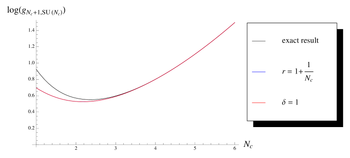
Figure 4: The case of $N_{f}=N_{c}+1$: The graphs of $\log g_{N_{c}+1,SU(N_{c})}(t,\widetilde{t})$ given by (3.2.4) with its asymptotic formulae (3.193) and (3.200). We take $\delta=1$, $r=1+1/N_{c}$, $t=0.3$ and $\widetilde{t}=0.1$. Note that the graphs for both asymptotic formulae are on top of each other in this figure.

In Figure 5, we plot the graphs of $\log g_{N_{c}+5,SU(N_{c})}(t,\widetilde{t})$ given by the asymptotic formulae (3.193) and (3.200) against $N_{c}$, with $\delta=5$, $r=1+5/N_{c}$, $t=0.3$ and $\widetilde{t}=0.1$. It can be see that the asymptotic formula (3.193) approaches the asymptotic formula (3.200) for large $N_{c}$.

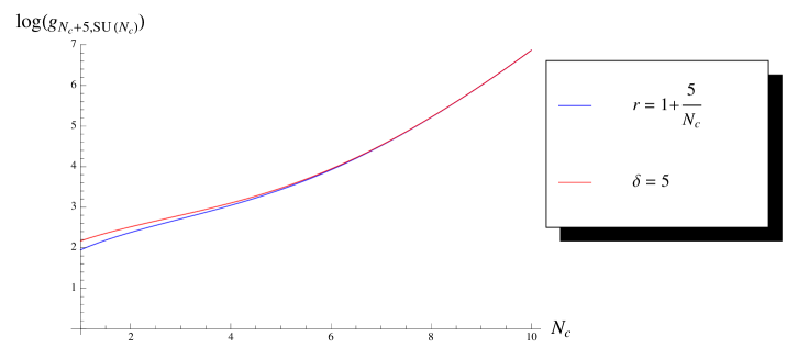
Figure 5: The case of $N_{f}=N_{c}+5$: The graphs of $\log g_{N_{c}+5,SU(N_{c})}(t,\widetilde{t})$ given by the asymptotic formulae (3.193) and (3.200). We take $\delta=5$, $r=1+5/N_{c}$, $t=0.3$ and $\widetilde{t}=0.1$.

Let us now set $t=\widetilde{t}$. In Figure 6, we plot the graphs of $\log g_{6,SU(3)}(t,t)$ given by (3.3) and (3.200) (with $r=2$ and $N_{c}=3$) against $t$. As we expected from the second limiting case in §2.6.2, the asymptotic formula should give a good approximation when $t=O(N_{c}^{-1/2})$. Indeed, as one can see from the graph, the asymptotic result is in agreement with the exact result for $t<1/\sqrt{N_{c}}=1/\sqrt{3}\approx 0.58$.

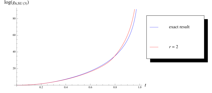
Figure 6: The case of $N_{c}=3,N_{f}=6$ and $t=\widetilde{t}$: The graphs of $\log g_{6,SU(3)}(t,t)$ from (3.3) and its asymptotic formula (3.200) (with $r=2$ and $N_{c}=3$). As we expected from the second limiting case in §2.6.2, the asymptotic formula is in agreement with the exact result for $t<1/\sqrt{N_{c}}=1/\sqrt{3}\approx 0.58$.

Appendix A Multi-contour integrals and determinants

In this section, we show that one can rewrite the contour integrals in the Hilbert series of $U(N_{c})$ SQCD in terms of a determinant. A key tool is Gram’s formula (see, e.g., Appendix A.12 of mehta ), which states as follows. Let

$$b_{ij}=\sum_{\alpha=1}^{n}v_{i\alpha}v^{*}_{j\alpha}~{},\quad i,j=1,2,\ldots,m~{};$$ (A.201)

then

$$\frac{1}{m!}\sum_{\alpha_{1}=1}^{n}\cdots\sum_{\alpha_{m}=1}^{n}\left|\det(v_{i\alpha_{j}})_{1\leq i,j\leq m}\right|^{2}=\det(b_{ij})_{1\leq i,j\leq m}~{}.$$ (A.202)

The $U(N_{c})$ Haar measure.

Let us first consider the $U(N_{c})$ Haar measure

$$\int\mathrm{d}\mu_{U(N_{c})} = \frac{1}{N_{c}!(2\pi i)^{N_{c}}}\oint_{|z_{1}|=1}\frac{\mathrm{d}z_{1}}{z_{1}}\cdots\oint_{|z_{N_{c}}|=1}\frac{\mathrm{d}z_{N_{c}}}{z_{N_{c}}}|\Delta_{N_{c}}(z)|^{2}$$ (A.203)

$$= \frac{1}{N_{c}!(2\pi i)^{N_{c}}}\oint_{|z_{1}|=1}\frac{\mathrm{d}z_{1}}{z_{1}}\cdots\oint_{|z_{N_{c}}|=1}\frac{\mathrm{d}z_{N_{c}}}{z_{N_{c}}}\left|\det(z_{a}^{b-1})_{1\leq a,b\leq N_{c}}\right|^{2}~{}.$$

Let us now apply (A.202). We take $m=N_{c}$ and make the following substitutions:

$$\sum_{\alpha=1}^{n}\quad \longrightarrow \quad\frac{1}{2\pi i}\oint_{|z|=1}\frac{\mathrm{d}z}{z}$$

$$\sum_{\alpha_{1}=1}^{n}\cdots\sum_{\alpha_{m}=1}^{n}\quad \longrightarrow \quad\frac{1}{(2\pi i)^{N_{c}}}\oint_{|z_{1}|=1}\frac{\mathrm{d}z_{1}}{z_{1}}\cdots\oint_{|z_{N_{c}}|=1}\frac{\mathrm{d}z_{N_{c}}}{z_{N_{c}}}~{},$$

$$v_{i\alpha_{j}}\quad \longrightarrow \quad z_{a}^{b-1}~{}.$$ (A.204)

Thus, from (A.201), we find that

$$b_{ab}=\frac{1}{2\pi i}\oint_{|z|=1}\frac{\mathrm{d}z}{z}z^{a-1}(z^{b-1})^{*}=\frac{1}{2\pi i}\oint_{|z|=1}\frac{\mathrm{d}z}{z}z^{a-1}z^{1-b}=\frac{1}{2\pi i}\oint_{|z|=1}\frac{\mathrm{d}z}{z}z^{a-b}~{}.$$ (A.205)

Thus, from (A.202), (A.203) and (A.205), we can rewrite the Haar measure of $U(N_{c})$ as

$$\int\mathrm{d}\mu_{U(N_{c})}=\det\left(\frac{1}{2\pi i}\oint_{|z|=1}\frac{\mathrm{d}z}{z}z^{a-b}\right)_{1\leq a,b\leq N_{c}}~{}.$$ (A.206)

The $U(N_{c})$ SQCD Hilbert series.

Now consider the integral of the type:

$$\mathcal{I}(\xi)=\int\mathrm{d}\mu_{U(N_{c})(z_{1},\ldots,z_{N_{c}})}\prod_{a=1}^{N_{c}}\phi(\xi,z_{a})~{}.$$ (A.207)

Note that this is also the integral we encounter in (2.37) in the context of $U(N_{c})$ SQCD. We make a similar substitution as in (A.204):

$$\sum_{\alpha=1}^{n}\quad \longrightarrow \quad\frac{1}{2\pi i}\oint_{|z|=1}\frac{\mathrm{d}z}{z}\phi(\xi,z)~{},$$

$$\sum_{\alpha_{1}=1}^{n}\cdots\sum_{\alpha_{m}=1}^{n}\quad \longrightarrow \quad\frac{1}{(2\pi i)^{N_{c}}}\oint_{|z_{1}|=1}\frac{\mathrm{d}z_{1}}{z_{1}}\cdots\oint_{|z_{N_{c}}|=1}\frac{\mathrm{d}z_{N_{c}}}{z_{N_{c}}}\prod_{a=1}^{N_{c}}\phi(\xi,z_{a})~{},$$

$$v_{i\alpha_{j}}\quad \longrightarrow \quad z_{a}^{b-1}~{}.$$ (A.208)

Thus, from (A.202), we find that

$$\mathcal{I}(\xi)=\det\left(\frac{1}{2\pi i}\oint_{|z|=1}\frac{\mathrm{d}z}{z}z^{a-b}\phi(\xi,z)\right)_{1\leq a,b\leq N_{c}}~{}.$$ (A.209)

Appendix B A delta function in the contour integral

Let $f(z)$ a function which is analytic everywhere on the unit circle. In this section, we show that the delta function in the integral

$$\oint_{|z|=1}\frac{\mathrm{d}z}{z}\delta(z-1)f(z)$$ (B.210)

can be replaced by an infinite sum as

$$\delta(z-1)\rightarrow\frac{1}{2\pi i}\sum_{k=-\infty}^{\infty}z^{k}~{},$$ (B.211)

so that we have

$$\oint_{|z|=1}\frac{\mathrm{d}z}{z}\delta(z-1)f(z)=\frac{1}{2\pi i}\sum_{k=-\infty}^{\infty}\oint_{|z|=1}\frac{\mathrm{d}z}{z}z^{k}f(z)~{}.$$ (B.212)

Proof.

Consider

$$f(1)=\oint_{|z|=1}\frac{\mathrm{d}z}{z}\delta(z-1)f(z)=i\int_{-\pi}^{\pi}\mathrm{d}\theta~{}\delta(e^{i\theta}-1)f(e^{i\theta})~{}.$$ (B.213)

Note that

$$\delta(e^{i\theta}-1)=-i\sum_{n=-\infty}^{\infty}\delta(\theta-2\pi n)=-\frac{i}{2\pi}\sum_{k=-\infty}^{\infty}e^{ik\theta}~{},$$ (B.214)

where the first equality can be verified by integrating from $2\pi m-\pi$ to $2\pi m+\pi$ (for any $m\in\mathbb{Z}$) and noting that $-i=\int_{-\pi}^{\pi}\mathrm{d}\theta~{}\delta(e^{i\theta}-1)$, whereas in the last step we have used the Poisson summation formula. Substituting this back into (B.213), we obtain

$$\oint_{|z|=1}\frac{\mathrm{d}z}{z}\delta(z-1)f(z)=\frac{1}{2\pi}\sum_{k=-\infty}^{\infty}\int_{-\pi}^{\pi}\mathrm{d}\theta~{}e^{ik\theta}f(e^{i\theta})~{}.$$ (B.215)

Writing $z=e^{i\theta}$ on the right hand side, we arrive at

$$\oint_{|z|=1}\frac{\mathrm{d}z}{z}\delta(z-1)f(z)=\frac{1}{2\pi i}\sum_{k=-\infty}^{\infty}\oint_{|z|=1}\frac{\mathrm{d}z}{z}z^{k}f(z)~{}.$$ (B.216)

This amounts to the replacement

$$\delta(z-1)\rightarrow\frac{1}{2\pi i}\sum_{k=-\infty}^{\infty}z^{k}~{}.$$ (B.217)

References

- (1) D. Forcella, “Master Space and Hilbert Series for Field Theories,” arXiv:0902.2109 [hep-th].
- (2) A. Hanany, “Counting BPS Operators in the Chiral Ring: the Plethystic Story,” AIP Conf. Proc. 939 (2007) 165.
- (3) S. Benvenuti, B. Feng, A. Hanany and Y. H. He, “Counting BPS Operators in Gauge Theories: Quivers, Syzygies and Plethystics,” JHEP 0711 (2007) 050 [arXiv:hep-th/0608050].
- (4) B. Feng, A. Hanany and Y. H. He, “Counting Gauge Invariants: the Plethystic Program,” JHEP 0703 (2007) 090 [arXiv:hep-th/0701063].
- (5) D. Forcella, A. Hanany, Y. H. He and A. Zaffaroni, “The Master Space of Gauge Theories,” JHEP 0808 (2008) 012 [arXiv:0801.1585 [hep-th]].
- (6) D. Forcella, A. Hanany and A. Zaffaroni, “Master Space, Hilbert Series and Seiberg Duality,” JHEP 0907 (2009) 018 [arXiv:0810.4519 [hep-th]].
- (7) P. Pouliot, “Molien Function for Duality,” JHEP 9901 (1999) 021 [arXiv:hep-th/9812015].
- (8) C. Römelsberger, “Counting Chiral Primaries in , Superconformal Field Theories,” Nucl. Phys. B 747 (2006) 329 [arXiv:hep-th/0510060].
- (9) J. Gray, A. Hanany, Y. H. He, V. Jejjala and N. Mekareeya, “SQCD: a Geometric Aperçu,” JHEP 0805 (2008) 099 [arXiv:0803.4257 [hep-th]].
- (10) A. Hanany and N. Mekareeya, “Counting Gauge Invariant Operators in SQCD with Classical Gauge Groups,” JHEP 0810 (2008) 012 [arXiv:0805.3728 [hep-th]].
- (11) D. Forcella, A. Hanany and A. Zaffaroni, “Baryonic Generating Functions,” JHEP 0712 (2007) 022 [arXiv:hep-th/0701236].
- (12) A. Butti, D. Forcella, A. Hanany, D. Vegh and A. Zaffaroni, “Counting Chiral Operators in Quiver Gauge Theories,” JHEP 0711 (2007) 092 [arXiv:0705.2771 [hep-th]].
- (13) F. A. Dolan, “Counting BPS Operators in SYM,” Nucl. Phys. B 790 (2008) 432 [arXiv:0704.1038 [hep-th]].
- (14) A. Hanany, N. Mekareeya and G. Torri, “The Hilbert Series of Adjoint SQCD,” Nucl. Phys. B 825 (2010) 52 [arXiv:0812.2315 [hep-th]].
- (15) A. Hanany, N. Mekareeya and A. Zaffaroni, “Partition Functions for Membrane Theories,” JHEP 0809 (2008) 090 [arXiv:0806.4212 [hep-th]].
- (16) A. Hanany, D. Vegh and A. Zaffaroni, “Brane Tilings and M2 Branes,” JHEP 0903 (2009) 012 [arXiv:0809.1440 [hep-th]].
- (17) J. Davey, A. Hanany, N. Mekareeya and G. Torri, “Phases of M2-Brane Theories,” JHEP 0906 (2009) 025 [arXiv:0903.3234 [hep-th]].
- (18) J. Davey, A. Hanany, N. Mekareeya and G. Torri, “Higgsing M2-Brane Theories,” JHEP 0911 (2009) 028 [arXiv:0908.4033 [hep-th]].
- (19) J. Davey, A. Hanany, N. Mekareeya and G. Torri, “M2-Branes and Fano 3-Folds,” arXiv:1103.0553 [hep-th].
- (20) A. Hanany, D. Forcella and J. Troost, “The Covariant Perturbative String Spectrum,” Nucl. Phys. B 846 (2011) 212 [arXiv:1007.2622 [hep-th]].
- (21) H. Nakajima and K. Yoshioka, “Instanton Counting on Blowup. I,” arXiv:math/0306198.
- (22) S. Benvenuti, A. Hanany and N. Mekareeya, “The Hilbert Series of the One Instanton Moduli Space,” JHEP 1006 (2010) 100 [arXiv:1005.3026 [hep-th]].
- (23) A. Hanany and C. Römelsberger, “Counting BPS Operators in the Chiral Ring of Supersymmetric Gauge Theories Or Braine Surgery,” Adv. Theor. Math. Phys. 11 (2007) 1091 [arXiv:hep-th/0611346].
- (24) A. Hanany and N. Mekareeya, “Tri-Vertices and ’s,” JHEP 1102 (2011) 069 [arXiv:1012.2119 [hep-th]].
- (25) N. Seiberg, “Exact results on the space of vacua of four-dimensional susy gauge theories,” Phys. Rev. D 49, 6857 (1994) [arXiv:hep-th/9402044].
- (26) K. A. Intriligator and N. Seiberg, “Phases of N=1 supersymmetric gauge theories in four dimensions,” Nucl. Phys. B 431, 551 (1994) [arXiv:hep-th/9408155].
- (27) N. Seiberg, “Electric - magnetic duality in supersymmetric nonAbelian gauge theories,” Nucl. Phys. B 435, 129 (1995) [arXiv:hep-th/9411149].
-
(28)
P. Argyres, “Introduction to supersymmetry,”
http://www.physics.uc.edu/~argyres/661/susy2001.pdf - (29) J. Terning, Modern supersymmetry: Dynamics and duality, Oxford, UK: Clarendon (2006).
- (30) K. Intriligator and N. Seiberg, “Lectures on supersymmetry breaking,” Class. Quant. Grav. 24, S741 (2007) [arXiv:hep-ph/0702069].
- (31) K. A. Intriligator and N. Seiberg, “Lectures on supersymmetric gauge theories and electric-magnetic duality,” Nucl. Phys. Proc. Suppl. 45BC, 1 (1996) [arXiv:hep-th/9509066].
- (32) I. Affleck, M. Dine, and N. Seiberg, Dynamical supersymmetry breaking in supersymmetric QCD,” Nucl. Phys. B 241, 493 (1984).
- (33) M. Shifman and A. Yung, “Confinement in SQCD: One Step Beyond Seiberg’s Duality,” Phys. Rev. D 76 (2007) 045005 [arXiv:0705.3811 [hep-th]].
- (34) A. Gorsky, M. Shifman and A. Yung, “ Supersymmetric Quantum Chromodynamics: How Confined Non-Abelian Monopoles Emerge from Quark Condensation,” Phys. Rev. D 75 (2007) 065032 [arXiv:hep-th/0701040].
- (35) H. Derksen and G. Kemper, “Computational Invariant Theory,” Springer-Verlag, New York (2002).
- (36) D. Z. Djokovic, “Poincare series of some pure and mixed trace algebras of two generic matrices,” arXiv:math.AC/0609262
- (37) W. Fulton and J. Harris Representation Theory: A First Course, New York: Springer (1991).
- (38) N. M. Katz and P. Sarnak Random Matrices, Frobenius Eigenvalues, and Monodromy, Rhode Island: American Mathematical Society (1998).
- (39) A. Böttcher and B. Silbermann, “Analysis of Toeplitz Operators,” Springer, Berlin (2006).
- (40) A. Böttcher and H. Widom, “Szegő via Jacobi,” Lin. Alg. Appl. 419 (2006) 656–667 [arXiv:math/0604009].
- (41) E. L. Basor and H. Widom, “On A Toeplitz Determinant Identity of Borodin and Okounkov,” Integral Equations and Operator Theory, 37, 397-401 (2000) [arXiv:math/9909010].
- (42) M. L. Mehta, “Random Matrices,” Elsevier (2004)
- (43) J. S. Geronimo and K. M. Case, “Scattering Theory and Polynomials Orthogonal on the Unit Circle,” J. Math. Phys. 20 (1979) 299.
- (44) A. Borodin and A. Okounkov, “A Fredholm determinant formula for Toeplitz determinants,” Integral Equations Operator Theory 37 (2000) 386–396. [arXiv:math/9907165]
- (45) G. Szegő, “On certain Hermitian forms associated with the Fourier series of a positive function,” in: Festschrift Marcel Riesz, Lund 1952, pp. 222–238.
- (46) M. E. Fisher and R. E. Hartwig, “Toeplitz determinants: some applications, theorems, and conjectures”, Adv. Chem. Phys. 15 (1968) 333–353.
- (47) M. E. Fisher and R. E. Hartwig, “Asymptotic behavior of Toeplitz matrices and determinants”, Arch. Ration. Mech. Anal. 32 (1969) 190–225.
- (48) A. Böttcher and B. Silbermann, “Notes on the asymptotic behavior of block Toeplitz matrices and determinants”, Math. Nachr. 98 (1980) 183–210.
- (49) C. A. Tracy and H. Widom, “On the distributions of the lengths of the longest monotone subsequences in random words”, Prob. Th. Rel. Fields 119 (2001) 350–380.
- (50) M. Mariño, “Les Houches Lectures on Matrix Models and Topological Strings,” arXiv:hep-th/0410165.
- (51) A. Kapustin, B. Willett and I. Yaakov, “Exact Results for Wilson Loops in Superconformal Chern-Simons Theories with Matter,” JHEP 1003 (2010) 089 [arXiv:0909.4559 [hep-th]].
- (52) M. Mariño and P. Putrov, “Exact Results in ABJM Theory from Topological Strings,” JHEP 1006 (2010) 011 [arXiv:0912.3074 [hep-th]].
- (53) D. Martelli and J. Sparks, “The Large Limit of Quiver Matrix Models and Sasaki-Einstein Manifolds,” arXiv:1102.5289 [hep-th].
- (54) S. Cheon, H. Kim and N. Kim, “Calculating the Partition Function of Gauge Theories on S3 and AdS/CFT Correspondence,” arXiv:1102.5565 [hep-th].
- (55) D. L. Jafferis, I. R. Klebanov, S. S. Pufu and B. R. Safdi, “Towards the F-Theorem: Field Theories on the Three-Sphere,” arXiv:1103.1181 [hep-th].
- (56) C. P. Herzog, I. R. Klebanov, S. S. Pufu and T. Tesileanu, “Multi-Matrix Models and Tri-Sasaki Einstein Spaces,” Phys. Rev. D 83 (2011) 046001 [arXiv:1011.5487 [hep-th]].
- (57) V. Balasubramanian, E. Keski-Vakkuri, P. Kraus and A. Naqvi, “String Scattering from Decaying Branes,” Commun. Math. Phys. 257 (2005) 363 [arXiv:hep-th/0404039].
- (58) N. Jokela, E. Keski-Vakkuri and J. Majumder, “On Superstring Disk Amplitudes in a Rolling Tachyon Background,” Phys. Rev. D 73 (2006) 046007 [arXiv:hep-th/0510205].
- (59) N. Jokela, M. Jarvinen and E. Keski-Vakkuri, “N-Point Functions in Rolling Tachyon Background,” Phys. Rev. D 79 (2009) 086013 [arXiv:0806.1491 [hep-th]].
- (60) N. Jokela, M. Jarvinen and E. Keski-Vakkuri, “Electrostatics Approach to Closed String Pair Production from a Decaying D-Brane,” Phys. Rev. D 80 (2009) 126010 [arXiv:0911.0339 [hep-th]].
- (61) N. Jokela, M. Jarvinen and E. Keski-Vakkuri, “Electrostatics of Coulomb Gas, Lattice Paths, and Discrete Polynuclear Growth,” J. Phys. A 43 (2010) 425006 [arXiv:1003.3663 [hep-th]].