Chiral polymerization: symmetry breaking and entropy production in closed systems

Abstract

We solve numerically a kinetic model of chiral polymerization in systems closed to matter and energy flow, paying special emphasis to its ability to amplify the small initial enantiomeric excesses due to the internal and unavoidable statistical fluctuations. The reaction steps are assumed to be reversible, implying a thermodynamic constraint among some of the rate constants. Absolute asymmetric synthesis is achieved in this scheme. The system can persist for long times in quasi-stationary chiral asymmetric states before racemizing. Strong inhibition leads to long-period chiral oscillations in the enantiomeric excesses of the longest homopolymer chains. We also calculate the entropy production $\sigma$ per unit volume and show that $\sigma$ increases to a peak value either before or in the vicinity of the chiral symmetry breaking transition.

I Introduction

There is a growing consensus that the homochirality of biological compounds is a condition associated to life that should have emerged in the abiotic stages of evolution through processes of spontaneous mirror symmetry breaking (SMSB). This could have proceeded in a prebiotic stage, incorporating steps of increasing complexity thus leading to chemical systems and enantioselective chemical networks AG ; Weissbuch ; Guijarro . An important issue is therefore to identify processes of chirality amplification in chemical reactions. In this regard, a recent kinetic analysis of the Frank model in closed systems applied to the Soai reaction CHMR has taught us that in an actual chemical scenario, reaction networks that exhibit SMSB are very sensitive to chiral inductions owing to the presence of tiny initial enantiomeric excesses, as previously shown theoretically KondeAvet . The stochastic scenario implies the creation of chirality from intrinsic chiral fluctuations and its later transmission and amplification. This can occur in far-from-equilibrium systems that undergo dynamic phase transitions.

The process must be coupled to others which preserve, extend, and transmit the chirality. Biological homochirality of living systems involves large macromolecules, therefore a central point is the relationship of the polymerization process with the emergence of chirality. This hypothesis has inspired recent activity devoted to modeling efforts aimed at understanding mirror symmetry breaking in polymerization of relevance to the origin of life. The models so proposed Sandars ; BM ; BAHN ; WC ; Gleisera ; Gleiserb ; Gleiserc ; Gleiserd ; SH are by and large, elaborate extensions and generalizations of Frank’s original paradigmatic scheme Frank . Heading this list, Sandars Sandars introduced a detailed polymerization process plus the basic elements of enantiomeric cross inhibition as well as a chiral feedback mechanism in which only the largest polymers formed can enhance the production of the monomers from an achiral substrate. He treated basic numerical studies of symmetry breaking and bifurcation properties of this model for various values of the number of repeat units $N$. All the subsequent models cited here are variations on Sandars’ original theme. Soon afterwards, Brandenburg and coworkers BAHN studied the stability and conservation properties of a modified Sandars’ model and introduce a reduced $N=2$ version including the effects of chiral bias. In BM , they included spatial extent in this model to study the spread and propagation of chiral domains as well as the influence of a backround turbulent advection velocity field. The model of Wattis and Coveney WC differs from Sandars’ in that they allow for polymers to grow to arbitrary lengths $N$ and the chiral polymers of all lengths, from the dimer and upwards, act catalytically in the breakdown of the achiral source into chiral monomers. An analytic linear stability analysis of both the racemic and chiral solutions is carried out for the model’s large $N$ limit and various kinetic timescales are identified. The role of external white noise on Sandars-type polymerization networks including spatial extent has been explored by Gleiser and coworkers: the $N=2$ truncated model introduced in BM is subjected to external white noise in Gleisera , chiral bias is considered in Gleiserb , high intensity and long duration noise is considered in Gleiserc and in Gleiserd , modified Sandars-type models with spatial extent and external noise are considered both for finite and infinite $N$, with an emphasis paid to the dynamics of chiral symmetry breaking. By contrast, Saito and Hyuga’s SH model gives rise to homochiral states but differs markedly from Sandars’ in that it does not invoke the enantiomeric cross inhibition, allowing instead for reversibility in all the reaction steps. Their model requires open flow, which is the needed element of irreversibility. A different model which stands apart from the above group is that due to Plasson et al. Plasson . They considered a recycled system based on reversible chemical reactions and open only to energy flow and without any (auto)catalytic reactions. A source of constant external energy –the element of irreversibility–is required to activate the monomers. This energy could be introduced into the system in a physical form, say, as high energy photons. A system of this kind, limited to dimerizations, was shown to have nonracemic stable final states for various ranges of the model parameter values and for total concentrations greater than a minimal value.

The polymerization models referred to above are defined only for open flow systems which exchange matter and energy with the exterior. A constant source of achiral precursor is usually assumed. An unrealistic consequence is that homochiral chains can grow to infinite length. By contrast, most experimental procedures are carried out in closed and spatially bounded reaction domains and are initiated in far-from equilibrium states Blocher ; Weissbuch ; Hitzb ; Nery ; Hitza ; Rubinstein ; Illos ; Lahava ; Lahavb . It is thus crucial to have models compatible with these experimentally realistic boundary and initial conditions. The most immediate consequences are that polymer chains can grow to a finite maximum length and that the total system mass is constant. These two properties are of course intimately related. An original aspect of our work is that we consider the polymerization process in a closed system and include reversible reactions. This enables us to explore absolute asymmetric synthesis in thermodynamically closed systems (closed to matter flow) taking into account the backward reaction steps, which we call here ”reversible reactions/reversible models” in spite of the fact that the values of the forward and reverse rate constants can be very different. As we are eloquently reminded by Mislow, mirror asymmetric states are in practice unavoidable on purely statistical grounds alone Mislow , even in the absence of chiral physical forces. Absolute asymmetric synthesis is the ability of a system to amplify these statistical and minuscule enantiomeric biases up to observably large excesses. Thus a major goal of this work is assess the ability of such polymerization schemes to amplify these initial excesses, albeit if only temporarily. Asymmetric amplification is demonstrated to occur obeying microscopic reversibility in a reversible model closed to matter flow. This is of great practical interest as the racemization time scale can be substantially longer than that of the transformation of the initial reagents, depending on the strength of the mutual inhibition, or direct interaction between the enantiomers. And regarding chemical evolution, this obviates the need to invoke chiral physical fields and lends further support to the conviction that homochirality is a “stereochemical imperative” of molecular evolution Siegel .

The behavior of entropy in polymerization models is rarely discussed Stier , and has not been addressed for mirror symmetry breaking in chiral polymerization. The entropy produced in a chemical reaction initiated out of equilibrium gives a measure of the dissipation during the approach to final equilibrium. In this paper, we calculate the rate of entropy production in chiral polymerization. Depending on the enantiomeric mutual inhibition, the entropy production undergoes a rapid increase to a peak value either before, or else in the vicinity of the chiral symmetry breaking transition, followed by an equally dramatic decrease. The system racemizes at time scales greater than that of polymerization, and is accompanied by a final decrease of entropy production to zero, indicating that the system has reached a final stable state (not to be confused with a stationary state, which must be accompanied by a nonzero constant entropy production). Computation of the average length homopolymer indicates that the final racemic state is dominated by the longest available chains.

II The polymerization model

The model we introduce and study here is modified and extended from that of Wattis and Coveney WC which is in turn, a generalization of Sandar’s scheme Sandars . Two salient differences that distinguish our model from these and other previous ones Sandars ; BM ; BAHN ; WC ; Gleisera ; Gleiserb ; Gleiserc ; Gleiserd ; SH are that we (1) consider polymerization in closed systems Hoch –, so that no matter flow is permitted with an external environment– and (2) we allow for reversible reactions in all the steps. A third difference is that we also include the formation (and dissociation) of the heterodimer. While heterodimer formation was originally contemplated in Sandars , it has been silently omitted from all the subsequent models BM ; BAHN ; WC ; Gleisera ; Gleiserb ; Gleiserc ; Gleiserd that derive therefrom. Fragmentation in a Sandars type model has been considered previously, but was shown to yield a maximum average polymer length of only $N=3$ repeat units BAN .

We assume there is an achiral precursor $S$ which can directly produce the chiral monomers $L_{1}$ and $R_{1}$ at a slow rate $\epsilon$ as well as be consumed in processes in which homopolymers of all lengths catalyze the production of monomers. The specific reaction scheme we study here is composed of the following steps, where the $\epsilon$, ($\epsilon_{-}$), $k$ ($k_{-}$), etc., denote the forward (reverse) reaction rate constants and $0\leq f\leq 1$ is the fidelity of the feedback mechanism:

$$\begin{array}[]{ccc}S\stackrel{{\scriptstyle\epsilon}}{{\rightleftharpoons\atop{\small\epsilon_{-}}}}L_{1},&S+Q\stackrel{{\scriptstyle\frac{k}{2}(1+f)}}{{\rightleftharpoons\atop{\small\frac{k_{-}}{2}(1+f)}}}L_{1}+Q,&S+P\stackrel{{\scriptstyle\frac{k}{2}(1-f)}}{{\rightleftharpoons\atop{\small\frac{k_{-}}{2}(1-f)}}}L_{1}+P\\ \\ S\stackrel{{\scriptstyle\epsilon}}{{\rightleftharpoons\atop{\small\epsilon_{-}}}}R_{1},&S+P\stackrel{{\scriptstyle\frac{k}{2}(1+f)}}{{\rightleftharpoons\atop{\small\frac{k_{-}}{2}(1+f)}}}R_{1}+P,&S+Q\stackrel{{\scriptstyle\frac{k}{2}(1-f)}}{{\rightleftharpoons\atop{\small\frac{k_{-}}{2}(1-f)}}}R_{1}+Q.\end{array}$$ (1)

Here

$$Q=\sum_{n=1}^{N}nL_{n},\qquad P=\sum_{n=1}^{N}nR_{n},$$ (2)

represent a measure of the total concentrations of left-handed and right handed polymers. The amount of each chiral monomer produced is influenced by the total amount of chiral oligomer already present in the system. We allow for the monomers themselves to participate in these substrate reactions: hence $N\geq n\geq 1$, where $N$ is the maximum chain length. The central top and bottom reactions in Eq. (1) are enantioselective, whereas those on the right hand side are non-enantioselective. The model therefore contains the features of limited enantioselectivity, first proposed as an alternative to the mutual inhibition of Frank AG .

An important observation is that differences in the Gibbs free energy $\Delta G^{0}$ between initial and final states should be the same in all the reactions listed in Eq.(1), which implies the thermodynamic constraint on the following forward and reverse reaction constants (see also SH )

$$\frac{\epsilon}{\epsilon_{-}}=\frac{k}{k_{-}}.$$ (3)

The polymerization and chain end-termination reactions (see below) are not subject to a thermodynamic constraint.

The monomers combine to form chirally pure polymer chains denoted by $L_{n}$ and $R_{n}$, according to the isodesmic Meijer stepwise reactions for $1\leq n\leq N-1$

$$\begin{array}[]{cc}L_{n}+L_{1}\stackrel{{\scriptstyle k_{aa}}}{{\rightleftharpoons\atop{\small k^{-}_{aa}}}}L_{n+1},&R_{n}+R_{1}\stackrel{{\scriptstyle k_{bb}}}{{\rightleftharpoons\atop{\small k^{-}_{bb}}}}R_{n+1},\end{array}$$ (4)

and inhibition, or the chain end-termination reactions for $N-1\geq n\geq 2$:

$$\begin{array}[]{cc}L_{n}+R_{1}\stackrel{{\scriptstyle k_{ab}}}{{\rightleftharpoons\atop{\small k^{-}_{ab}}}}RL_{n},&R_{n}+L_{1}\stackrel{{\scriptstyle k_{ba}}}{{\rightleftharpoons\atop{\small k^{-}_{ba}}}}LR_{n}.\end{array}$$ (5)

These upper limits for $n$ specified in Eqs.(4,5) ensure that the maximum length for all oligomers produced (or consumed) by these reaction sets, both the homo- and heterochiral ones, is never greater than $N$. In the remainder of this paper we will consider here the natural and chiral symmetric rate assignments $k_{aa}=k_{bb}$, $k_{ab}=k_{ba}$ and likewise for the inverse rates, $k^{-}_{aa}=k^{-}_{bb}$ and $k^{-}_{ab}=k^{-}_{ba}$. There are then four independent rate constants.

We include a separate reaction for the heterodimer formation and dissociation:

$$L_{1}+R_{1}\stackrel{{\scriptstyle k_{h}}}{{\rightleftharpoons\atop{\small k^{-}_{h}}}}H\equiv L_{1}R_{1},$$ (6)

where $k_{h}=(k_{ab}+k_{ba})/2$ and $k^{-}_{h}=(k^{-}_{ab}+k^{-}_{ba})/2$. Note that these latter two rate constants are automatically determined from the above choice and that $L_{1}R_{1}=R_{1}L_{1}$ of course. This completes the specification of the model’s reactions.

The model is left-right symmetric, that is, possesses a discrete $Z_{2}$ symmetry Chaikin , which is manifest in the elementary reaction steps, in the rate constants, and in the corresponding differential rate equations (see below). This symmetry can be broken spontaneously by the dynamical solutions of the differential rate equations. This model is thus apt for investigating spontaneous mirror symmetry breaking. Though not considered here, the effects of explicit chiral bias (e.g., that induced by external physical fields) can also be studied with this model by lifting the $Z_{2}$ degeneracy in the reaction rates, e.g., allowing for $k_{aa}\neq k_{bb}$, etc., leading to a maximum of eight independent rate constants for describing the reaction set in Eqs. (4,5).

Rate-equation theory as employed in chemical kinetics is used to describe the differential rate equations of the achiral source, the monomers, as well as the homo- and heterochiral oligomers belonging to this reaction network. The kinetic equations for the concentrations that follow from these elementary steps are as follows. We begin with the rate equations for the achiral precursor $S$ and those corresponding to the two chiral monomers:

$$\frac{d[S]}{dt} = -2\epsilon[S]-k[S](P+Q)+\epsilon_{-}([L_{1}]+[R_{1}])+\frac{1}{2}k_{-}[L_{1}]\big{(}(1+f)Q+(1-f)P\big{)}$$ (7)

$$+ \frac{1}{2}k_{-}[R_{1}]\big{(}(1+f)P+(1-f)Q\big{)},$$

$$\frac{d[L_{1}]}{dt} = \epsilon[S]+\frac{k}{2}[S]\big{(}(1+f)Q+(1-f)P\big{)}-k_{aa}[L_{1}]\Big{(}2[L_{1}]+\sum_{n=2}^{N-1}[L_{n}]+k_{ba}/k_{aa}\sum_{n=1}^{N-1}[R_{n}]\Big{)}$$ (8)

$$- \epsilon_{-}[L_{1}]-\frac{k_{-}}{2}[L_{1}]\big{(}(1+f)Q+(1-f)P\big{)}$$

$$+ k_{aa}^{-}\Big{(}2[L_{2}]+\sum_{n=2}^{N-1}[L_{n+1}]+k_{ba}^{-}/k_{aa}^{-}\sum_{n=2}^{N-1}[LR_{n}]\Big{)}+k_{h}^{-}H,$$

$$\frac{d[R_{1}]}{dt} = \epsilon[S]+\frac{k}{2}[S]\big{(}(1+f)P+(1-f)Q\big{)}-k_{bb}[R_{1}]\Big{(}2[R_{1}]+\sum_{n=2}^{N-1}[R_{n}]+k_{ab}/k_{bb}\sum_{n=1}^{N-1}[L_{n}]\Big{)}$$ (9)

$$- \epsilon_{-}[R_{1}]-\frac{k_{-}}{2}[R_{1}]\big{(}(1+f)P+(1-f)Q\big{)}$$

$$+ k_{bb}^{-}\Big{(}2[R_{2}]+\sum_{n=2}^{N-1}[R_{n+1}]+k_{ab}^{-}/k_{bb}^{-}\sum_{n=2}^{N-1}[RL_{n}]\Big{)}+k_{h}^{-}H.$$

Whereas for $N-1\geq n\geq 2$ we have the set of stepwise polymerization rate equations

$$\frac{d[L_{n}]}{dt} = k_{aa}[L_{1}]([L_{n-1}]-[L_{n}])-k_{ab}[L_{n}][R_{1}]+k_{ab}^{-}[RL_{n}]+k_{aa}^{-}([L_{n+1}]-[L_{n}]),$$ (10)

$$\frac{d[R_{n}]}{dt} = k_{bb}[R_{1}]([R_{n-1}]-[R_{n}])-k_{ba}[R_{n}][L_{1}]+k_{ba}^{-}[LR_{n}]+k_{bb}^{-}([R_{n+1}]-[R_{n}]).$$ (11)

Note, in accord with Eqs.(4,5) for the largest polymers $n=N$, we have instead the final pair

$$\frac{d[L_{N}]}{dt} = k_{aa}[L_{1}][L_{N-1}]-k_{aa}^{-}[L_{N}],$$ (12)

$$\frac{d[R_{N}]}{dt} = k_{bb}[R_{1}][R_{N-1}]-k_{bb}^{-}[R_{N}].$$ (13)

Then the kinetic equation for the heterodimer $H\equiv L_{1}R_{1}$ (which we keep separate from the other end-chain rate equations):

$$\frac{d[H]}{dt}=k_{h}[L_{1}][R_{1}]-k_{h}^{-}[H].$$ (14)

Lastly, for $N-1\geq n\geq 2$ the rate equations for the “end-spoiled” chains:

$$\frac{d[LR_{n}]}{dt} = k_{ba}[L_{1}][R_{n}]-k_{ba}^{-}[LR_{n}],$$ (15)

$$\frac{d[RL_{n}]}{dt} = k_{ab}[R_{1}][L_{n}]-k_{ab}^{-}[RL_{n}].$$ (16)

For chemical systems closed to matter flow, the constant mass constraint that must be obeyed by the coupled system of differential equations at every instant is given by (the overdot denotes time derivative):

$$[\dot{S}] + 2[\dot{H}]+\sum_{n=1}^{N}n([\dot{L}_{n}]+[\dot{R}_{n}])+\sum_{n=2}^{N-1}(n+1)\big{(}[\dot{R}L_{n}]+[\dot{L}R_{n}]\big{)}=0.$$ (17)

This relation can be verified directly using the above set of $4N-2$ kinetic equations Eqs. (7-16).

III Entropy production

The entropy production rate in an irreversible process is a measure of the dissipation in that process. At equilibrium, the entropy production rate vanishes and is an extremum RossVlad . This production has been investigated recently for reversible versions of the Frank model KondeKapcha ; Mauksch . In those simple models, the behavior of the entropy produced near the chiral symmetry breaking transition as well as its subsequent temporal development, depends on whether the chemical system is open or closed to matter flow. We will return to this important point below. Here we consider the behavior of the entropy produced by polymerization reactions and monomer catalysis when the system undergoes a chiral phase transition as well at the later stages when the system reaches final chemical equilibrium upon racemization.

For reactions obeying mass action kinetics, the entropy produced in any chemical reaction can be calculated straightforwardly in terms of the individual elementary reaction rates PrigoKonde ; RossVlad . The rate of entropy production is the sum over the difference of the forward ($R_{jf}$) and reverse ($R_{jr}$) reaction rates multiplied by the natural logarithm of the ratio of the forward and reverse rates PrigoKonde :

$$\sigma(t)=R^{*}\sum_{j}(R_{jf}-R_{jr})\ln\Big{(}\frac{R_{jf}}{R_{jr}}\Big{)}\geq 0,$$ (18)

where the sum runs over each elementary reaction step $j$, and $R^{*}=8.314\,{\rm J\,mol^{-1}\,K^{-1}}$ is the gas constant. Since our reaction scheme is set up for closed systems, equilibrium is reached after a racemization time scale $t_{racem}$ is reached, which suggests a further measure is provided by the total net entropy produced from the start of the reactions through chiral symmetry breaking, then on to final racemization, when the system reaches chemical and thermodynamic equilibrium and $\sigma(t>t_{racem})=0$

$$\sigma_{T}=\int_{0}^{t_{racem}}\sigma(u)\,du.$$ (19)

This quantifies the total dissipation over the complete history of the chemical transformations under study.

The sum in Eq.(18) contains $2N+4$ terms. In order to determine which specific steps of the full reaction network provide the leading contributions to $\sigma$, we group the forward and reverse reaction rates as follows:

III.1 Direct monomer production

$$R_{1f}=\epsilon[S] R_{1r}=\epsilon_{-}[L_{1}],$$ (20)

$$R_{2f}=\epsilon[S] R_{2r}=\epsilon_{-}[R_{1}].$$ (21)

III.2 Monomer catalysis

$$R_{3f}=\frac{k}{2}(1+f)[S][Q] R_{3r}=\frac{k_{-}}{2}(1+f)[L_{1}][Q],$$ (22)

$$R_{4f}=\frac{k}{2}(1+f)[S][P] R_{4r}=\frac{k_{-}}{2}(1+f)[R_{1}][P],$$ (23)

$$R_{5f}=\frac{k}{2}(1-f)[S][P] R_{5r}=\frac{k_{-}}{2}(1-f)[L_{1}][P],$$ (24)

$$R_{6f}=\frac{k}{2}(1-f)[S][Q] R_{6r}=\frac{k_{-}}{2}(1-f)[R_{1}][Q].$$ (25)

III.3 Polymerization

For $1\leq n\leq N-1$ we have

$$R_{nf}^{L}=k_{aa}[L_{1}][L_{n}] R_{nr}^{L}=k_{aa}^{-}[L_{n+1}],$$ (26)

$$R_{nf}^{R}=k_{bb}[R_{1}][R_{n}] R_{nr}^{R}=k_{bb}^{-}[R_{n+1}].$$ (27)

III.4 End-chain termination and the heterodimer

The heterodimer rates are

$$R^{h}_{f}=k_{h}[L_{1}][R_{1}]\qquad R^{h}_{r}=k_{h}^{-}[H],$$ (28)

whereas for $2\leq n\leq N-1$ the end-chain forward and reverse rates are given by

$$R_{nf}^{eR}=k_{ab}[L_{n}][R_{1}] R_{nr}^{eR}=k_{ab}^{-}[RL_{n}],$$ (29)

$$R_{nf}^{eL}=k_{ba}[R_{n}][L_{1}] R_{nr}^{eL}=k_{ba}^{-}[LR_{n}].$$ (30)

IV Results

As discussed in the Introduction, we are interested in testing the model’s ability to amplify the initial small statistical deviations about the idealized racemic composition Mislow , in systems closed to matter flow and taking microscopic reversibility fully into account. In order to study the sensitivity of the above reversible polymerization network to these minuscule initial enantiomeric excesses, a very dilute initial concentration of a scalemic (non racemic) mixture was employed in the calculations: the initial monomeric concentrations of $[L_{1}]_{0}=(1\times 10^{-6}+1\times 10^{-15})M$ and $[R_{1}]_{0}=1\times 10^{-6}M$ yielding an initial chiral excess of $ee_{0}=5\times 10^{-8}\%$. This is actually slightly lower Mills ; Mislow than the excess corresponding to the initial monomer concentrations ($ee_{0}=6.1\times 10^{-8}\%$). The initial concentration of the achiral substrate is $[S]_{0}=2M$, whereas those corresponding the homo- hetero-oligomers are all set to zero: $[L_{n}]_{0}=[R_{n}]_{0}=0$, for $2\leq n\leq N$, $[H]_{0}=0$, and $[LR_{n}]_{0}=[RL_{n}]_{0}=0$ for $2\leq n\leq N-1$. We choose $\epsilon=2\times 10^{-5}$, $\epsilon_{-}=10^{-10}$, $k=2.0$, $k_{-}=10^{-5}$, $f=0.9$, $k_{aa}=k_{bb}=1.0$, $k_{ab}=k_{ba}=10^{3}$, $k_{ab}^{-}=k_{ba}^{-}=1.0$, $k_{aa}^{-}=k_{bb}^{-}=10^{-5}$. For illustrative purposes, we consider chains that can grow to a maximum length of $N=12$. This $N$ value is intended as a mean “ball-park” figure suggested by recent experiments yielding homochiral chains anywhere from $N=5$ Hitzb up to $N=18$ Lahavb chiral repeat units, depending on the amino acids employed and the experimental conditions. The differential rate equations Eqs. (7-16) were numerically integrated with the version 7 Mathematica program package and using a level of numerical precision, typically twenty or more significant digits, to ensure the numerical significance of these initial concentrations and enantiomeric excess. The results were monitored and verified to assure that total system mass Eq. (17) remained constant in time.

Results are quantified in terms of a variety of convenient chiral measures. The percent enantiomeric excess values of the oligomers with homochiral sequence are calculated according to ($2\leq n\leq N)$

$$ee_{n}=\frac{[L_{n}]-[R_{n}]}{[L_{n}]+[R_{n}]}\times 100.$$ (31)

A global or ensemble-averaged measure of the degree of symmetry breaking is provided by the number-weighted enantiomeric excess $\eta$:

$$\eta=\frac{\sum_{n=2}^{N}([L_{n}]-[R_{n}])}{\sum_{n=2}^{N}([L_{n}]+[R_{n}])}\times 100.$$ (32)

The importance of the enantiomeric excess is that it provides the order parameter for the symmetry breaking transition: the $|ee|\geq 0$ is zero for chiral symmetric states and nonzero otherwise. In the latter case, the $Z_{2}$ symmetry is broken. The average chain length of the homopolymers is given by:

$${\bar{n}}=\frac{\sum_{n=2}^{N}n([L_{n}]+[R_{n}])}{\sum_{n=2}^{N}([L_{n}]+[R_{n}])},$$ (33)

and the root mean square deviation in the homochiral chain length are:

$$(\overline{n^{2}})^{1/2}\equiv\sqrt{<(n-{\bar{n}})^{2}>}=\sqrt{<n^{2}>-<n>^{2}}.$$ (34)

The angular brackets $<>$ denote averaging with respect to the ensemble $\sum_{n}([L_{n}]+[R_{n}])$, similar to Eq.(33). It is important to remember that these are all time-dependent quantities.

Temporary but rather long lived asymmetric amplification can take place, as shown in Figure 1; note the logarithmic time scale. The enantiomeric excess $\eta$ averaged over all chain lengths Eq. (32), from the dimer on up to the maximum length chain $N=12$ starts off at zero value until a time on the order of $t\sim 10$ at which the excess increases rapidly to nearly $100\%$ at SMSB. This is followed by a gradual stepwise decrease or chiral erosion characterized by the appearance of quasi-plateaus of approximate constancy: $\eta$ falls to about $90\%$ at $t\sim 10^{3}$, then to about $60\%$ at $t\sim 10^{6}$, staying approximately level until the final decrease to zero occurring at a time on the order of $t\sim 10^{11}-10^{12}$. The system has racemized on this time scale. No appreciable differences in $\eta$ can be discerned when we include the monomer, that is, start the sums at $n=1$: we still observe slow chiral erosion proceeding though quasi-steady plateaus. The rate of the entropy produced Eq. (18) exhibits an initial increase followed by a dramatic burst coinciding with the mirror symmetry breaking transition. This production then decreases rapidly to an exceedingly tiny but non zero value that remains constant during the entire period of slow chiral erosion, spanning more than ten orders of magnitude in time. The entropy production then goes strictly to zero when the system racemizes in complete accord with the fact that the system has reached chemical equilibrium. Although not displayed in Figure 1, the substrate concentration falls from its initial value to zero approximately coincident with the peak structure of the entropy production, thus suggesting a connection between the sharp production of the latter and the change in $S$. The total entropy produced Eq.(19) is $\sigma_{T}=378.4\,{\rm J\,mol^{-1}\,K^{-1}}$. We can identify the major contributions to the entropy production in this process, see Figure 2, from calculations of the partial entropies. In this way we find that the leading contribution comes from the monomer catalysis steps Eq.(1), followed by the polymerization itself Eq.(4), next by the mutual inhibition reactions: heterodimer formation Eq.(6) and the “end-spoiled” cross-inhibition reactions Eq.(5). The least important contribution comes from the direct production of monomers from the achiral substrate. The first three partial contributions all display a peak structure in the neighborhood of the symmetry breaking transition, with the corresponding peak values being displaced in time, see Figure 2. The exception to this is the entropy rate due to direct monomer production, which decreases monotonically.

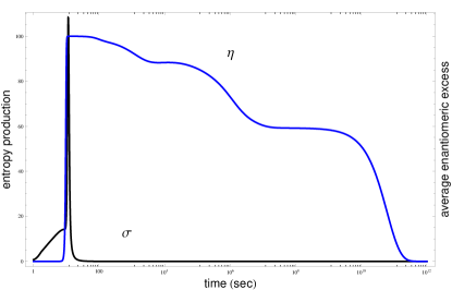
Figure 1: Time evolution (logarithmic time scale) of the average enantiomeric excess $\eta$, averaged over all chains ($2\leq n\leq 12$) Eq. (32), and the associated entropy production $\sigma$, Eq. (18). The entropy production peaks sharply at the onset of chiral symmetry breaking followed by a dramatic decrease to very small values. $\sigma$ strictly approaches zero only at the racemization time scale $t_{racem}\gtrsim 10^{11}$. Initial concentrations: $[L_{1}]_{0}=(1\times 10^{-6}+1\times 10^{-15})M$ and $[R_{1}]_{0}=1\times 10^{-6}M$ ($ee_{0}=5\times 10^{-8}\%$), $[S]_{0}=2M$, all other homo- and heterochiral oligomer initial concentrations are zero; and for the following rates $\epsilon=2\times 10^{-5}$, $\epsilon_{-}=10^{-10}$, $k=2.0$, $k_{-}=10^{-5}$, $f=0.9$, $k_{aa}=k_{bb}=1.0$, $k_{ab}=k_{ba}=10^{3}$, $k_{ab}^{-}=k_{ba}^{-}=1.0$, $k_{aa}^{-}=k_{bb}^{-}=10^{-5}$.

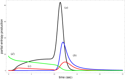
Figure 2: Partial contributions to the total entropy production. From, (a) limited enantioselective monomer catalysis, (b) stepwise polymerization reactions, (c) chain-end termination and heterodimer formation reactions $\times 20$, and (d) direct monomer production $\times 1000$. Note how the peak values of (a), (b) and (c) are displaced in time. Same initial concentrations and rate constants as in Fig. 1.

A finer or more detailed measure of the degree of symmetry breaking and amplification is provided by the individual percent chain-length dependent enantiomeric excesses, Eq.(31). A remarkable and complex dynamic behavior is revealed here. The time dependence of these $n$-dependent $ee$’s is plotted in Figure 3; note the logarithmic time scale. The individual $ee$’s follow a common curve from initialization to chiral symmetry breaking, at about $t\sim 10$, and remain together at nearly $100\%$ until about $t\sim 100$ at which time the common curve begins to split up into its constituents. Then, the percent chiral excess of each length homochiral chain behaves differently, until they again coalesce into a single curve upon final racemization, occurring at around $t\sim 10^{11}$. There is a common tendency for all the $ee$’s to decrease at intermediate time scales, with the largest length chains (here, $N=7,8,9,10,11,12$) passing from positive then to negative values of the excess. The $N=12,11,10$ chains exhibit nearly $-100\%$ excess during the period from $10^{3}$ to $10^{4}$ and beyond: there has been a chiral sign reversal in the excess corresponding to the largest chains. This holds also for the monomer $ee_{1}$, plotted in the dashed curve. Except for the monomer, the individual excesses then all increase back to positive values at $t\sim 10^{6}$, then from $t\sim 10^{7}$ to $t\sim 10^{11}$, the excess increases sequentially as a function of the chain length $n$ until racemization, where they all collapse to zero. The temporal behavior of the enantiomeric excesses of the largest chains $n=12,11,10,9,8,7$ is reminiscent of strongly damped oscillations. This oscillatory behavior in the enantiomeric excess can be understood in terms of the evolution of the individual concentrations of the longest chains. To illustrate this, we focus on the time dependence of the concentrations $[L_{12}]$ and $[R_{12}]$, the corresponding $ee$ experiences the largest amplitude damped oscillations, see Figure 4. For reference the inset diagram shows the enantiomeric excess over the entire time interval of the simulation, compare to Figure 3. As shown in Figure 4, the dominant concentration shifts back and forth between $[L_{12}]$ and $[R_{12}]$, respectively, until racemization when both concentrations converge to a common value. This leads to the chiral oscillations depicted in the inset. The shorter chains do not experience this oscillation, as illustrated for example by the concentrations $[L_{5}]$ and $[R_{5}]$ plotted in Figure 5. There, the dominant concentration is always $[L_{5}]$, all the way from symmetry breaking at $t\sim 10$ to racemization, at approximately $t\gtrsim 10^{11}$. The corresponding $ee$ suffers a dip near $t=10^{3}$ (see inset), due to the concentration $[R_{5}]$ momentarily increasing at that time, see left hand graph of Figure 5. This dip becomes more pronounced the longer the chain, see the sequence of curves around $t\sim 10^{4}$ in Figure 3, and becomes a fully-fledged damped chiral oscillation for the longest chains in the system.

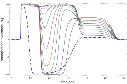
Figure 3: Time dependence (logarithmic scale) of the individual chain-length dependent enantiomeric excesses $ee_{n}\%=\frac{[L_{n}]-[R_{n}]}{[L_{n}]+[R_{n}]}\times 100$, from the start of reactions to chiral symmetry breaking, and then on to the final racemization (family of solid curves). Near $t\simeq 10^{4}$, the sequence of curves from top to bottom corresponds to $n=2$ to $n=12$, respectively. Note damped oscillatory behavior of the excesses corresponding to $n=7,8,9,10,11,12$. The dashed curve shows the chiral excess for the monomers: $ee_{1}\%$. Same initial concentrations and rate constants as in Fig. 1.

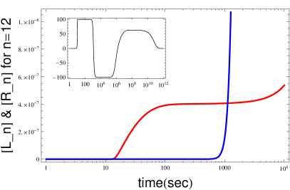
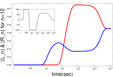
Figure 4: Chiral oscillations. Evolution of the individual concentrations $[L_{12}]$ (the upper curve at the bifurcation) and $[R_{12}]$ for the complete time interval spanning symmetry breaking to final racemization. The inset graph gives the associated percent enantiomeric excess $ee_{12}$ versus time. Left: expanded view of the initial stages of evolution for $1\leq t\lesssim 10^{4}$. Symmetry breaking occurs at $t\sim 10$ with $L_{12}$ dominating the excess. The chiral excess of these longest chains vanishes instantaneously for the first time at around $t=10^{3}$ when the curves intersect, and then turns over such that now $R_{12}$ dominates the chiral excess, see right hand graph (this leads to the sign flip in the excess, see inset). Right: chiral excess vanishes a second time at $t\sim 10^{6}$ when the two curves intersect again (compare to inset). Then from about $10^{6}$ to $10^{11}$ the $L_{12}$ chains again dominate the chiral excess until racemization, when the two curves collapse to a common curve (anti-bifurcation). Same initial concentrations and rate constants as in Fig. 1.

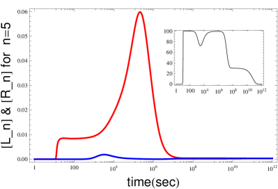
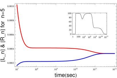
Figure 5: Evolution of the individual concentrations $[L_{5}]$ (the upper curve at the bifurcation) and $[R_{5}]$ for the complete time interval spanning symmetry breaking to final racemization. The inset graph gives the associated percent enantiomeric excess $ee_{5}$ as a function of time. Left: full history of the evolution. Right: close up of the final time scales and racemization (anti-bifurcation).

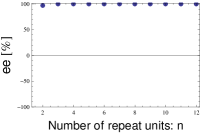
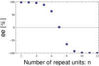
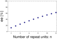
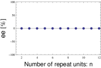
Figure 6: Different time slices or “snap-shots” of Fig 3 showing dependence of the chain-length dependent enantiomeric excesses $ee_{n}\%=\frac{[L_{n}]-[R_{n}]}{[L_{n}]+[R_{n}]}\times 100$ for $n\geq 2$, at different selected time scales. From left to right: total chiral symmetry breaking for all length homopolymer chains at $t=100$, next, second graph shows the sign reversal tendency for the largest chains at $t=10^{4}$, followed by the third graph, the monotone increase of chiral excess as a function if chain length at $t=10^{9}$, and then the fourth graph, the final racemization at $t=10^{13}$. Same initial concentrations and rate constants as in Fig. 1.

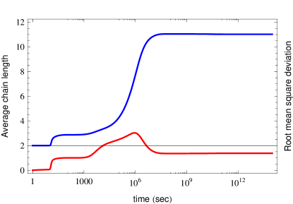
Figure 7: The time evolution (logarithmic scale) of the average or mean homopolymer chain length ${\bar{n}}$ (upper curve) and the corresponding root-mean-square deviation $<\overline{n^{2}}>^{\frac{1}{2}}$ from the mean value (lower curve). The final stable values of the mean and RMS values are ${\bar{n}}=11.02$ and $<\overline{n^{2}}>^{\frac{1}{2}}=1.38$, for $t\gtrsim 10^{7}$. This demonstrates that the final racemic mixture is dominated by the longer length homopolymer chains, and this is the final equilibrium configuration. Same initial concentrations and rate constants as in Fig. 1.

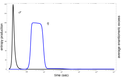
Figure 8: Time evolution (logarithmic time scale) of the average enantiomeric excess $\eta$, averaged over all chains ($2\leq n\leq 12$) Eq. (32), and the associated entropy production $\sigma$, Eq. (18). The entropy production peaks well before ($t\sim 3$) the onset of chiral symmetry breaking ($t\sim 300$) followed by a dramatic decrease to very small values. $\sigma$ strictly approaches zero only at the racemization time scale $t_{racem}\gtrsim 10^{15}$. Initial concentrations: $[L_{1}]_{0}=(1\times 10^{-6}+1\times 10^{-15})M$ and $[R_{1}]_{0}=1\times 10^{-6}M$ ($ee_{0}=5\times 10^{-8}\%$), $[S]_{0}=2M$, all other homo- and heterochiral oligomer initial concentrations are zero; and for the following rates $\epsilon=2\times 10^{-5}$, $\epsilon_{-}=10^{-10}$, $k=2.0$, $k_{-}=10^{-5}$, $f=0.9$, $k_{aa}=k_{bb}=1.0$, $k_{ab}=k_{ba}=20$, $k_{ab}^{-}=k_{ba}^{-}=k_{aa}^{-}=k_{bb}^{-}=10^{-6}$

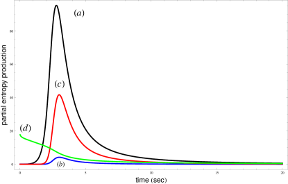
Figure 9: Partial contributions to the total entropy production. From, (a) limited enantioselective monomer catalysis, (b) stepwise polymerization reactions, (c) chain-end termination and heterodimer formation reactions $\times 20$, and (d) direct monomer production $\times 1000$. Same initial concentrations and rate constants as in Fig. 8.

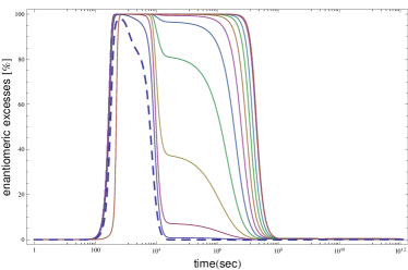
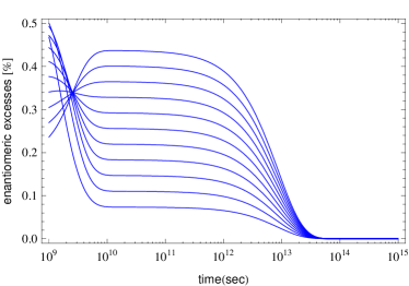
Figure 10: Time dependence (logarithmic scale) of the individual chain-length dependent enantiomeric excesses $ee_{n}\%=\frac{[L_{n}]-[R_{n}]}{[L_{n}]+[R_{n}]}\times 100$, from the start of reactions to chiral symmetry breaking, and then on to the final racemization (family of solid curves). The dashed curve shows the chiral excess for the monomers. Right hand side shows a blow-up of the $ee_{n}$’s for the time scale $t=10^{9}$ to $10^{15}$, exhibiting the sequence of excesses and its final convergence to zero at racemization. Same initial concentrations and rate constants as in Fig. 8.

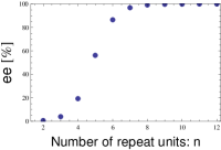
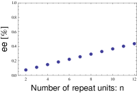
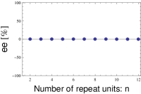
Figure 11: Different time slices or “snap-shots” of Fig 10 showing dependence of the chain-length dependent enantiomeric excesses $ee_{n}\%=\frac{[L_{n}]-[R_{n}]}{[L_{n}]+[R_{n}]}\times 100$ for $n\geq 2$, at different selected time scales. From left to right: total chiral symmetry breaking for all length homopolymer chains at $t=10^{3}$, next, second graph shows the stepwise increase for the largest chains at $t=10^{6}$, followed by the third graph, the monotone increase of chiral excess as a function if chain length at $t=10^{10}$, and then fourth graph, the final racemization at approximately $t=10^{14}$. Same initial concentrations and rate constants as in Fig. 8.

Static “snapshots” of this dynamic behavior nicely complement the evolution of the chain length dependent enantiomeric excesses. In Figure 6 we display the enantiomeric excess versus the number of chiral repeat units at selected time slices. In the leftmost graph, the $ee$’s are all at $100\%$ for all the chains. The next graph, corresponding to $t=10^{4}$, shows the sign reversal tendency as a function of chain length, with the full reversal ($-100\%$) being attained for the largest homochiral chains. The following graph, corresponding to $t=10^{9}$ shows the monotone increase of $ee$ with chain length. Finally, the righthand most graph shows that racemization has set in by $t=10^{13}$. These should be contrasted with Figure 3. It is interesting to point out that both the qualitative behaviors depicted in the second and third snapshot have been reported in two recent and independent polymerization experiments. The tendency of the sign reversal in $ee$ (from positive to negative values) as a function of chain length has been observed in the polymerization of racemic valine (Val-NCA) and leucine (Leu-NCA)in water subject to chiral initiators Lahava . By contrast, the monotonic increase of the percent $ee$ with chain length has been measured in independent chiral amplification experiments using leucine and glycine in water Hitzb starting with a $20\%$ initial enantiomeric excess of the $L_{1}$ monomer. These static snapshots also raise the important question of when to observe the chiral amplification and the enantiomeric excesses. In nonlinear reaction schemes such as this one, the enantiomeric excesses one measures can depend strongly on when the measurement or observation is made, that is, when one decides to terminate the experiment.

Additional information regarding the homo-oligomer composition of the chemical system is provided by the average homochiral chain length $<n>$, see Eq.(33). We plot this in Figure 7 along with the standard deviation about the mean, Eq. (34). The mean chain length starts off at $2$, corresponding to the homodimer and then increases monotonically after the symmetry breaking transition, reaching a constant plateau at $t=10^{7}$ where it remains constant all the way through to racemization and beyond. The final mean value $<n>=11.0$. The corresponding root mean square indicates that the fluctuations in the mean chain length increase as the mean chain length increases but then drops down to a constant value $(\overline{n^{2}})^{1/2}\sim 1.4$ when the average value stabilizes. This indicates that the final racemic composition is dominated by the longer chains: $n_{final}=11.0\pm 1.4$. The racemization time scale depends on how “irreversible” the model is. By way of example, if we increase the rate $k_{-}$ of the reverse catalysis steps in Eq.(1), keeping everything else constant, then the increased recycling of monomers back into achiral precursor $S$ lowers this time scale as follows: $(k_{-},t_{racem})=(10^{-6},5\times 10^{12}s),(10^{-5},5\times 10^{11}s),(10^{-4},5\times 10^{10}s),(10^{-3},1\times 10^{10}s),(10^{-2},5\times 10^{9}s).$ By the same token, if we make $k_{-}$ smaller, we can postpone racemization.

The enantiomeric cross inhibition $k_{ab}=k_{ba}$ is a determining factor in this model. By way of contrast, we consider a second $N=12$ run with a much lower mutual inhibition than employed above, namely $k_{ab}=k_{ba}=20$, and with the following inverse rates all set equal $k_{aa}^{-}=k_{bb}^{-}=k_{ab}^{-}=k_{ba}^{-}=10^{-6}$, but keeping the remainder of the rates as before and with the same initial concentrations and excess. In this situation, the symmetry breaking occurs at a later time and most interestingly, the entropy production now peaks well before the mirror symmetry is broken, see Figure 8. Figure 9 shows that the catalysis still yields the major contribution to this peak, but the second and third most important contributions are now formation of end-chain spoiled oligomers followed by the polymerization, exactly opposite to the previous run employing the much higher mutual inhibition. The peak in $\sigma$ is due principally to monomer catalysis, and not symmetry breaking.

The time dependence of these $n$-dependent $ee$’s is plotted in Figure 10; note the logarithmic time scale. The individual $ee$’s follow a common curve from initialization to chiral symmetry breaking, at about $t\sim 300$, and remain together at nearly $100\%$ until about $t\sim 1000$ at which time the common curve begins to split up into its component parts. Note how the shorter homopolymers tend to racemize before the longer ones, there is a sequential chiral erosion in the individual enantiomeric excesses that is more pronounced the shorter the chain length. This holds as well for the monomer, plotted in the dashed curve (contrast to the monomer behavior in Fig. 3). Then, the percent excess of each length homochiral chain behaves differently, until they again coalesce into a single curve upon final racemization, occurring at around $t\sim 10^{14}$. The final approach to racemization is qualitatively very similar to the case treated above, compare the sequence in the right hand graph of Figure 10; to the sequence of curves in Figure 3 from roughly $t\sim 10^{7}$ to $10^{12}$. A sequence of snap-shots of the $ee_{n}$’s at selected times is displayed in Figure 11.

Finally, we plot the average homochiral chain length $<n>$, see Eq. (33) in Figure 12 along with the standard deviation. The mean chain length starts off at $2$, corresponding to the homodimer and then increases monotonically after the symmetry breaking transition, reaching a constant plateau at about $t=10^{9}$ where it remains constant all the way through to racemization and beyond. The final mean value $<n>=10.9$. Once again, the final racemic composition is dominated by the longest chains.

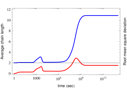
Figure 12: The time evolution (logarithmic scale) of the average or mean homopolymer chain length ${\bar{n}}$ (upper curve) and the corresponding root-mean-square deviation $<\overline{n^{2}}>^{\frac{1}{2}}$ from the mean value (lower curve). The final stable values of the mean and RMS values are ${\bar{n}}=10.9$ and $<\overline{n^{2}}>^{\frac{1}{2}}=1.5$, for $t\gtrsim 10^{10}$. The final racemic mixture is highly dominated by the longer length homopolymer chains, and this is the equilibrium configuration. Same initial concentrations and rate constants as in Fig. 8.

V Conclusions and Discussion

We have demonstrated that a strong chiral amplification can take place in a reversible model of chiral polymerization closed to matter flow and subject to constraints imposed by micro-reversibility. The inherent statistical fluctuations about the idealized racemic composition are modeled by an initial minuscule enantiomeric excess in a system dilute in the monomers. These results are important, because they suggest that spontaneous mirror symmetry breaking in experimental chiral polymerization can take place, and with observable and large chiral excesses without the need to introduce chiral initiators Lahavb or large initial chiral excesses Hitzb . Instead, the needed chiral monomers (i.e., amino acids) can be produced directly from an achiral precursor and amplified via catalysis. Strong mutual inhibition is required to amplify the initial $ee$ to large values, very similar to what we found for the reversible Frank model in closed systems CHMR . The chain-length dependent enantiomeric excesses depend on time in a highly nontrivial way. The essential rate constant is that corresponding to the enantiomeric inhibition. A most intriguing novel feature revealed here for appreciable enantiomeric cross inhibition is the tendency for the chain length dependent enantiomeric excesses to exhibit a damped oscillatory behavior before the onset of final racemization. In these conditions, the observed chiral excess is clearly a time dependent phenomena, though the “period” of the chiral oscillations can be quite long. Oscillatory dynamics in chemical reactions has been observed experimentally, and analyzed theoretically and numerically in simple model systems Scott ; CH ; as far as we are aware, this behavior has not been revealed previously as a valid dynamical solution in polymerization models. The implications for chirality transmission are far reaching: “memory” of the sign of the initial chiral fluctuation is washed-out by the oscillations in the enantiomeric excess, adding another heretofore unexpected element of randomness to the process. While the sign of the initial chiral fluctuation is entirely random, any subsequent chiral oscillations can further “erase” the memory of the sign of this initial enantiomeric excess. These oscillations cease as the system approaches its equilibrium state. Moderate values leads to strong temporary symmetry breaking and larger values can lead to long period damped chiral oscillations before final racemization takes over.

We have also shown that the rate of entropy production per unit volume exhibits a peak value either before or near the vicinity of the chiral symmetry breaking transition. This increase to a peak value is mainly due to the catalytic production of the chiral monomers, followed next by the stepwise polymerization reactions, and then by the chain-end termination reactions and lastly, by the direct monomer production. The rate falls to a vanishingly small but constant nonzero value maintained during the intermediate time scales, then drops to zero once the system has racemized. Previous calculations of the entropy produced in chiral symmetry breaking transitions have been carried out in the Frank model. In KondeKapcha , $\sigma$ was evaluated for a reversible open flow Frank model with a constant inflow of achiral substrate and a constant outflow of the mutual inhibition product. In that situation, the entropy production rises from small initial value and then levels off to a constant plateau after symmetry breaking. As the open flow keeps this system far from equilibrium, it can never racemize, and entropy is produced at a constant rate, in sempiternum. In Mauksch , the rate of entropy production was evaluated for a reversible open flow Frank model including limited enantioselectivity. Mirror symmetry is broken incompletely, and $\sigma$ increases sharply from the start of the reaction, remains at a constant level during the lifetime of the initial racemic state and then decreases to a new stationary value once symmetry breaking sets in. These latter authors also consider the reversible Frank model with constant concentration of substrate but freely varying inhibition product. The entropy production increases, a peak value is reached when symmetry breaking is almost complete, then decreases to very small values. On the other hand, for a reversible Frank model closed to matter flow, and with strong mutual inhibition, the rate of entropy production exhibits a sharp peak at the onset of symmetry breaking, falling to a tiny positive value until the system racemizes, at which time $\sigma$ goes to zero private . This latter behavior is qualitatively similar to what we find in our polymerization model for large inhibition.

For sake of computational simplicity, we have considered a model wherein no generally mixed heteropolymers were formed, only the heterodimer $LR=RL$ and $LR_{n-1}$ and $RL_{n-1}$ for $3\leq n\leq N$. The corresponding number of differential equations grows linearly with the length $N$ as $4N-2$ . A more realistic model should of course include the formation of all the possible heteropolymers of a given length $n$, i.e., those heterochiral chains of length $n$ containing $r\geq 1$ copies of $L_{1}$ and $s\geq 1$ copies of $R_{1}$ such that $r+s=n$. It is possible to build such a system, for example, starting with the copolymerization model of WC2 , where the concentration variables are denoted as $c^{L}_{r,s}(t)|_{r\geq 1,s\geq 0}$ and $c^{R}_{r,s}(t)|_{r\geq 0,s\geq 1}$, the superscript indicating the final monomer in the chain, while the double subscript $r,s$ encodes the number of individual $L$ and $R$’s making up the chain, respectively. The number of differential equations in this case grows quadratically with polymer length $N$ as $N(N+1)$, and is mathematically more involved. Detailed studies employing a reversible copolymerization scheme in closed systems will be presented elsewhere CdTH .

- (1) V. Avetisov and V. Goldanskii, Proc. Natl. Acad. Sci. USA 93 (1996) 11435.
- (2) A. Guijarro and M. Yus, The Origin of Chirality in the Molecules of Life (RSC Publishing, Cambridge, 2009)
- (3) I. Weissbuch, G. Bolbach, H. Zepik, E. Shavit, M. Tang, J. Frey, T.R. Jensen, K. Kajer, L. Leiserowitz and M. Lahav, J. Am. Chem. Soc. 124 (2002) 9093.
- (4) J. Crusats, D. Hochberg, A. Moyano and J.M. Ribó, ChemPhysChem 10 (12) (2009) 2123.
- (5) D.K. Kondepudi, I. Progogine and G. Nelson, Phys. Lett. A 111 (1985) 29; V.A. Avetisov, V.V. Kuz’min and S.A. Aniki, Chem. Phys. 112 (1987) 179.
- (6) P.G.H. Sandars, Origins Life Evol. Bios. 33 (2003) 575.
- (7) A. Brandenburg and T. Multamäki, Int. J. Astrobiology 3 (2004) 209.
- (8) A. Brandenburg, A.C. Andersen, S. Höfner and M. Nilsson, Origins Life Evol. Bios. 35 (2005) 225.
- (9) J.A.D. Wattis and P.V. Coveney, Origins Life Evol. Bios. 35 (2005) 243.
- (10) M. Gleiser and J. Thorarinson, Origins Life Evol. Bios. 36 (2006) 501.
- (11) M. Gleiser, Origins Life Evol. Bios. 37 (2007) 235.
- (12) M. Gleiser and S.I. Walker, Origins Life Evol. Bios. 38 (2008) 293.
- (13) M. Gleiser, J. Thorarinson and S.I. Walker, Origins Life Evol. Bios. 38 (2008) 499.
- (14) Y. Saito and J. Hyuga, J. Phys. Soc. Jpn. 74 (2005) 1629.
- (15) F.C. Frank, Biochim. et Biophys. Acta 11 (1953) 459.
- (16) R. Plasson, H. Bersini and A. Commeyras, Proc. Nat. Acad. Sci. USA 101 (2004) 16733.
- (17) M. Blocher, T. Hitz and P.L. Luisi, Helv. Chim. Acta 84 (2001) 375.
- (18) T. Hitz and P. L. Luisi, Helv. Chim. Acta 86 (2003) 1423.
- (19) J.G. Nery, G. Bolbach, I. Weissbuch and M. Lahav, Angew. Chem. Int. Ed. 42 (2003) 2157.
- (20) T. Hitz and P. L. Luisi, Origins Life Evol. Bios. 34 (2004) 93.
- (21) I. Rubinstein, R. Eliash, G. Bolbach, I. Weissbuch and M. Lahav, Angew. Chem. Int. Ed. 46 (2007) 3710.
- (22) R.A. Illos, F.R. Bisogno, G. Clodic, G. Bolbach, I Weissbuch and M. Lahav, J. Am. Chem. Soc. 130 (2008) 8651.
- (23) I. Rubinstein, G. Clodic, G. Bolbach, I. Weissbuch and M. Lahav, Chem.-Eur. J. 14 (2008) 10999.
- (24) I. Weissbuch, R.A. Illos, G. Bolbach and M. Lahav, Acc. Chem. Res. 42 (8)(2009) 1128.
- (25) K. Mislow, Collect. Czech. Chem. Commun. 68 (2003) 849.
- (26) J.S. Siegel, Chirality 10 (1998) 24.
- (27) U. Stier, J. Chem. Phys. 124 (2006) 024901; ibid. 125 (2006) 024903.
- (28) D. Hochberg, Chem. Phys. Lett. 491 (2010) 237.
- (29) A. Brandenburg, A.C. Andersen and M. Nilsson, Origins Life Evol. Bios. 35 (2005) 507.
- (30) P.M. Chaikin and T.C. Lubensky, Principles of Condensed Matter Physics (Cambridge University Press, Cambridge, 1995), Chap. 3.
- (31) T.F.A. DeGreef, M.M.J. Smulders, M. Wolffs, A.P.H.J Schenning, R.P. Sijbesma and E.W. Meijer, Chem. Rev. (Published Online: September 21, 2009) DOI: 10.1021/cr900181u .
- (32) J. Ross and M. O. Vlad, J. Phys. Chem. A 109 (2005) 10607.
- (33) D. Kondepudi and L. Kapcha, Chirality 20 (2008) 524.
- (34) M. Mauksch and S. B. Tsogoeva, ChemPhysChem 9 (2008) 2359.
- (35) D. Kondepudi and I. Progogine, Modern Thermodynamics: from heat engines to dissipative structures (New York, Wiley, 1998).
- (36) W.H. Mills, Chem. Ind. (London) 10 (1932) 750; V.I. Goldanski and V.V. Kuzmin, Z. Phys. Chem. (Leipzig) 269 (1988) 269.
- (37) J.M. Ribó, private communication.
- (38) S.K. Scott, Oscillations, Waves, and Chaos in Chemical Kinetics (Oxford University Press, Oxford, 1994).
- (39) M.C. Cross and P.C. Hohenberg, Rev. Mod. Phys. 65 (1993) 851.
- (40) J.A. Wattis and P.V. Coveney, J. Phys. Chem. B 111 (2007) 9546.
- (41) C. Blanco and D. Hochberg, work in progress.