PLASMA HEATING DURING A CORONAL MASS EJECTION OBSERVED BY SOHO

Abstract

We perform a time-dependent ionization analysis to constrain plasma heating requirements during a fast partial halo coronal mass ejection (CME) observed on 2000 June 28 by the Ultraviolet Coronagraph Spectrometer (UVCS) aboard the Solar and Heliospheric Observatory (SOHO). We use two methods to derive densities from the UVCS measurements, including a density sensitive O V line ratio at 1213.85 and 1218.35 Å, and radiative pumping of the O VI $\lambda\lambda$1032,1038 doublet by chromospheric emission lines. The most strongly constrained feature shows cumulative plasma heating comparable to or greater than the kinetic energy, while features observed earlier during the event show cumulative plasma heating of order or less than the kinetic energy. SOHO Michelson Doppler Imager (MDI) observations are used to estimate the active region magnetic energy. We consider candidate plasma heating mechanisms and provide constraints when possible. Because this CME was associated with a relatively weak flare, the contribution by flare energy (e.g., through thermal conduction or energetic particles) is probably small; however, the flare may have been partially behind the limb. Wave heating by photospheric motions requires heating rates significantly larger than those previously inferred for coronal holes, but the eruption itself could drive waves which heat the plasma. Heating by small-scale reconnection in the flux rope or by the CME current sheet is not significantly constrained. UVCS line widths suggest that turbulence must be replenished continually and dissipated on time scales shorter than the propagation time in order to be an intermediate step in CME heating.

1. INTRODUCTION

The understanding of astrophysical phenomena generally begins with the energy budget. The energy budgets of coronal mass ejections (CMEs) include contributions from magnetic energy, bulk kinetic energy, ionization energy, gravitational potential energy, thermal energy, and energetic particles (e.g., Emslie et al., 2005). Energy can be lost to the system through radiation and thermal conduction. White light observations from instruments such as the Large Angle Spectroscopic Coronagraph (LASCO; Brueckner et al., 1995) on board the Solar and Heliospheric Observatory (SOHO) allow a straightforward determination of the contributions by kinetic and gravitational energy (e.g., Vourlidas et al., 2000, 2010; Subramanian & Vourlidas, 2007). The magnetic energy is thought to be the largest component of the CME energy budget but is difficult to constrain via remote sensing because of the lack of good magnetic field diagnostics, especially for transient events such as CMEs. However, the total and free magnetic energy of precursor active regions can be estimated using vector magnetograms (e.g., Metcalf et al., 2005), line-of-sight magnetograms from the Michelson Doppler Imager (MDI) on SOHO, and empirical relationships between X-ray luminosity and magnetic flux (Fisher et al., 1998). The magnetic field structure of interplanetary coronal mass ejections (ICMEs) can be investigated using in situ measurements (see Zurbuchen & Richardson, 2006, and references therein) by spacecraft such as the Advanced Composition Explorer (ACE).

Several different lines of evidence now suggest that the thermal energy input into CMEs is comparable to the kinetic energy of the ejected plasma. First, observations between 1.5 and 3.5 solar radii by the Ultraviolet Coronagraph Spectrometer (UVCS; Kohl et al., 1995, 2006) on board SOHO have been analyzed using a time-dependent ionization code for four prior events (Akmal et al., 2001; Ciaravella et al., 2001; Lee et al., 2009; Landi et al., 2010). The thermal energy input was constrained to be comparable to or greater than the kinetic energy for several features during each of these events. This method is used in this paper and further described in Section 5. Second, in situ measurements of ICMEs typically show high ion charge states (e.g., Lepri et al., 2001; Lynch et al., 2003; Lepri & Zurbuchen, 2004), although low charge state plasma is sometimes observed (e.g., Lepri & Zurbuchen, 2010). Detailed models of ICMEs by Rakowski et al. (2007) showed that continual heating was required out to several solar radii to be consistent with the observed charge states of both iron and oxygen at 1 AU, with total heating requirements again found to be comparable to the CME kinetic energy (see also Gruesbeck et al., 2011). Third, Filippov & Koutchmy (2002) presented observations of a rising prominence by the Transition Region and Coronal Explorer (TRACE). During the eruption, the feature seen at 171 Å suddenly changed from absorption to emission by the prominence, indicating significant and rapid heating. Fourth, Liu et al. (2006) investigated in situ measurements between $0.3$ and $20$ AU and found that dissipation of turbulence can explain the observed heating rates. The turbulence generation mechanism is not understood in the inner heliosphere but heating by pickup ions contribute to ICME heating in the outer heliosphere.

Several analytical models explore the energetics of expanding flux ropes. Kumar & Rust (1996, hereafter, KR) assume global conservation of mass, magnetic flux, and helicity for a self-similarly expanding force-free flux rope. The magnetic energy is found to decrease monotonically during the process of expansion. Some of the lost magnetic energy goes into overcoming solar gravity and increasing the bulk kinetic energy, but a large fraction is presumed to go into heating the plasma within the expanding flux rope. Wang et al. (2009) develop a different model of a self-similarly expanding flux rope which relaxes several assumptions made by KR and implicitly includes some effects associated with the solar wind. Their inference of a CME polytropic index of $\frac{4}{3}$ for one event indicates continued heating during flux rope expansion. Lyutikov & Gourgouliatos (2010) model CME flux ropes as expanding force-free spheromaks. By allowing for finite dissipation during expansion and assuming a large anomalous resistivity (e.g., due to wave-particle interactions), Rakowski et al. (2011) show that this model can reproduce charge states observed within the flux rope, but not the higher charge states such as Fe¹⁶⁺ in the plasma trailing the flux rope.

However, none of these models specify the physical mechanisms responsible for plasma heating. The most likely candidate is dissipation of magnetic energy. There are several candidate mechanisms, which are discussed in detail in Section 8. These include upflow from the CME current sheet, kinking of the CME flux rope, small-scale reconnection or tearing behavior within the CME ejecta, waves driven by either photospheric motions or by the eruption itself, thermal conduction, and deposition of energy by energetic particles. Additionally, Filippov & Koutchmy (2002) argue that colliding flows along flux tubes can heat prominence plasma to coronal temperatures in upward concave regions of flux tubes.

In this paper we use a time-dependent ionization analysis to constrain the thermal energy content and plasma heating of a fast CME observed by SOHO on 2000 June 28. This technique has previously been used to investigate heating during four slow CMEs observed by SOHO/UVCS (see Table 1). Akmal et al. (2001) analyzed a CME on 1999 April 23 and found that the cumulative heating energy was comparable to the kinetic and gravitational potential energy of this event. There was a core of cool plasma radiating in C iii which was surrounded by hotter material radiating in O vi. Ciaravella et al. (2001) analyzed a CME on 1997 December 2 and found that gradual heat release mechanisms are probably more appropriate than mechanisms where heating is concentrated during the early evolution of a CME. Lee et al. (2009) investigated a CME observed on 2001 December 13 and constrained the cumulative heating energy for the bright knots observed in O vi to be greater than the kinetic energy. Landi et al. (2010) analyzed the ‘Cartwheel CME’ observed by SOHO, Hinode, and STEREO on 2008 April 9 and again found that the cumulative heating energy was constrained to be greater than the kinetic energy. Both Lee et al. (2009) and Landi et al. (2010) show that thermal conduction is probably too slow to sufficiently heat the CME plasma during the early evolution of the flux rope. Using different methods, Bemporad et al. (2007) investigated a slow flareless CME observed by UVCS and the Large Angle and Spectrometric Coronagraph Experiment (LASCO) on 2000 January 31 and found that the core and leading edge of the CME were hotter than the ambient corona.

Table 1Census of CME energy budget papers using the technique of Akmal et al. (2001)

Event	$V_{\mathrm{POS}}$ (km/s)	Mass (g)	Reference
1997 Dec 12	$211$	$2.9\times 10^{14}$	Ciaravella et al. (2001)
1999 Apr 23	$523$	$2.7\times 10^{15}$	Akmal et al. (2001)
2000 Jun 28	$1198$	$7.3\times 10^{15}$	Murphy et al. (2011)
2001 Dec 13	$864$	—	Lee et al. (2009)
2008 Apr 9	$650$	$1.4\times 10^{15}$	Landi et al. (2010)

The 2000 June 28 CME analyzed in this paper has been previously investigated in multiple separate works. Raymond & Ciaravella (2004) used radiative pumping of the O vi $\lambda\lambda 1032,1038$ doublet observed by UVCS to find number densities ranging from $\sim$$1.28\times 10^{6}$–$4\times 10^{7}$ cm^-3. This method is described further in Section 5 and is used in this work to find densities for several features along the UVCS slit. Ciaravella et al. (2005) used UVCS and LASCO observations to identify the leading edge of this CME as a fast mode shock front. Maričić et al. (2006) studied the kinematics of the prominence and leading edge of this CME with LASCO and the Mark IV (MK4) coronagraph at the Mauna Loa Solar Observatory (MLSO). This CME has also been identified as a solar energetic particle (SEP) event (Ho et al., 2003; Wang et al., 2006).

The organization of this paper is as follows. In Section 2, we discuss the methods we use to find densities using UVCS spectra. Observations of the 2000 June 28 CME are described in Section 3. Section 4 identifies UVCS features that have good density diagnostics. The method for our time-dependendent ionization analysis of this event is described in Section 5. A discussion of the results of this analysis is presented in Section 6. The magnetic energy of the precursor active region is estimated in Section 7. Constraints on candidate heating mechanisms are discussed in Section 8. Section 9 contains a summary and conclusions.

2. DENSITY DIAGNOSTICS

A key component of the time-dependent ionization analysis performed in this paper is the electron number density at the location in the corona observed by UVCS. Knowledge of the UVCS density allows us to exclude a significant portion of parameter space when using the method described in Section 5. In this section we discuss our two primary density diagnostics: a classical density sensitive O v line ratio (Akmal et al., 2001) and radiative pumping of the O vi doublet by chromospheric lines (Raymond & Ciaravella, 2004).

2.1. The density-sensitive $\lambda\lambda 1213,1218$ O v line ratio

The ratio of the [O v] forbidden line at 1213.85 Å to the O v] intercombination line at 1218.35 Å is a useful diagnostic for coronal densities of $\sim$$10^{6}$ cm^-3 (Akmal et al., 2001) and is based on well-understood atomic physics. At high densities the forbidden line is weak because of collisional deexcitation. These lines occur at equilibrium temperatures of $\sim$$2\times 10^{5}$ K. We use the CHIANTI database (Dere et al., 1997, 2009), which includes proton collisions. The intensity ratio of these two lines, $I_{1213}/I_{1218}$, is shown as a function of electron number density in Figure 1.

Figure 1.— The ratio of the [O v] line at 1213.85 Å to the O v] line at 1218.67 Å as a function of electron density at $2.24\times 10^{5}$ K.

The [O v] and O v] lines straddle Ly$\alpha$ at 1215.67 Å. Bright Ly$\alpha$ emission can obscure weak [O v] emission to make it difficult to get an accurate line strength for O v]. Moreover, because of the construction of UVCS (described in Section 3.4), the secondary channel [O v] line sometimes appears at the same location on the detector as the primary channel N iii $\lambda 991.58$ Å line. Therefore, this density diagnostic is most useful at certain instrument-dependent line-of-sight velocities and when Ly$\alpha$ emission is relatively weak, but has the advantage that it is weakly dependent on temperature.

2.2. Radiative pumping of O VI

The second density diagnostic is the intensity ratio of O vi $\lambda 1031.91$ to O vi $\lambda 1037.61$. When collisional excitation dominates, the ratio will be 2:1. Departures from this ratio are due to radiative pumping of O vi $\lambda 1037$ by C ii $\lambda\lambda 1036.3$, $1037.0$ near velocities of 172 and 371 km s^-1, O vi $\lambda 1037$ by O vi $\lambda 1032$ near velocities of 1650 km s^-1, or O vi $\lambda 1032$ by Ly$\beta$ near velocities of 1810 km s^-1 (Noci et al., 1987; Raymond & Ciaravella, 2004).

The electron number densities are given as follows. For pumping of O vi $\lambda 1037.61$ by C ii $\lambda 1036.3$ near velocities of 371 km s^-1 (see also Noci et al., 1987), the ratio is less than 2:1 and the number density is given by

$$n_{e}=\frac{\sigma_{1037}I_{\mathrm{disk}}(\mbox{{\rm C}~{}{\sc ii}})W}{q_{1037}}\frac{2-R}{2R}.$$ (1)

For pumping of O vi $\lambda 1037.61$ by O vi $\lambda 1031.91$ near velocities of 1650 km s^-1, the ratio is less than 2:1 and the number density is given by

$$n_{e}=\frac{\sigma_{1037}I_{\mathrm{disk}}(1032)W}{q_{1037}}\frac{2-R}{2R}.$$ (2)

For pumping of O vi $\lambda 1031.91$ by Ly$\beta$ near velocities of 1810 km s^-1, the ratio is greater than 2:1 and the number density is given by

$$n_{e}=\frac{\sigma_{1032}I_{\mathrm{disk}}(\mbox{{\rm Ly}{$\beta$}})W}{q_{1032}}\frac{2}{R-2}.$$ (3)

In the above relations, $\sigma_{1032}$ and $\sigma_{1037}$ are the effective scatting cross sections, $I_{\mathrm{disk}}$ is the solar disk intensity of each of the lines, $W\equiv 2\pi\left(1-\sqrt{1-r^{-2}}\right)$ is the dilution factor for a distance $r$ from Sun center, $q_{\mathrm{1032}}$ and $q_{\mathrm{1037}}$ are the collisional excitation rate coefficients, and $R\equiv I_{1032}/I_{1038}$ is the intensity ratio of the two O vi lines.

This density diagnostic requires more assumptions than the O v density sensitive line ratio. The caveats of this method are discussed by Raymond & Ciaravella (2004) and include that the solar disk intensity of each of the illuminating lines may be enhanced early during flares (Raymond et al., 2007; Johnson et al., 2011), multiple components to the plasma can exist at different speeds along the line of sight, and the collisional excitation rate depends relatively strongly on the temperature of the plasma. In addition, weak C ii $\lambda\lambda 1036.3$, $1037.0$ lines complicate the process of finding the O vi line ratio from observational data. We mitigate the effects of these C ii lines by fitting Gaussian line profiles to Ly$\beta$ and the O vi doublet and enforcing that both lines in the O vi doublet have the same width. In Section 4 we compare the densities derived through both the O v and O vi diagnostics for one particular feature (blob E) and find that the results are consistent to within expected systematic uncertainties.

3. DATA SET

Observations of the CME on 2000 June 28 are available from the EIT, LASCO, and UVCS instruments on board SOHO, and the MK4 coronagraph at MLSO. The C class flare associated with this CME was detected by GOES. Pre-CME and post-CME observations of this event were made by Yohkoh/SXT and SOHO/MDI. The observations for this event have been previously described by Ciaravella et al. (2005) and Maričić et al. (2006), which we summarize below.

3.1. SOHO/EIT observations

SOHO/EIT images in the 195 Å band were taken with a $\sim$$12$ minute cadence during most of this event. Between 19:00:14 and 19:19:44 UT, EIT images at 171 Å, 284 Å, 195 Å, and 304 Å were taken in order with a six minute cadence. Several of these observations are shown in Figure 2 from 18:00 UT until 19:36 UT (see also Ciaravella et al., 2005, Figure 1). The series of 195 Å observations shows a dark arcade near the northwest limb starting to rise around 18:00:10 UT. That it is dark at 195 Å indicates the absence of plasma at $\sim$1 MK in the rising structure. Between 18:36:10 and 18:48:12 UT, this feature rises rapidly and is not apparent in the next 195 Å observation at 19:13:48 UT. The 304 Å image at 19:19:44 UT shows bright strands indicative of He ii emission, suggesting that the rising filament was relatively cool. The 195 Å images at 19:26:04 and 19:36:24 UT show a thin strand of hot plasma that outlines the He ii arch in the 304 Å image at 19:19:44 UT, indicating the presence of some plasma around 1 MK associated with the strand. These strands are probably associated with the feature identified in Section 4 as blob F.

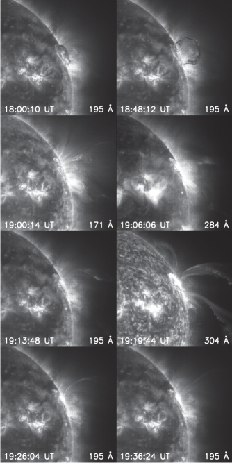
Figure 2.— SOHO/EIT observations of the 2000 June 28 CME, rescaled to emphasize faint structure.

3.2. MLSO/MK4 observations

MLSO/MK4 measures the polarization brightness (pB) of the corona between $\sim$$1.1$ and $\sim$$2.8$ solar radii using radial scans with a cadence of about three minutes. MK4 observations were performed on the day of the event between 16:56 and 20:00 UT. A time sequence of the eruption is presented in Figure 3.

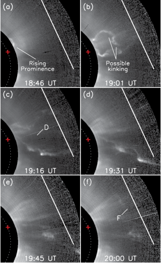
Figure 3.— MLSO/MK4 polarization brightness observations of the 2000 June 28 CME, rescaled to emphasize faint structure. Estimated positions of the features observed by UVCS and discussed in Section 4 are labeled. The position of the precursor active region is denoted by the red plus sign.

The first clear sign of the CME was at 18:46 UT when a rising bright arch entered the field of view (see Figure 3a). We identify this arch as the erupting filament observed by EIT, most notably at 18:48 UT (see Figure 2). Consequently, this filament is observed simultaneously by EIT and MK4. The kinematics of this rising prominence were presented by Maričić et al. (2006). The prominence was accelerated most strongly between $\sim$18:40 and $\sim$19:00 UT at up to $\sim$$0.5$ km s^-2. The upper parts of this arch begin to fade around 19:01 UT (Figure 3b) and are not apparent by 19:16 UT (Figure 3c).

After about 18:49 UT, the rising loop developed a twisted or helical structure. This behavior is consistent with the onset and nonlinear growth of a long wavelength kink instability, and is apparent in the observation at 19:01 UT (Figure 3b). A bright stream of ejecta directed towards the southwest is observed to miss the UVCS slit entirely (Figure 3c–d). A faint feature rising at $V_{\mathrm{POS}}\approx$250 km s^-1 is observed around 20:00 UT when the set of observations ends, which we identify in Section 4 as Blob F.

3.3. SOHO/LASCO white light observations

SOHO/LASCO performs white light observations of the solar corona between 2.5 and 30 solar radii. Observations of the 2000 June 28 CME were performed by both the C2 and C3 cameras for the duration of the event. The first C2 observation at 19:31:55 UT of the eruption showed a large plume of plasma off of the west limb (see Figure 4). The flux rope observed by EIT and MK4 had by this time broken up into several different outwardly propagating blobs. In subsequent C2 observations at 19:54:41 and 20:06:05 UT, each of the clouds propagated approximately radially outward from the location of the flare site and rising prominence with some expansion. The C2 image at 20:30:05 UT shows the loop identified as Blob F in Section 4 slowly rising above the center of the UVCS slit. This feature was probably ejected late during the eruption.

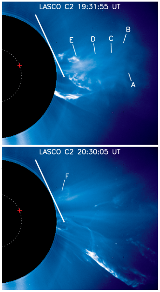
Figure 4.— LASCO C2 white light observations of this event, rescaled to emphasize faint structure. The approximate locations of the features observed by UVCS and analyzed using a time-dependent ionization code are labeled. The plane of sky velocities for these features were estimated using either O vi pumping information or complementary MLSO/MK4 observations. The precursor active region is denoted by the red plus sign.

Observations by both the C2 and C3 cameras show a bright stream of plasma propagating approximately radially outward from the region of the flare site. Unfortunately, this feature passed just south of the UVCS slit. The feature exhibited significant expansion during propagation. The apparent velocity of this feature was $\sim$$300$ km s^-1 at the low altitude end and $\sim$$600$ km s^-1 at the high altitude end while in the C2 field of view.

The LASCO CME Catalog estimates a mass of $\sim$$7.3\times 10^{15}$ g and a kinetic energy of $\sim$$5.3\times 10^{31}$ ergs. This corresponds to a kinetic energy per unit mass of $\sim$$73\times 10^{14}$ ergs g^-1. However, the mass of this event is uncertain because this was a partial halo CME; furthermore, the kinetic energy is uncertain because it assumes that the entire plasma is propagating at the same velocity, and only considers the plane-of-sky velocity.

3.4. SOHO/UVCS observations

SOHO/UVCS (Kohl et al., 1995, 2006) is a long slit spectrograph designed to study the solar corona at 1.5–10 solar radii. The use of both internal and external occulters keeps stray light at low enough levels to observe the faint corona. The UVCS O vi channel contains two spectrometer light paths optimized for the O vi $\lambda\lambda 1032,1038$ doublet (primary) and Ly$\alpha$ (redundant). Throughout the course of this event, the UVCS entrance slit was positioned at $\rho=2.32R_{\odot}$ with a position angle of $295^{\circ}$ over the precursor active region near the northwest limb. The exposure time was two minutes, thus allowing high time resolution observations of the ejecta. The slit width was $49$ $\mu$m. The observations are available in three wavelength ranges (denoted panels): 976–979 Å, which contains the C iii $\lambda$977 line; 1024–1045 Å, which contains the O vi $\lambda$1032,1038 doublet and H i Ly$\beta$; and 1210–1220 Å, which contains H i Ly$\alpha$ and the forbidden and intercombination lines of O v at 1213 Å and 1218 Å, respectively. Because the positions on the detector overlap between the different channels, the primary channel N iii $\lambda$989,991 doublet appears in the Ly$\alpha$ panel at different wavelengths depending on the redshift. Because of telemetry limitations, the UVCS observations were binned in three pixels in the spatial direction for a resolution of $21^{\prime\prime}$ per bin, and two pixels in the spectral direction for a resolution of 0.198 Å (57 km s^-1) for the C iii and O vi panels and 0.183 Å (45 km s^-1) in the Ly$\alpha$ channel.

The UVCS observations of this event are summarized in detail by Ciaravella et al. (2005). Starting in the exposure at 18:59, UVCS detected faint, diffuse, and broad blueshifted O vi emission at position angles of 273–295^∘, indicating passage of the CME front. Knots bright in O vi and Ly$\alpha$ first appear at 19:06 UT at a position angle of 273^∘. At 19:12 UT, a blueshifted bright knot in O vi and Ly$\alpha$ appears at 277^∘ (see Figure 5; this is associated with blob A). This indicates the passage of cooler prominence plasma. By 19:14 UT, these knots fill the spatial direction along the slit between $\mathrm{P.A.}=272^{\circ}$ and $290^{\circ}$. Shortly after, two knots persist in the UVCS observations but the southern knot fades by about 19:30 UT. For many of the features early in the event, Ly$\beta$, [O v], and C iii were off-panel because of the very large blueshifts. The northern knot persists for a while but drifts southward. Between 20:09 and 20:13 UT, a new diagonal or shear flow feature appears between $\mathrm{P.A.}=288^{\circ}$–$297^{\circ}$ that has apparent O v], O vi, and C iii emission but little Ly$\alpha$ or Ly$\beta$. A few plasma streams persist afterward as the corona settles back into an undisturbed state.

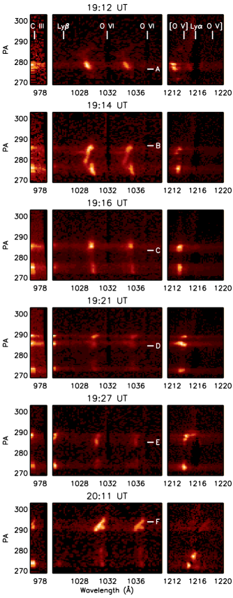
Figure 5.— UVCS observations of each of the features identified in Section 4, rescaled to emphasize faint structure. The pre-CME average background has been subtracted. From left to right are the C iii panel, the O vi panel, and the Ly$\alpha$ panel. The rest wavelengths of the features are shown in the top row.

3.5. GOES X-ray observations

A C class flare was observed by GOES starting at 18:48 UT with the decay continuing until about two hours after the event. Using the GOES $1$–$8$ Å light curve and subtracting the background flux, we estimate that the amount of flare energy emitted in this band is $E_{X}\sim 3\times 10^{28}$ ergs over the entire event. Assuming $L_{\mathrm{tot}}/L_{\mathrm{X}}=100$ (e.g., Emslie et al., 2005), this corresponds to an upper limit of flare energy averaged over the CME of $\lesssim$$4\times 10^{14}$ ergs g^-1. This quantity is about an order of magnitude less than the kinetic energy per unit mass derived from the LASCO CME catalog.

3.6. Yohkoh/SXT observations

Yohkoh/SXT (Tsuneta et al., 1991) performed pre-flare observations including the precursor active region (AR 9046) from 12:00 UT until 13:54 UT and from 15:26 UT until 16:35 UT. Post-flare observations were taken from 19:26–19:46 UT. All three data sets used the thin aluminum filter. There were no other bright X-ray sources in the SXT field of view during this time. No observations were taken during the peak intensity phase of the GOES flare. The observation at 16:50 UT shows that much of the soft X-ray emission from the precursor active region was behind the limb. The observations at 19:26 and 19:50 UT, however, show some new bright X-ray emission in front of the limb. Because of the gap in SXT observations, we cannot rule out the possibility that the flare site was behind the limb and thus partially occulted. However, as shown most recently by Aarnio et al. (2010), it is possible to have powerful and massive CMEs associated with relatively weak flares (see also Reeves & Forbes, 2005).

3.7. SOHO/MDI observations

SOHO/MDI (Scherrer et al., 1995) takes high spectral resolution images of the Ni i $\lambda$6768 absorption line to characterize velocity oscillations and Zeeman splitting in the photosphere. Full disk magnetograms were taken every 96 minutes. A subsection of the magnetogram was taken to match the field of view and orientation of the SXT observations. We use level 1.8 line-of-sight magnetograms to measure the magnetic field and then estimate the magnetic energy of the active region prior to the event. We have included in our analysis magnetograms for 2000 June 25–28. On 2000 June 28, the flaring active region was on the limb. Due to the lack of resolution near the limb and in order to better characterize the magnetic energy associated with the active region, we include in our analysis magnetograms from 2000 June 25 when AR 9046 was on disk.

4. FEATURE IDENTIFICATION AND CHARACTERISTICS

In this section we identify six features observed by both UVCS and LASCO with good density diagnostics. The positions and UVCS observation times of these features are shown in Table 2, along with the lines which were detected, undetected, or off of the UVCS panels. Additional properties of these features are shown in Table 3.

Table 2Features observed by UVCS

Blob	Time	P.A.	$\rho/R_{\odot}$	Observed lines	Upper limits	Off-panel
A	19:12	276∘	2.45	O vi, Ly$\alpha$, N iii	C ii, O v]	[O v], C iii, Ly$\beta$
B	19:14	287∘	2.35	O vi, Ly$\alpha$, C ii, N iii $\lambda$992	O v], N iii $\lambda$990	[O v], C iii, Ly$\beta$
C	19:16	283∘	2.37	O vi, Ly$\alpha$, C ii	O v], N iii	[O v], C iii, Ly$\beta$
D	19:21	284∘	2.36	O vi, Ly$\alpha$	O v], C ii, N iii	[O v], C iii, Ly$\beta$
E	19:27	285∘	2.35	O vi, O v], [O v], Ly$\alpha$, C ii $\lambda$1037.0	C ii $\lambda$1036.3, N iii	C iii, Ly$\beta$
F	20:11	294∘	2.32	O vi, O v], [O v], C iii, N iii $\lambda$992	Ly$\alpha$, Ly$\beta$, C ii, N iii $\lambda$990	—

Table 3Blobs Observed by UVCS

	O vi					O v		Ly$\alpha$	LASCO
Blob No.	$I_{1032}/I_{1037}$	$T_{\mathrm{max}}$	$V_{LOS}$	$V_{POS}$	$\log n_{e}$	$I_{1213}/I_{1218}$	$\log n_{e}$	$T_{\mathrm{max}}$	$N_{e,\mathrm{max}}$
A	1.72	30	-759	1465	7.0	…	…	2.0	23
B	2.21	24	-730	1656	7.5	…	…	2.5	19
C	2.60	39	-735	1654	7.0	…	…	2.5	22
D	1.67	29	-616	1531	6.9	…	…	4.3	20
E	3.73	8.7	-470	1748	6.6	$0.16$–$0.5$	$6.2$–$6.8$	0.9	53
F	2.14	20	-331	250	…	$0.16$	$6.8$	…	7.5

Note. — Key quantities derived for each of the features presented in Section 4. $I_{1032}/I_{1037}$ and $I_{1213}/I_{1218}$ are the line ratios used for the O vi and O v density diagnostics, respectively, described in Section 2. The line-of-sight and plane-of-sky velocities, $V_{\mathrm{LOS}}$ and $V_{\mathrm{POS}}$, are given in km s^-1. The plane-of-sky velocities were derived using O vi pumping information for blobs A–E and MK4 observations for blob F. The number densities derived from these diagnostics are in units of cm^-3. $T_{\mathrm{max}}$ is the maximum temperature in MK for each species allowed from UVCS line widths. $N_{e,\mathrm{max}}$ is the maximum allowed column density from LASCO observations in units of $10^{16}$ cm^-2.

Blobs A and B correspond to the first clear detections of CME prominence plasma at their respective positions along the UVCS slit. There is strong O vi and Ly$\alpha$ emission, with probable detections of N iii. The large blueshifts of $759$ and $730$ km s^-1, respectively, indicate that Ly$\beta$, C iii, and [O v] are off of the UVCS panel. The O v] line is obscured by bright Ly$\alpha$, but upper limits of O v] are obtained. The densities are found through radiative pumping of the O vi doublet to be $\sim$$1\times 10^{7}$ cm^-3 for blob A and $\sim$$3\times 10^{7}$ cm^-3 for blob B.

Blobs C and D are located spatially between the locations of blobs A and B along the UVCS slit but are observed by UVCS a few minutes later. The Ly$\beta$, [O v], and C iii lines are once again off-panel but upper limits of O v] are still possible despite bright Ly$\alpha$. Again, radiative pumping of O vi is used to estimate number densities of $\sim$$1\times 10^{7}$ cm^-3 for blob C and $\sim$$8\times 10^{6}$ cm^-3 for blob D.

Blob E is the first feature observed by UVCS with clear detections of both [O v] and O v], allowing the density to be found using the intensity ratio between these two lines. The ratio of the O vi lines is $I_{1032}/I_{1038}=3.73$, which is substantially different from the collisional ratio of 2:1 and is indicative of significant radiative pumping of the O vi $\lambda 1032$ line. Pumping of this line by chromospheric Ly$\beta$ indicates a total velocity of about 1810 km s^-1, which is large compared to $V_{\mathrm{LOS}}\approx-470$ km s^-1. The density inferred from O vi radiative pumping is $n_{e}\sim 4\times 10^{6}$ cm^-3. This is within the range of densities derived from the O v line ratio of $1.5$–$6\times 10^{6}$ cm^-3. This interpretation implies that $V_{\mathrm{POS}}\gg V_{\mathrm{LOS}}$, that this material is propagating close to the plane of sky, and that this plasma was ejected perhaps $\sim$10–20 minutes after the initial eruption.

A less likely possibility to explain the O vi ratio observed in Blob E is that the O vi $\lambda 1032$ line was being radiatively pumped by chromospheric O i $\lambda\lambda 1027,1028$ emission at velocities near 1100 and 1300 km s^-1. According to the SUMER spectral atlas of the solar disk presented by Curdt et al. (2001), these two lines are about an order of magnitude fainter than chromospheric Ly$\beta$. Consequently, this interpretation would imply that the number density is an order of magnitude smaller than inferred using the assumption of radiative pumping of O vi $\lambda$1032 by Ly$\beta$. Because the number density derived using the assumption of radiative pumping by Ly$\beta$ is consistent with the number density derived from the O v line ratio, we conclude that radiative pumping by Ly$\beta$ is much more likely.

Blob F is observed by UVCS much later in the event (20:11 UT). We identify Blob F as the rising filament structure observed earlier by EIT and MK4. This blob appears as a diagonal shear flow feature in UVCS in O v and O vi emission. There is C iii emission with a different morphology, suggesting that the cool gas is included at least partially in a different component along the line of sight (see also Akmal et al., 2001; Lee et al., 2009). Ly$\alpha$ and Ly$\beta$ emission are both largely absent. Consequently, both [O v] and O v] are easily identified. The O v line ratio is used to derive a density of $n_{e}\sim 6\times 10^{6}$ cm^-3.

Column densities for each of these features are found using LASCO C2 observations rather than MK4 data because of the better signal to noise near the UVCS slit position. The mass per pixel for each C2 observation is found using the C2_MASSIMG function provided by A. Vourlidas in SolarSoft IDL. Because of the relatively low cadence of C2 observations, the C2 position for each feature is estimated by assuming that the plasma from each feature continues propagating on the direct path between the flare site and the position on the UVCS slit where it was observed. The plane-of-sky velocity is assumed to be constant and is found using blueshifts and O vi pumping information (for blobs A–E) or MK4 observations for (blob F). C2_MASSIMG assumes that the ejecta are propagating in the plane of the sky so we use the ratio of $V_{\mathrm{POS}}$ and $V_{\mathrm{LOS}}$ to correct for the dilution factor and Thomson scattering angle. We assume that the column density in C2 observations goes down as $l^{-2}$, where $l$ is the apparent distance from the flare site. Because there will be some departure from a constant velocity, we choose the largest column density within an apparent radius of 0.1 to 0.3$R_{\odot}$, depending on the estimated distance travelled between the UVCS and C2 observations. The results are shown in Table 3 and will be used to constrain the ionization fraction of O vi in the following sections.

5. METHOD

To estimate plasma heating rates for the features described in Section 4, we use a one-dimensional time-dependent ionization code to track the ionization states of the plasma between the flare site and when the features were observed by UVCS. The numerical method has been described in detail by Akmal et al. (2001) and Lee et al. (2009), and we discuss key features here.

Because we do not know the initial state of the plasma before the eruption, we run a grid of models with different initial densities, initial temperatures, heating rates, and heating parameterizations. The initial densities are assumed to be in the range $\log{\left(n/\mbox{cm}^{-3}\right)}\in[8.6,11.6]$. The initial temperatures are assumed to be in the range $\log\left(T/\rm{K}\right)\in[4.6,6.6]$. Consequently, the ejecta are allowed to be cool prominence plasma at relatively high densities or hot plasma from the ambient corona at lower densities. The final densities are presented in Table 3 and were found using one or both of the diagnostics discussed in Section 2. The determination of final density provides a significant constraint on parameter space. The velocity curve is scaled from the prominence velocity curve for this event shown in Figure 2b of Maričić et al. (2006). This velocity curve includes an acceleration phase at low velocity. The ejecta are assumed to be expanding homologously.

We use four different heating parameterizations which we chose for simplicity and consistency with previous work. These simple parameterizations allow us to explore parameter space and the spatial dependence of heating. The first parameterization is the wave heating model for the fast solar wind presented by Allen et al. (1998), denoted by $Q_{\mathrm{AHH}}\propto\exp\left(-d/0.7R_{\odot}\right)$, where $d$ is height above the limb. This is physically motivated by wave heating models of the solar corona. While there may be departures from an exponential if, for example, the Alfvén speed changes with altitude, this form is a reasonable approximation that allows for a gradual decrease of heating with height that does not depend on density or lead to excessive heating far from the flare site. The second parameterization is heating proportional to number density, $Q\propto n$, which also gives strong heating at low heights with a gradual decrease at higher altitudes. The third parameterization is heating proportional to the number density squared, $Q\propto n^{2}$, which concentrates heating at low heights where the density is large and has the same density dependence as radiative cooling. No physical mechanism is assumed for $Q\propto n$ and $Q\propto n^{2}$. A compilation of heating models for coronal loops is available in Table 5 of Mandrini et al. (2000) with some showing heating proportional to a power of density, but it is not clear how applicable these models are to CMEs. The fourth parameterization is heating proportional to the time derivative of the sum of the kinetic and gravitational energies, $Q_{\mathrm{KR}}\propto\mathrm{d}\!\left(U_{\mathrm{KE}}+U_{\mathrm{G}}\right)/\mathrm{d}t$. This expression arises from Eq. 71 of KR when we assume for simplicity that a constant fraction of the released magnetic energy goes into heating the plasma within each model (e.g., $\mathrm{d}Q=-h\,\mathrm{d}U_{\mathrm{m}}$ where $h$ is the fraction of lost magnetic energy appearing as heat which we assume to be a model parameter that is constant within each run and $U_{\mathrm{m}}$ is the magnetic energy).

For each model the ionization states are evolved using the relation

$$\frac{\mathrm{d}n_{z}}{\mathrm{d}t} = n_{e}n_{z-1}q_{i}(Z,z-1,T)$$ (4)

$$-n_{e}n_{z}\left[q_{i}(Z,z,T)+\alpha_{r}(Z,z,T)\right]$$

$$+n_{e}n_{z+1}\alpha_{r}(Z,z+1,T),$$

where $q_{i}(Z,z,T)$ and $\alpha_{r}(Z,z,T)$ are the ionization and recombination rate coefficients for an ion $z$ of element $Z$ at a temperature $T$. Initially, each model is in ionization equilibrium for the assumed starting temperature with coronal abundances. The particle distribution functions are assumed to be Maxwellian. The elements considered in this analysis are H, He, C, N, O, Ne, Mg, Si, S, Ar, Ca, and Fe. Cooling by radiative losses and adiabatic expansion are included in the analysis. A temperature floor is maintained at 5000 K, and model runs are rejected when the temperature exceeds $10^{7}$ K.

Once the grid of models is completed for each feature, the predicted line intensities are compared to UVCS observations to determine which sets of parameters are acceptable. The emission is assumed to come from the features bright in O v and O vi, while all other lines are used as upper limits since they might be emitted from a different component of the plasma along the line of sight. The UVCS observations alone constrain the line ratios, but the LASCO column densities constrain the ionization fraction of O vi, thus allowing us to place limits on the absolute line strengths. Line widths for O vi and Ly$\alpha$ provide (usually uninteresting) upper limits on the final temperature. The results of this analysis are discussed in the following section.

6. CONSTRAINTS ON PLASMA HEATING DERIVED FROM UVCS OBSERVATIONS

Constraints on plasma heating for the features described in Section 4 derived using the techniques described in Section 5 are presented in Table 4. This table shows the components of the energy budget in terms of energy per unit mass, including the kinetic energy, gravitational potential energy, cumulative heating energy, and thermal energy of the plasma when observed by UVCS.

Table 4Energy Budgets for Multiple Heating Models in Units of $10^{14}$ ergs g^-1

			$Q\propto Q_{\mathrm{AHH}}$		$Q\propto n$		$Q\propto n^{2}$		$Q\propto Q_{\mathrm{KR}}$
Blob No.	K.E.	G.E.	H.E.	T.E.	H.E.	T.E.	H.E.	T.E.	H.E.	T.E.
A	136 ($>$29)	7.4–7.8	5.5–34.5	0.62–4.1	7.2–45.6	0.31–2.0	22.3–42.0	0.03–0.05	7.4–127	0.10–1.6
B	164 ($>$27)	7.9–8.1	0.26–36.6	0.03–4.8	1.4–85.8	0.07–4.25	18.4–117	0.03–0.21	6.6–379	0.1–4.6
C	164 ($>$27)	7.7–8.1	0.15–35.5	0.02–4.6	0.55–87	0.03–4.3	11.9–112	0.02–0.2	1.3–392	0.02–4.7
D	136 ($>$19)	7.9–8.1	0.17–60.5	0.02–7.5	0.41–163	0.02–7.4	13.3–112	0.02–0.15	1.4–422	0.02–5.6
E	164 ($>$11)	8.2–8.3	1.6–12.6	0.2–1.6	3.3–13.1	0.16–0.64	17.4–109.4	0.03–0.2	5.9–29.8	0.09–0.44
F	8.6 ($>$5.5)	5.5–8.2	6.5–8.2	0.67–0.95	16.9	0.9	—	—	56.6	0.41

Note. — Components of the energy budget for the features observed by UVCS during this event, including the kinetic energy (K.E.), gravitational potential energy (G.E.), the cumulative heating energy (H.E.), and the thermal energy, shown for each of the heating parameterizations described in Section 5, assuming 10% helium. The kinetic energy is estimated using the velocities of O vi pumping for blobs A–E and MK4 observations for blob F, with the lower limits on the kinetic energies for all features found using $V_{\mathrm{LOS}}$. The gravitational potential energy is given by $GM_{\odot}/R$ where $R$ ranges from the apparent radius in the plane of the sky and the deprojected radius.

The different heating parameterizations typically each have a characteristic temperature history pattern, as shown in Figure 6. For example, the allowed wave heating models ($Q_{\mathrm{AHH}}$) typically show the temperature dropping to $\lesssim$$10^{5}$ K before gradually heating up to a few times $10^{5}$ K at the time when observed by UVCS (Figure 6a). Heating proportional to number density ($Q\propto n$) generally leads to a steady temperature after the ejecta leave the vicinity of the flare site (Figure 6b). Occasionally, the temperature does approach the floor value for this parameterization during the middle of a run also. When $Q\propto n^{2}$, the ejecta tend to be heated to up to a few times $10^{6}$ K before gradually adiabatically cooling to temperatures below $10^{5}$ K (Figure 6c). The heating parameterization by KR does not greatly constrain the temperature history at early times but eventually tends to result in a gradually decreasing temperature at later times where heating does not provide enough energy to completely counter adiabatic cooling and radiative losses (Figure 6d).

Figure 6.— Characteristic temperature histories for each of the different heating mechanisms shown using selected models for blob A.

There are interesting upper limits on cumulative plasma heating for all features, and interesting lower limits on heating for blobs A and F (and to a lesser extent, blob E). For blobs A and E, the cumulative plasma heating is constrained to be less than the inferred kinetic energy of each of the features. For blobs B–D, the cumulative plasma heating is constrained to be less than $\sim$$2$–$3$ the inferred kinetic energy. For blob F, the slowest feature, the plasma heating is constrained to be comparable to or greater than the inferred kinetic energy.

The results for blob E, the fast feature observed slightly later during the event, indicate that significant plasma heating comparable to the kinetic energy could only have occured early in the event when the ejected plasma was not far from the flare site. Heating proportional to the square of the density does allow heating up to $109\times 10^{14}$ ergs g^-1, but for this mechanism the heating is strongly concentrated at low heights where the density is high. The other parameterizations which allow for more gradual heating do not allow the cumulative heating to be greater than $\sim$$0.2$ of the kinetic energy for this feature.

Blob F, the slow feature observed late in the event, has the best constraints because it is the only feature for which the observed C iii line was completely on the UVCS panel. For $Q\propto Q_{\mathrm{AHH}}$, the temperature drops below $5\times 10^{4}$ K for all of the allowed runs (Figure 7a). This behavior is possible but unlikely, and was ruled out by Landi et al. (2010) for a separate event. For $Q\propto n$, the allowed runs show steady or slowly increasing temperature histories at a few times $10^{5}$ K (Figure 7b). The initial densities are $4\times 10^{8}$ cm^-3, which is a coronal rather than prominence density at the low end of our assumed density distribution. However, the initial temperature is constrained to be $<$$10^{5}$ K for this parameterization, which would be unusual for plasma at coronal densities. The allowed models with $Q\propto Q_{\mathrm{KR}}$ show a gradually decreasing temperature history with initial densities of $10^{10}$ cm^-3, a broad range of initial temperatures, and a final temperature of $2\times 10^{5}$ K (Figure 7c).

Figure 7.— Temperature histories for the allowed models for blob F.

7. ACTIVE REGION MAGNETIC ENERGY

We estimate the total magnetic energy of the pre- and post-CME active region (AR 9046) using SOHO/MDI observations. We use an empirical relationship between the total unsigned magnetic flux and the magnetic energy,

$$E_{\mathrm{mag}}\simeq 2\times 10^{32}\left(\frac{\Phi_{\mathrm{tot}}}{10^{22}\mbox{~{}Mx}}\right)^{1.35}\mbox{~{}ergs},$$ (5)

presented by Fisher et al. (1998). The coefficient for Equation 5 is estimated using Figure 8b of Fisher et al. (1998). This method assumes that the magnetic field is potential and the results should thus be considered approximate lower limits or order of magnitude calculations. It should be mentioned that the magnetic free energy is not accounted for but is probably of the same order of magnitude as the magnetic field energy found by assuming a potential field.

Using the data set of magnetograms for 2000 June 25 and Equation 5 we obtain an average magnetic energy of $8.6\times 10^{31}$ ergs. Averaged over the day on 2000 June 28, the magnetic energy is found to be $1.8\times 10^{31}$ ergs but is very uncertain because of the active region’s proximity to the limb. The magnetic energy estimates immediately before and after the event do not significantly vary; this is expected because magnetic free energy is used to power the CME, and the CME itself should not significantly modify the line-tied magnetic field near the photosphere. Using the LASCO CME Catalog’s (uncertain) representative mass with the 2000 June 25 magnetic energy estimate, this corresponds to $\sim$$110\times 10^{14}$ ergs g^-1 and is comparable to the representative kinetic energy of the event.

8. CANDIDATE HEATING MECHANISMS

The most probable source of plasma heating during CMEs is the magnetic field. However, the mechanism which dissipates magnetic energy into thermal energy is not understood. In this section, we discuss several candidate mechanisms which could be responsible for heating the ejected plasma. While quantitative model predictions for these mechanisms are generally not yet available, we can provide observational constraints on some of these proposed mechanisms for this event.

8.1. Heating by the CME current sheet

Flux rope models of CMEs predict the formation of an elongated current sheet in the wake of the rising plasmoid (e.g., Kopp & Pneuman, 1976; Lin & Forbes, 2000). Features identified as current sheets have been observed during a number of CMEs (e.g., Ciaravella et al., 2002; Ciaravella & Raymond, 2008; Schettino et al., 2010; Savage et al., 2010; Patsourakos & Vourlidas, 2011; Reeves & Golub, 2011). These current sheets are expected to be unstable to the formation of plasmoids which may facilitate fast reconnection (Loureiro et al., 2007; Samtaney et al., 2009; Bhattacharjee et al., 2009; Huang & Bhattacharjee, 2010; Shepherd & Cassak, 2010; Ni et al., 2010; Uzdensky et al., 2010; Bárta et al., 2008, 2010). These current sheets have the potential to increase the thermal energy content of CMEs via antisunward-directed exhaust. Recent analytical (Seaton, 2008; Murphy et al., 2010) and numerical (Reeves et al., 2010; Murphy, 2010) studies predict that most of the mass, momentum, and energy flux from the CME current sheet will be directed upward towards the rising plasmoid. Lin et al. (2004) argue that current sheet exhaust piles up in and around the rising flux rope so that the final parameters for CME evolution are set at heights of several solar radii.

Outflow from the CME current sheet has the potential to account for two key observed features of CMEs: that CMEs continue to be heated far from the flare site, and that the masses of CMEs tend to increase with time at distances of up to $\sim$$3$–$10R_{\odot}$ from the Sun (Bemporad et al., 2007; Vourlidas et al., 2010). However, current observations do not strongly constrain the mass or energy budgets of CME current sheets. In particular, it is not known whether CME current sheets contribute substantially to the mass and energy budgets of the CME as a whole as some simulations and theories suggest (e.g., Lin et al., 2004; Reeves et al., 2010).

The predictions of the CME current sheet heating mechanism depend strongly on the importance of mixing and transport. In the model by Lin et al. (2004), transport of reconnection outflow around the flux rope is assumed to fill each newly reconnected flux surface quickly without mixing plasma from different flux surfaces. However, the reconnection outflow jets could penetrate deep into the flux rope and lead to significant turbulence and mixing (J. Karpen, private communication, 2010). Mixing acts to spread the effects of heating over a larger volume. If mixing effects are not important, then the Lin et al. (2004) model predicts reconnection heated plasma surrounding a core of cool material. Shiota et al. (2005) present simulations which suggest that slow shocks can permeate the flux rope, thus further contributing to heating. Further quantitative predictions of this heating mechanism can be made using a combination of numerical simulations and analytic theory.

Cool cores are commonly observed (e.g., Akmal et al., 2001), suggesting that the cool plasma may be magnetically isolated from hotter nearby plasma. Some events do show significant heating in the core of the CME (e.g., Bemporad et al., 2007). In situ measurements of low ionization state plasma in ICMEs (e.g., Lepri & Zurbuchen, 2010) also provide constraints on mixing below heights where ionization freezes in. However, observations of the 2000 June 28 CME do not provide significant constraints on the efficacy of heating by the CME current sheet.

Extending the analysis performed in this paper to a large number of events will provide some information on the spatial dependence of CME heating. However, none the heating parameterizations described in Section 5 directly correspond to heating of ejecta by the CME current sheet. Numerical simulations such as those by Reeves et al. (2010) can be used to investigate the efficacy of this mechanism, especially when used in conjunction with a time-dependent ionization code to facilitate a comparison to observations.

8.2. The kink instability

The kink instability is driven by current parallel to the magnetic field and causes long flux ropes to develop a characteristic helical shape. Kinking is frequently observed in prominences and during solar eruptions (e.g., Rust & LaBonte, 2005). Line-tying has a stabilizing effect on the kink instability (Huang et al., 2006, 2010), but this mode may be destabilized by flux rope curvature. This instability has the potential to heat CME plasma by injecting turbulence through large scale motions. The turbulence then dissipates as the CME propagates away from the Sun. If this mechanism is most important, then it is likely that heating would occur over a turbulent dissipation time scale and would be greater in the vicinity of the flux rope.

LASCO and MK4 observations show that the flux rope becomes twisted. This behavior is consistent with the kink instability, but could be due to different effects. However, the transverse motions associated with this kink instability are much slower than the outward propagation of the flux rope. Thus the kink instability, by itself, is not likely to release enough energy through mass motions to explain total heating comparable to or greater than the total kinetic energy of a blob, as observed for several features during this and other events. However, additional magnetic energy could be released through reconnection events driven by the kinking behavior. This process is analogous to the kink-tearing behavior during sawteeth in tokamaks and other laboratory plasma confinement devices.

8.3. Small-scale magnetic reconnection

The candidate heating mechanisms described in Sections 8.1 and 8.2 are intrinsically linked to large-scale CME dynamics. An alternative to these models is heating through small-scale, three-dimensional reconnection events which might or might not be driven by global dynamics. For example, flux rope expansion models such as those by KR and Wang et al. (2009) predict that a significant fraction of the magnetic energy is converted into kinetic and thermal energy. The mechanisms by which this process occurs are not specified for these models but are very likely to be some form of magnetic dissipation (likely through some combination of reconnection and turbulence). Owens (2009) presents a model which shows how internal reconnection can occur as a natural result of flux rope expansion (see also Xu et al., 2011). Small-scale reconnection is probably needed for CMEs to relax from a complex structure to the Lundquist configurations often observed in interplantary magnetic clouds (e.g., Lynch et al., 2004). Heating by small-scale reconnection is analogous to the nanoflare model of coronal heating. One possible manifestation of this candidate heating mechanism is the tearing mode (Furth et al., 1963). The tearing mode occurs frequently in magnetically confined laboratory plasmas in a variety of configurations and can moreover be driven by the kink instability. As in the case of the kink instability, line-tying where the flux rope is attached to the photosphere provides a stabilizing effect and can change the eigenmode structure and how this mode scales with resistivity (Huang & Zweibel, 2009; Huang et al., 2010). Tearing behavior can give rise to turbulence which can behave as an effective hyperresistivity (e.g., van Ballegooijen & Cranmer, 2008; Strauss, 1988).

Because these processes occur on small-scales and magnetic fields during CMEs are very difficult to diagnose, there are few observational constraints for this candidate mechanism. During the 2000 June 28 CME, the O vi widths in blob F are $\approx$$100$ km s^-1. This corresponds to an upper limit on the turbulent energy density of $\sim$$0.5\times 10^{14}$ ergs g^-1, although there is some contribution to the line width from thermal broadening and perhaps shear flow. This upper limit indicates that turbulence must be continually ejected into the system and dissipated on time scales much shorter than the CME propagation/expansion time scale. Observational signatures of this mechanism include Alfvénic outflows and heating concentrated near the regions of maximum shear in the flux rope.

8.4. Wave heating

One of the leading mechanisms for heating of the ambient corona and active regions is the damping of MHD waves driven by photospheric motions. The exponential heating parameterization used in this analysis was derived in the context of wave heating. We find that heating rates of $\gtrsim$$100$ and $\gtrsim$$63$ times the coronal hole heating rate of Allen et al. (1998) are required for blobs A and F, respectively, to explain the observed emission with this heating mechanism. This is consistent with the model behavior observed by Landi et al. (2010), who showed that heating rates $\gtrsim$$1500$ times the Allen et al. (1998) heating rate were required with this model during the 2008 April 9 CME. For blob F, each of the allowed wave heating models shows a drop in temperature $\lesssim$$5\times 10^{4}$ K, which is possible but unlikely. These results provide further evidence that dissipation of MHD waves driven by photospheric motions is not able to explain the heating of CME plasma.

Alternatively, recent laboratory experiments of the eruption of arched magnetic flux ropes show that intense fast magnetosonic waves resulting from the eruption are capable of tranferring energy to and heating the plasma in and around the erupting flux rope (Tripathi & Gekelman, 2010). This mechanism might occur in CMEs, possibly in conjunction with a large scale instability of the flux rope. The observations of the 2000 June 28 CME do not provide meaningful constraints for this mechanism, except for the upper limit on turbulent energy density at UVCS heights discussed in Section 8.3.

8.5. Thermal conduction

Thermal conduction along magnetic field lines is quick and therefore a potential contributor to the heating of CME plasma. The efficacy of this mechanism is limited, however, because of the short CME propagation time scales and long length scales. Landi et al. (2010) examine thermal conduction in the 2008 April 9 CME and find that heating due to conduction is not sufficient to explain the observed heating rates.

As discussed in Section 3.5, the 2000 June 28 CME is associated with a relatively weak C class flare. Assuming that the CME is heated approximately uniformly and that the flare was not strongly occulted by the solar limb, the lower limits on plasma heating for blobs A and F suggest that essentially all of the flare energy available must go into CME heating for this mechanism to be important. Therefore, it is unlikely that thermal conduction between the flare site and the ejecta is responsible for the inferred plasma heating.

8.6. Energetic particles

Some contribution to CME heating may be due to energetic particles that were accelerated during the impulsive phase of the event. A clear understanding of this mechanism requires a detailed description of the deposition of energy by energetic particles into the bulk plasma (see, for example, Allred et al., 2005). The efficacy of this mechanism may be limited because the particle acceleration phase of flares is short compared to CME propagation time scales, and we know that heating continues at large distances from the flare site for many events.

If the flare associated with the 2000 June 28 CME was not behind the limb, then it would be reasonable to infer that relatively few energetic particles were accelerated during the impulsive phase of this event. Additionally, blob F was observed $\sim$$80$ minutes after flare onset which is probably too late for energetic particles accelerated from the flare to do much heating. Thus we conclude that energetic particles from the flare site are not likely to be responsible for substantially heating the ejecta.

One complicating factor of energetic particles for this form of analysis is that non-Maxwellian particle distributions can increase the ionization rates substantially in addition to heating the thermal component of the plasma. It would be interesting in future work to see how a non-Maxwellian tail in the particle distribution function could affect the inferred heating rates.

8.7. Heating by counteracting flows

Filippov & Koutchmy (2002) describe a heating mechanism for erupting prominences where upward concave flux rope segments yield shocks from colliding flows accelerated by gravity. Because of the dependence on gravity, this mechanism is limited by the amount of gravitational energy available unless the plasma drops and rises multiple times. Between $1.1$ and $3.0R_{\odot}$, there is a difference in gravitational potential energy of $11\times 10^{14}$ ergs g^-1. This is much less than the kinetic energies of most of the features but greater than the lower limits on plasma heating for all of the features. For blob F, this is true only for the wave heating mechanism. However, the efficiency of this process in terms of available gravitational energy is probably less than unity since the distance plasma falls is likely to be less than the total distance available, and only a fraction of the plasma in a flux rope is likely to fall. Thus, unless the ejected plasma rises and falls multiple times, we conclude that this mechanism is unlikely to account for sufficient heating during this event.

8.8. Ohmic heating from net current in the flux rope

The model by Chen (1996) suggests that the injection of magnetic flux into a flux rope is a trigger for CMEs and that there is a net current through the flux rope. Assuming a characteristic current of $\sim$$10^{11}$ A (e.g., Chen, 1996), a flux rope minor radius of $\sim$$0.25R_{\odot}$, a propagation time of $\sim$$10^{3}$ s, and an electrical diffusivity of $\eta\sim 10^{4}$ cm² s^-1, we derive an expected heating rate of $\sim$$10^{5}$ ergs g^-1. It is not surprising that this estimate is nine orders of magnitude below the lower bounds on blobs A and F, and thus cannot explain the inferred heating.

The above estimate makes two implicit assumptions. First, the current density is assumed to be roughly uniform across the flux rope cross section. Alternatively, the current density could be very strongly concentrated, which would indicate small-scale reconnection phenomena (see Section 8.3). Second, we assume classical Spitzer resistivity. An anomalous resistivity due to wave-particle interactions may be present, but would need to be many orders of magnitude larger than the Spitzer resistivity (e.g., Rakowski et al., 2011). Anomalous resistivity generally requires large currents or sharp gradients over short length scales (i.e., the ion inertial length or ion sound gyroradius). Again, strong current filamentation would be necessary and this would indicate small-scale reconnection phenomena as a more relevant model. Moreover, it is not clear whether the processes which lead to anomalous resistivity would produce volumetric heating best described as being proportional to the square of the the current density. For these reasons we conclude that resistive heating from net current in the flux rope is not a viable means of adequately heating CME plasma.

9. CONCLUSIONS

In this paper we use a one-dimensional time-dependent ionization code to investigate the energy budget of a CME observed by SOHO/UVCS. By running a grid of models with different initial densities, initial temperatures, and heating parameterizations, we are able to constrain the total amount of heat deposited into the ejected plasma to counter radiative losses and adiabatic cooling.

We perform this analysis for six features observed by UVCS and LASCO. Number densities of the plasma observed by UVCS are found either through radiative pumping of the O vi $\lambda\lambda 1032,1038$ doublet (e.g., Raymond & Ciaravella, 2004; Noci et al., 1987) or by the classical density sensitive O v $\lambda\lambda 1213,1218$ doublet (e.g., Akmal et al., 2001). Both of these diagnostics are available for one feature (blob E) and the derived number densities are consistent to within the expected systematic errors. Total velocity information is found using radiative pumping of the O vi doublet and through white light observations.

For two of the features (blobs A and E), the cumulative plasma heating is constrained to be less than or comparable to the inferred kinetic energy of the feature when observed by UVCS. For three of the features (blobs B–D), the cumulative heating is constrained to be less than $\sim$$2$–$3$ times the inferred kinetic energy. For the slow feature observed late in the event (blob F), the plasma heating is constrained to be comparable to or greater than the kinetic energy. Lower limits from two of the features (blobs A and F) yield cumulative heating energies of $\gtrsim$$5\times 10^{14}$ ergs g^-1.

Next we discuss and consider constraints on a variety of heating mechanisms. Upflow from the current sheet that forms in the wake behind the rising flux rope could contribute substantially to both the mass and energy budgets of CMEs, but the energetics of CME current sheets are not well constrained for this or other events. The kink instability is able to drive turbulence by twisting of the flux rope, but the observed motions do not contain enough energy to heat the plasma for this event. Secondary reconnection or tearing behavior (perhaps driven by the kink instability) can drive turbulence which dissipates and heats the plasma. Wave heating can occur either through photospheric motions (cf. Landi et al., 2010) or by waves generated by the eruption of the flux rope itself (e.g., Tripathi & Gekelman, 2010). As also shown by Landi et al. (2010), wave heating by photospheric motions is unlikely to be important for CMEs since the required heating rates are orders of magnitude larger than those inferred from the observed nonthermal mass motions. Thermal conduction can bring in thermal energy from the flare site or perhaps from the ambient corona. Energetic particles could deposit energy into the ejecta, but also increase ionization rates which would complicate this analysis. Because this event was associated with a weak (C class) flare, we consider heating by thermal conduction or energetic particles unlikely to be important; however, the flare might have been partially occulted by the solar limb. Filippov & Koutchmy (2002) suggest that heating could be due to colliding flows which were accelerated by gravity, but we conclude this is unlikely for this event since lower limits on heating for several features are comparable or greater than the gravitational energy available (see also Landi et al., 2010).

We estimate the magnetic energy of the precursor active region using SOHO/MDI observations and an empirical relationship by Fisher et al. (1998). This estimate is uncertain because the active region is near the limb, but a few days before the event the magnetic energy is estimated to be $\sim$$8.6\times 10^{31}$ ergs. This is the same order of magnitude as the representative kinetic energy from the LASCO CME catalog. This estimate assumes a potential magnetic field and thus is probably an underestimate.

There are likely to be selection effects associated with the sample of events studied with the technique used in this paper (Akmal et al., 2001; Ciaravella et al., 2001; Lee et al., 2009; Landi et al., 2010). The UVCS density diagnostics most often used are spectral lines of O v and O vi which are most prevalent in plasmas at temperatures of order $\sim$$10^{5}$ K and most useful at number densities between $10^{6}$ and $10^{7}$ cm^-3. Additional diagnostics available for CME cores in the lower corona include density sensitive line ratios of O iv, Mg vii, and Fe viii and are accessible with instruments such as the EUV Imaging Spectrometer (EIS; Culhane et al., 2007) on Hinode. Thus with these analyses we miss plasma at cooler or hotter temperatures. For this event, we do not see morphological features in MK4 or LASCO observations which do not have UVCS counterparts, but there may be additional components along the line of sight.

Thus far this form of analysis has been used to constrain CME heating rates one event at a time. However, the model assumptions made by this and previous works differ slightly, thus complicating attempts to make a systematic or statistical analysis of the problem. In future work, we will perform a standardized time-dependent ionization analysis for features in a large number of events observed by SOHO/UVCS. This will allow us to make direct comparisons of plasma heating rates during different events and provide tighter constraints on several mechanisms for CME heating. High cadence observations by the Atmospheric Imaging Assembly (AIA) on the Solar Dynamics Observatory (SDO) are also well-suited for this analysis when appropriate density diagnostics are available. However, more detailed model predictions will be needed before most of the candidate mechanisms could be definitively ruled out.

In particular there are several open questions pertaining to the energetics of CMEs. These include: (1) What physical mechanisms are most responsible for heating CME plasma? (2) Are CME current sheets energetically important to CMEs as a whole? (3) How uniform is heating within a CME? (4) How does CME heating depend on global CME properties such as speed, mass, and magnetic field strength and configuration? (5) What are the roles of energetic particles? (6) How do the kinetic energy and cumulative heating energy compare to a CME’s magnetic energy? (7) How do CME and ICME flux ropes “relax” (cf. Taylor, 1986)? (8) Is magnetic helicity conserved during the evolution of these systems? We will address these questions in future work.

References

- Aarnio et al. (2010) Aarnio, A. N., Stassun, K. G., Hughes, W. J., & McGregor, S. L. 2010, Sol. Phys., 268, 195
- Akmal et al. (2001) Akmal, A., Raymond, J. C., Vourlidas, A., Thompson, B., Ciaravella, A., Ko, Y.-K., Uzzo, M., & Wu, R. 2001, ApJ, 553, 922
- Allen et al. (1998) Allen, L. A., Habbal, S. R., & Hu, Y. Q. 1998, J. Geophys. Res., 103, 6551
- Allred et al. (2005) Allred, J. C., Hawley, S. L., Abbett, W. P., & Carlsson, M. 2005, ApJ, 630, 573
- Bárta et al. (2010) Bárta, M., Büchner, J., Karlický, M., & Skála, J. 2010, ApJ, submitted, arXiv:1011.4025
- Bárta et al. (2008) Bárta, M., Vršnak, B., & Karlický, M. 2008, A&A, 477, 649
- Bemporad et al. (2007) Bemporad, A., Raymond, J., Poletto, G., & Romoli, M. 2007, ApJ, 655, 576
- Bhattacharjee et al. (2009) Bhattacharjee, A., Huang, Y., Yang, H., & Rogers, B. 2009, Phys. Plasmas, 16, 112102
- Brueckner et al. (1995) Brueckner, G. E., et al. 1995, Sol. Phys., 162, 357
- Chen (1996) Chen, J. 1996, J. Geophys. Res., 101, 27499
- Ciaravella & Raymond (2008) Ciaravella, A., & Raymond, J. C. 2008, ApJ, 686, 1372
- Ciaravella et al. (2005) Ciaravella, A., Raymond, J. C., Kahler, S. W., Vourlidas, A., & Li, J. 2005, ApJ, 621, 1121
- Ciaravella et al. (2002) Ciaravella, A., Raymond, J. C., Li, J., Reiser, P., Gardner, L. D., Ko, Y., & Fineschi, S. 2002, ApJ, 575, 1116
- Ciaravella et al. (2001) Ciaravella, A., Raymond, J. C., Reale, F., Strachan, L., & Peres, G. 2001, ApJ, 557, 351
- Culhane et al. (2007) Culhane, J. L., et al. 2007, Sol. Phys., 243, 19
- Curdt et al. (2001) Curdt, W., Brekke, P., Feldman, U., Wilhelm, K., Dwivedi, B. N., Schühle, U., & Lemaire, P. 2001, A&A, 375, 591
- Dere et al. (1997) Dere, K. P., Landi, E., Mason, H. E., Monsignori Fossi, B. C., & Young, P. R. 1997, A&AS, 125, 149
- Dere et al. (2009) Dere, K. P., Landi, E., Young, P. R., Del Zanna, G., Landini, M., & Mason, H. E. 2009, A&A, 498, 915
- Emslie et al. (2005) Emslie, A. G., Dennis, B. R., Holman, G. D., & Hudson, H. S. 2005, J. Geophys. Res., 110, 11103