Feasibility study of probing the high energy end of the primary cosmic electron spectrumby detecting geo-synchrotron X-rays

Abstract

Based on tests of a tentative detector for observing geo-synchrotron hard X-rays generated by primary electrons, we study the feasibility of probing cosmic electrons above a few TeV to over 10 TeV. Such high energy electrons are expected to give proof of sources near the Earth (e.g. supernova remnants such as Vela: age $<10^{5}$ years located within $<$1kpc). The idea itself is rather old; a high energy electron emits synchrotron X-rays successively in the geomagnetic field and thus gives several X-rays aligned on a meter scale. This feature is a clue to overcome the background problem encountered in other traditional observation methods. We critically examine the feasibility of this approach assuming a satellite altitudes observation, and find that it is difficult to derive a precise energy spectrum of electrons but is possible to get a clear signal of the existence of several TeV electrons if the flux is comparable to the level predicted by a class of plausible models. For such observations, an exposure $>1$m${}^{2}\cdot$year would be needed. It would be attractive to incorporate the present scheme in the gamma-ray burst observations.

1 Introduction

High energy electrons in space suffer synchrotron and inverse Compton scattering energy loss proportional to the square of their energy; this means high energy electrons cannot come from distant sources. If their energy exceeds several TeV, they are expected to be accelerated in and come from supernova remnants (SNR) of age less than $\sim 10^{5}$ years, located within 1 kpc from the Earth. Among the small number of known SNR’s satisfying such criteria, Vela is a good candidate [1]. Detection of such high energy electrons will give strong support for particle acceleration in near-by SNR and will give us important additional information related to high energy gamma ray observations, despite the fact that the electron arrival direction cannot tell the source direction due to deflection by magnetic fields.

Observation of high energy electrons is more difficult than many other primary cosmic rays due to the small flux and large background; we need large and thick detectors to cope with small flux and high energy, and special features in detector design to overcome the huge background mainly produced by protons. Therefore, experimental data over $\sim$ TeV is very limited. Figure 1 summarizea recent observations and some model predictions.

Recently, the HESS collaboration reported results in the TeV region by their air Cherenkov light detection method [2][3]. This method is quite different from other conventional direct observation methods and overcomes the small flux problem. The HESS result indicates a steep spectrum, but it is probably premature to conclude the non existence of several TeV electrons. We will need further investigation.

The CALET project[4] and AMS-02 project[5] are being prepared for observation on board ISS (International Space Station). CALET uses a thick calorimeter and will be able to give a conclusive result beyond TeV after a few years of observation. However, it may turn out that we need to clarify the 10 TeV region flux (for which CALET may still be too small) to discuss near-by sources. AMS-02 uses a magnet spectrometer and may be limited for the TeV scale electrons.

The idea of observing geo-synchrotron X-rays emitted successively by a TeV region electron and appearing almost on a line, for investigating cosmic primary electrons, is not new[8]. We study the feasibility of this idea, paying more attention to the background and stochastic nature of a realistic observation than earlier works.

The CREST project [9] which is based on the same idea is preparing for a balloon height observation around Antarctica. Its result is highly awaited, and we will be able to see consistency with, or difference from, our estimation in the present paper, although we will discuss a satellite height observation. The CREST observation may not be long enough due to the balloon flight limitation; nevertheless we can expect it will disclose many new features in the geo-synchrotron observation.

Figure 1: High energy primary electron spectrum obtained by Fermi-LAT: [10], Atic1-2:[11], AMS-2001:[12], ECC:[13], HESS-2008:[2], HESS-2009:[3], BETS:[15], PPB-BETS:[16]. Model calculations labeled galactic:[18] and galprop:[17] are for the sum of distant contributions. Others:[1] are possible contributions from near-by sources (A, B and C are used in the present paper).

2 Characteristics of geo-synchrotron X-rays from TeV region electrons

Figure 2 shows a schematic view of geo-synchrotron X-rays. We briefly recapitulate the characteristic features of geo-synchrotron X-rays which are produced by $>$ TeV electrons. As is well known, the emissivity of synchrotron radiation by an electron of energy $E_{e}$ shows a peak at $\sim\gamma^{2}\nu_{c}$ where $\gamma=E_{e}/m_{e}$ is the gamma factor of the electron with mass $m_{e}$, and $\nu_{c}$ the cyclotron frequency of the electron (in $h=c=1$ unit). At higher X-ray energies, there is a sharp exponential cutoff in the spectrum. The peak emissivity for the Earth reaches $\sim$10 keV for electrons of energy $\sim$1 TeV. Therefore, if we observe several X-rays of energy 10 keV or more, we may expect that the average energy of X-rays, $<\!\!E_{X}\!\!>$, is related to the peak energy. If the average is proportional to the peak energy, $E_{e}\propto m_{e}\sqrt{<\!\!E_{X}\!\!>/\nu_{c}}$ is expected, but this seems to hold only when the minimum X-ray energy is much smaller than the peak energy.

Figure 2: Schematic view of geo-synchrotron X-rays. Enlarged inlayed figure shows an electron (leftmost) and accompanying X-rays with the density of several/m.

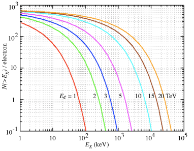
Figure 3: Integral energy spectrum of geo-synchrotron X-rays emitted by 1 TeV to 20 TeV electrons

Figure3 shows the average integral energy spectrum of X-rays emitted by 1$\sim$20 TeV electrons which start isotropically from a height of $3\times 10^{4}$ km and are directed to height 390 km, latitude 0^∘, longitude 130^∘.

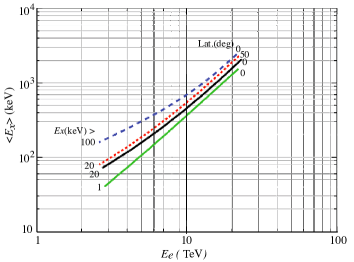
Figure 4: Average energy of X-rays vs electron energy. The minimum X-ray energy is 1, 20, 100 keV as indicated in the Fig. For minimum energy of 20 keV, results for latitude 0^∘ and 50^∘ are shown.

The number of X-rays and the spectrum shape depends on the location. At higher latitudes, in general, a harder spectrum is seen, and the total number of X-rays becomes smaller. However, such differences can be neglected for our present feasibility study, and we use this observation point for further discussions in this article.

In Fig. 4, the average X-ray energy is plotted as a function of the electron energy. The minimum X-ray energy is varied from 1 keV to 100 keV to see the change of the energy dependence. The result for latitude 50^∘ is also shown to illustrate the small difference from the latitude 0^∘ case. For 10 TeV electrons, the average X-ray energy is 600$\sim$700 keV. If the number of X-rays is limited to several, the average generally becomes smaller.

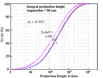
Figure 5: Integral production height distribution of those X-rays that have another X-ray within 50 cm.

The integral production height of X-rays is shown in Fig. 5. We chose those X-rays that have another X-ray within 50 cm. The production height less than 500 km contains 60 % of the events. To judge that X-rays observed are due to the geo-synchrotron emissions, we impose the condition that several X-rays come simultaneously on a line. Since the emission angle of the synchrotron X-rays is order of $\sim 1/\gamma$, the deviation from a line alignment is $\sim$ 2.5 cm for X-rays coming from electrons of energy $E_{e}=10$ TeV at height 500 km. If we impose several X-rays to be aligned in a small distance, lower altitudes with higher magnetic field strength become more important. Therefore, 5 cm is a good measure for the position resolution of the X-ray detector.

In Fig. 6, we show the multiplicity distribution of X-rays falling in an area of 1.4 m$\times 1.4$ m for a primary electron of energy 10 TeV. The minimum energy of X-rays is set to be 40, 60 and 80 keV. In the distribution, we exclude the case where the electron itself enters the area; this is because the electron emits a number of photons by radiation in the detector and they are observed simultaneously at various positions together with the X-rays. This makes it difficult to judge the intrinsic X-rays as discussed later (section 3.3, Fig. 7)

Figure 6: Distribution of X-ray multiplicity in 1.4 m $\times$ 1.4 m area for a primary electron of 10 TeV

3 Consideration of the detector efficiency and backgrounds

For further analysis, we have to assume a model detector and stochastic nature of the observation, together with a background for the observation. Our assumptions are based on a basic test experiment summarized in the Appendix. For example, we put an error to the energy, $E$ (keV), absorbed in BGO by a random sampling with FWHM error of 16$\sqrt{662\ {\rm keV}/E}$ %.

3.1 The tentative detector

The tentative detector is summarized as follows:

1. The unit X-ray detector is made of BGO. The cross-section is 5 cm $\times$ 5 cm and the thickness 2 cm (1.79 r.l; 1r.l = 1.12 cm). Other BGO properties are: density 7.13 g/cm³, light yield 8.2 photons/keV or $15\sim 20$ % of NaI, decay time 300 ns.

2. Each BGO is wrapped in teflon. The top part is covered by CFRP (Carbon Fibre Reinforced Plastic) of 500 $\mu$m thick.

3. The gap between BGO units is filled with thin (1 mm) Sn. Otherwise, a high energy albedo gamma ray could run the small gap rather a long distance and cause multi-Compton scattering which could be a major background.

4. The whole detector size is 1.43 m $\times$ 1.43 m (28 $\times$ 28 BGO’s)

5. Each BGO signal is read by a PMT at the bottom.

6. Simple supporting platform is assumed together with material representing PMT (Fe and glass).

3.2 The observation conditions

We impose the following cuts on each event.

1. We put a threshold, $E_{th}$ on the observed energy, $E_{X}$, in each unit BGO. The standard value of $E_{th}$ is 80 keV. Those BGO’s with observed energy $E_{X}<E_{th}$ are neglected.

2. The number of such BGO units (i.e, $E_{X}>E_{th}$), $m$, must be $\geq 5$. (Of course, we cannot know multiple incidence of X-rays in one BGO and such X-rays are regarded as a single X-ray, though the probability is very small).

3. The energy sum of the two highest energy BGO’s ($E_{1}+E_{2})$ must be $<4.5$ MeV. This is to suppress background events due to multi-Compton scattering of high energy gamma rays.

4. Let the maximum distance among $m-$BGO’s be $d$ cm. The center of each BGO is used to calculate the distance. $d$ is converted to an integer $b$ expressing an effective number of BGO blocks by $(5.1b+5)=d$. We require $b\geq 11$ (See section 3.6.6). Hereafter $b6$ means $b=6$.

3.3 Collection power

One of the merits of observing geo-synchrotron X-rays has been believed to be that we don’t need to observe electrons directly and hence the effective area could be larger than that for direct observation. We define the collection power, $C_{p}$, by

$$C_{p}=\frac{{\rm Number\ of\ events\ with\ a\ desired\ condition}}{{\rm Those\ events\ containing\ the\ electron}}$$ (1)

We note that we must exclude an event which contains the electron itself, since the high energy electron ($>$ TeV) splashes a number of photons to surrounding BGO’s and it becomes difficult to identify synchrotron X-rays (Fig. 7).

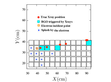
Figure 7: The electron splashes a lot of photons to trigger a number of BGO’s

This fact seems to have been overlooked in past papers, and unfortunately, reduces $C_{p}$ a large amount. If we use a loose cut for observation, $C_{p}$ could be as large as 5, but our condition reduces $C_{p}$ to $<1$. This is partly due to the fact that we require $m\geq 5$; such high multiplicity X-rays tend to be generated near the Earth where the magnetic field is strong, and hence separation of the X-rays and the electron is not large; that means many of the high multiplicity events are accompanied by the electron.

For our observation conditions, events containing the electron are automatically excluded since the energy loss in BGO’s exceeds 18 MeV and $E_{1}+E_{2}>4.5$MeV. In the present paper, we don’t pursue how to utilize such events; if we could find a method for utilizing the events, $C_{p}$ will increase substantially.

3.4 Dependence of observables on electron energy

We use the average of square root of observed energy as a representative of $m-$BGO triggered by X-rays. The energy is in keV unit.

$$\epsilon=<\!\sqrt{E_{X}/\rm{keV}}\!>$$ (2)

The distribution of $\epsilon$ for various electron energies are shown in Fig. 8 for $m\geq 5$, $E_{th}=80$keV, and $b12$ (see 4 in sec.3.2) .

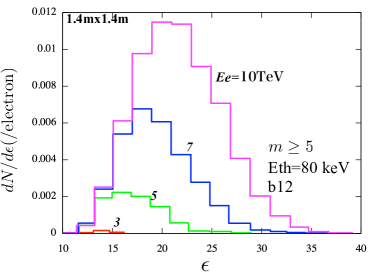
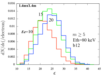
Figure 8: $\epsilon$ distribution satisfying the observation conditions. Upper: for electron energy,$E_{e}=$ 3, 5, 7 and 10 TeV. Lower: $E_{e}=10,15$ and 20 TeV.

The peak position, $\epsilon_{p}$, of each $\epsilon$ distribution and the electron energy are connected roughly by $E_{e}\sim(\epsilon_{p}/10)^{3}$ TeV. The width of the distribution is large ($\sim$ 80 % in FWHM) so that it would be difficult to derive a precise energy spectrum of electrons from those observations.

However, there is a sharp exponential-like cutoff at the high energy side of the synchrotron X-ray spectrum and this gives us, in a sense, the function of a threshold counter to our detector. Actually, we see there is no sensitivity to electrons with energy lower than 2 TeV for the standard cuts. In Fig. 8, each distribution is normalized to give $C_{p}$ when it is integrated. The values are summarized in Table 1.

Table 1: Dependence of $C_{p}$ on electron energy

$E_{e}$(TeV)	3	5	7	10	15	20
$C_{p}$	0.0005	0.018	0.06	0.13	0.18	0.18

3.5 Case study of plausible models

We use 3 models, A, B [1] and C, for the electron energy spectrum in the highest energy region as shown in Fig. 1.

Vela is a good candidate for high energy electron sources. Some models predict that $\sim$ 10 TeV electrons are reaching the Earth. The prediction depends on the distance to Vela, diffusion constant etc. For example, distance dependence is shown in Fig. 1 for 0.25, 0.30 and 0.35 kpc and a diffusion constant of $D=1.0\times 10^{29}(E/$TeV)^0.3cm${}^{2}/$s. An estimate of the probable distance to Vela is 0.25 kpc while the maximum value is expected within $0.39\pm 0.1$ kpc [20]. Since other factors also affect the flux from Vela, we employ here the rather conservative (with respect to flux) distance of 0.3 kpc and use the flux including the contribution from Cygnus Loop. We call this model A. Larger diffusion constants flatten the spectrum. As an example of such a case, we use model B as shown in Fig. 1. Model C is a completely artificial spectrum to examine the detection limit.

The line labeled ’galactic’ is a model calculation [18] which includes distant sources as well as possible near-by sources such as Monogem. The line labeled ’galprop’ is another such model [17] calculated by the Galprop program.

Table 2 shows the integral flux for model A, B and C.

Table 2: Integral flux of model A, B and C: electrons/$\pi$ sr$\cdot$m${}^{2}\cdot$year

	Energy(TeV)
model	$>1$	$>3$	$>5$	$>7$	$>10$	$>15$
A	2248	243	129	74	32.8	8.1
B	3021	324	112	50	18	3.6
C	2080	86	30	14	6	1.6

3.6 Background considerations

When we take an event with $m(\geq$5) synchrotron X-rays aligned, possible backgrounds could come from

1. Chance coincidence of X-rays or charged particles

2. Multiple Compton scattering by a high energy X- or gamma-ray entering the detector

Possible sources of such backgrounds would be

1. Uniform isotropic X-rays and gamma-rays ( Cosmic X-ray Background or CXB)

2. Cosmic ray charged particles such as electrons and protons

3. X-rays from the galactic plane and strong point sources

4. Albedo particles from the earth’s atmosphere

5. A Gamma ray burst

6. Radiation from the environment surrounding the detector

7. South Atlantic Anomaly Radiation

8. A Solar flare

As to the environmental radiation, we must choose a low background environment and, this is expected to be possible owing to our observation conditions. The last two sources might be avoided by switching off the electronics. If a gamma ray burst is as strong as triggering more than 5 BGO’s almost on a line in a short time (10 ns; see later), we could get information from other GRB observatories.

Next, we summarize other factors and derive the chance coincidence rate.

3.6.1 Cosmic X-ray Background: CXB

CXB (Diffuse X-rays) is now well understood and we can calculate the background due to CXB. The background by other sources is estimated as the ratio to the one for CXB. As the low energy CXB, we use the data from HEAO-I [21] which was confirmed by Swift/BAT [22] recently. The data can be continued to the SAS-2 [23] and EGRET [24][25] data at higher energies (Fig. 9).

Chance coincidence by CXB must be considered at low energies ($<500$ keV). As to low energy electrons and protons, their flux [27][28] is much lower than CXB and we don’t need to consider their effect. Also it’s difficult for high energy charged particles to generate BGO signals on a line with energy deposit less than a few MeV which is our maximum cut.

Table 3: Flux of CXB: the 3rd line shows the integral flux over $E_{X}$(in $\pi$sr)

$E_{X}$ (MeV)	0.01	0.02	0.03	0.04	0.05	0.06	0.07	0.08	0.1	0.2
/cm2s sr MeV	316	102	42.2	25.6	15.0	9.3	6.15	4.33	2.43	0.417
/cm2s	10.7	5.18	3.12	2.09	1.47	1.10	0.86	0.704	0.5	0.175

0.3	0.5	1	2	5	10	20	50	100
0.15	0.042	7.4(-3)	1.4(-3)	1.5(-4)	2.8(-5)	5.9(-6)	7.9(-7)	1.6(-7)
0.096	0.045	1.69(-2)	6.6(-3)	1.75(-3)	7.2(-4)	3.08(-4)	1.01(-4)	4.5(-5)

3.6.2 Atmospheric albedo particles

High flux low energy particles which might contribute to chance coincidences can be absorbed by the support structure to be put on the Earth side. High energy particles are not able to make fake events by multi-Compton scattering. However, X-rays and gamma rays in the intermediate energy region must be considered. Their angular distribution and latitude dependence are rather complex. At high energies ($>30$ MeV), there are data from SAS-2 [29] and EGRET [30]. In the X-ray energy region, recent reliable observations from Swift/BAT [22] show a steeper spectrum and thus a higher flux in the low energy region ($<200$ keV) than the older one [31].

Figure 9: Energy spectra of the isotropic diffuse X/gamma-rays (CXB) and atmospheric albedo X/gamma-rays.

Although there is a maximum of 5 times difference in the fluxes around the equator and magnetic poles, the over all difference is within a factor of 3. We smoothly connect Swift/BAT data averaged over latitude and SAS-2($\sim$ 30 MeV) and EGRET ($\sim$ 100 MeV) data. Figure 9 shows the energy spectra of CXB and albedo X/gamma-rays which we used in the simulation. At the high energy side, the albedo flux is much higher than CXB. Since the atmospheric albedo is complex, we use, for safety, an overestimated flux if there are uncertain factors.

From this point of view, we employ a 1.5 times higher flux than Swift/BAT data in Fig. 9. We also assume that the Swift/BAT data is the flux from the Nadir direction (this will probably lead to overestimation of the background). If we measure the X/gamma-ray angle $\theta$ from the Nadir, the Earth horizon is at $\theta\sim 70^{\circ}$ where the albedo flux becomes maximum. This enhancement effect can be well modelled by assuming that the angular distribution of X/gamma-rays which enter the bottom side of the detector is not $\cos\theta d\cos\theta$ but $d\cos\theta$ (i.e, not isotropic but there is $\sim\sec\theta$ enhancement).

With this assumption, if we compare the all angle intensity of the albedo over 80 keV to CXB without considering absorption by the structural material, we get albedo/CXB $\sim 4$. If we assume a supporting material equivalent to Pb 500 $\mu$m or Fe 1 mm, the albedo flux becomes 1.29 (/cm${}^{2}\cdot$s) or 2.15 (/cm${}^{2}\cdot$s), respectively. The ratio to CXB reduces to $\sim 1.8$ or $\sim 3.1$, respectively. However, we don’t consider this absorption effect for albedo for the moment.

3.6.3 X-rays from the galactic plane

The X-ray intensity per unit solid angle from the galactic plane is factor $\sim$10 stronger than CXB. However, what is important for the chance coincidence is the integral value over a hemisphere. Its ratio to CXB is considered to be almost constant above 10 keV to over 10 MeV. This ratio is estimated to be less than 0.1 by Ginga[32] and ASCA[33]. This value is for the case when the galactic plane is near the zenith. Therefore, we can safely neglect X-ray contribution from the galactic plane as compared to albedo or CXB.

3.6.4 Chance coincidence

We first consider the chance coincidence by CXB; we estimate background events with $m$ X-rays aligned. The factors to be considered are

• Time resolution of the system. $\tau$ in FWHM.

• Effective flux over 80 keV. $f$

• Area where the X-rays there can be regarded as on a line. $\Delta S$

• The total area of the detector. $S$.

• Observation time. $T$.

• X-ray multiplicity. $m$.

Then, the number of chance events, $N$, in the observation time is

$$N\sim fST(f\Delta S2\tau)^{m-1}$$ (3)

Expressing $\tau$ in ns, area in m², $T$ in year and $f=\alpha f_{0}$ where $f_{0}=0.704$/cm${}^{2}\cdot$s is the CXB integral flux over 80 keV (we call $\alpha$ effective background index), we obtain

$$N\sim 2.18\alpha ST(\alpha\Delta S\tau)^{m-1}(1.408\times 10^{-5})^{m-1}\times 10^{11}$$ (4)

For $S=2$, $\Delta S=0.2$, $T=1$, $m=5$,

$$N\sim 2.74\times 10^{-11}\alpha^{5}\tau^{4}$$ (5)

This relation is shown in Fig. 10

Figure 10: The number of chance coincidence events, $N$, as a function of time resolution ($\tau$) and effective background index($\alpha$) for $S$=2m², $T=1$ year．

As described later, we found $\tau=5.4$ ns with use of a constant fraction discriminator; this value is realistic even at 80 keV but we assume here $\tau=$10 ns for safety. The maximum possible value of $\alpha$ would be

$$\alpha=1(\rm{CXB})+4(\rm{albedo})+0.1(\rm{galactic\ plane})\sim 5$$

Then, we can expect the number of chance coincidence events is $\ll 0.01$ for a 1 year observation. As the condition for line alignment, we use only the $\Delta S$ constraint, so the actual background could be reduced.

3.6.5 Background by multi-Compton scattering

A gamma-ray may repeat a Compton scattering in BGO and/or environmental media and can make a fake event as if synchrotron X-rays are on a line. Due to the condition, $m\geq 5$, the energy of such a gamma-ray is concentrated in $5\pm 3$ MeV and very seldom exceeds 25 MeV.

If we require $m\geq 5$ and the maximum distance between the triggered BGO’s be greater than 30 cm, we may expect a very small number of fake events. However, the number of CXB over 1 MeV entering 2 m² area in one year exceeds $10^{10}$ while expected signal is order of $10\sim 20$ events. Then, we have to consider an event with probability of $\sim 1/10^{9}$.

We first calculate multi-Compton event rate using CXB, and the contribution from albedo is considered by introducing the effective ratio $\displaystyle\alpha^{\prime}=\frac{albedo}{CXB}$

Multi-Compton events are efficiently produced by $\sim$ 5 MeV gamma-rays. The albedo gamma-rays in this energy range are $\sim 40$ times more abundant than CXB. Albedo from the Earth horizon have a nadir angle of $\theta\sim 70$ degrees and are apt to produce multi-Compton scattering events. Therefor, it would be appropriate to take $\alpha^{\prime}\sim 40\times 3\pi/4\sim 100$ for safety.

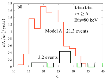
Figure 11: $\epsilon$ distribution by model A and background for one year observation. The background rapidly reduces as $b$ increases. Top: $b6$, background dominates. next: $b8$,$b9$, bottom: $b10,11,12$. background vanishes but signal remains almost the same.

3.6.6 Signal vs background

To show how the aligned X-rays are widely spanned, we use, for example, $b10$ as defined in 4 in section 3.2.

Figure 11 shows signal vs background for model A under the condition of $S=2$m², $E_{th}=$80 keV, $m\geq 5$ for various $b$. The CXB background for $b9$ becomes $\sim 0.2$ but if the albedo effect is to be included, $\alpha^{\prime}$ must be multiplied and the background becomes quite comparable to the signal ($\sim 20$ events). The signals for b10 to b12 do not change appreciably, while background decreases faster than exponential and for b10,11,12 it becomes $\sim$0.02, 0.001, $\ll\!0.001$. Therefore, with b11 or b12, we can completely neglect the background from albedo multi-Compton scattering.

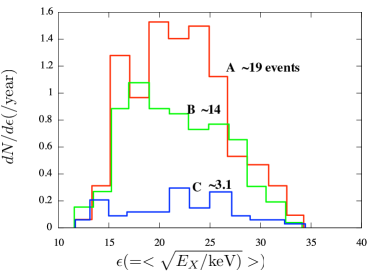
Figure 12: Comparison of expected signals by Model A, B and C

Figure 12 compares the case of Model B and C with Model A (b12). The number of expected events for Model B is $\sim 14$; it’s smaller than model A ($\sim 19$) but within the detectable range. The smaller number reflects the difference of the spectrum shape, but it would be difficult to derive the original spectrum shape. Artificial model C gives $\sim 3.2$ events in a year. This gives a reference of the minimum detectable flux; we would be able to say that a model is plausible or incompatible with the observation only if the flux is much higher than $1.5\times 10^{-8}(E$/2.3TeV)^-3(/m²s sr GeV) over 2 TeV.

3.6.7 Light/thermal shielding and pile-up effect

In this trial calculation, we assume X-rays with more than 80 keV energy. However, we must prevent a pile-up effect in BGO due to lower energy X-rays. CFRP is supposed for light/thermal shielding, and if we make its thickness to be 500$\mu$m (0.11g/cm²) carbon equivalent, we obtain the X-ray transmission rate as shown in Table 4.

Table 4: X-ray absorption by 500$\mu$m carbon

$E_{x}$ (keV)	3		5		10		60		100
incident angle (deg)	0	70	0	70	0	70	0	70	0	70
transmission rate(%)	$0.0012$	0	25	1.5	75	43	98	95	98	95

CXB over 3 keV is expected in a 5 cm $\times$ 5 cm area at $\sim$400 Hz, but those photons reaching the BGO are less than 100 Hz. Low energy albedo has much smaller flux than CXB, as in Fig. 9. Supposing the effective flux of albedo over 80 keV is 4 times CXB, then the rate of each BGO is $\sim 70$ Hz. Therefore, X-rays entering each BGO will not exceed 200 Hz in normal conditions. This means pile-up in BGO dose not matter since the decay time of BGO light emission is $\sim 300$ ns.

3.6.8 Trigger rate and dead time

Trigger rate will be governed by multi-Compton scattering. According to the simulation, the CXB contribution with the condition of any 3 BGO coincidence ($E_{X}>80$keV) is $\sim$1Hz, and for any 4 coincidence $\sim$0.045Hz. The albedo will contribute a maximum of 100 times of this and will make $\sim$100Hz for any 3 and $\sim 4.5$ Hz for any 4 coincidence, respectively. Our target is $m\geq 5$, however, any 4 coincidence trigger will be appropriate.

Since the decay time of BGO light is $\sim$ 300 ns, we may assume $\sim 1$ ms dead time. Then, the trigger rate of $\sim$10 Hz presents no problem.

4 Summary and concluding remarks

• The purpose of this article is a study of the feasibility of probing cosmic ray primary electrons in the $\sim$10 TeV region by observing geo-synchrotron X-rays. According to some plausible models, such high energy electrons are expected to come from supernova remnants such as Vela.

• For this, we assumed a tentative detector design consisting of a number of BGO blocks as described in 3.1

• It is found that we cannot use events which contain the electron itself falling on the detector; a high energy electron splashes a number of X/gamma-rays and thus it is difficult to identify aligned X-rays. This reduces event the rate substantially.

• To realize a background free observation, the number of triggered BGO’s (with X-ray energy$>$ 80 keV) must be $m\geq 5$ and they must span more than 62 cm.

• It will be difficult to get a spectrum shape for electrons. However, owing to the exponential sharp cut-off of the X-ray energy spectrum for each electron energy, the assumed detector has no sensitivity to electrons below 2 TeV, and thus works like a threshold detector.

• We can verify the plausibility of models if the flux is much (4$\sim$5 times) higher than $1.5\times 10^{-8}(E$/2.3TeV)^-3(/m²s sr GeV) over 2 TeV. The number of signal events is expected to be 15 to 20 in a year.

• It will be possible to increase the number of signal events by lowering the threshold for observation down to $sim$50 keV without a big problem (chance coincidence is still negligible and multi-Compton scattering event rate is not affected). Then, the number of signal events will double or the detector could be made smaller.

• Lowering $m$ by 1 is very challenging because the chance coincidence probability increase substantially. However, in our calculation we only considered $\Delta S$ for a line alignment constraint. This is a loose condition rather than a rigorous one. Also we may note that $\epsilon$ by chance coincidence distributes sharply at the lower end of the true signal distribution. This is useful to separate some of the true signal. These factors are worth further consideration.

• The observation considered here would be more attractive if it could be combined with gamma-ray burst observations.

Appendix A Basic test of detector components

To get basic performance of assumed detector components, we performed the following basic test experiments. The parameters thus obtained were used in the present calculations.

A.1 Materials

• BGO (SICCAS):

  5cm$\times$5cm$\times$2cm t block $\times 8$. As reflector, white teflon was used. Thin CFRP was used for light/thermal shield.

• PMT (Hamamatsu):

  R3318-HA(bialkali, 2”square) $\times 2$.
  R6231-100HA(super bialkali, 2”$\phi$) $\times 2$

  To see possible individual differences, two PMT’s were used for each type.

• X and gamma-ray source

  ²⁴¹Am(60keV, 14 keV), ⁵⁷Co(122keV), ¹³⁷Cs(662 keV), ⁶⁰Co(1.17 MeV, 1.33MeV)

A.2 Temperature dependence

To avoid a temperature dependence in the test, and for future applications, we examined the temperature dependence of pulse height for the complete absorption peak of 662 keV gamma-rays.

At 15 to 30^∘ C, temperature dependence of BGO is within $\sim\pm 2$%. At lower temperatures down to -30^∘C, $\sim-0.5$%/deg dependence is seen. Therefore, the temperature effect is negligible in our test conducted at room temperatures. LaBr3 has only $\sim\pm 2$% changes over the entire range.

A.3 Energy resolution

We exposed isotope sources mentioned in A.1 to the BGO’s to obtain pulse height distributions. Except for 60 keV X-rays from ²⁴¹Am, data was taken for all combinations of 3 sources, 8 BGO blocks and 4 PMT’s (total 96 cases).

The maximum difference of energy resolution (in FWHM) among 8 BGO’s is 4% for 662 keV and 7% for 122 keV. So we need to choose good BGO for low energy X-ray observation in actual application. Two PMT’s, Bialkali (B) or Super Bialkali (SB), show only a small difference (within 2%). SB gives $\sim 2$ % better resolution than B for 662 keV and $\sim 4$% for 122 keV. The SB PMT recognized clearly two peaks at 1.17 MeV and 1.33 MeV gamma-rays from ⁶⁰Co, but the B PMT showed no clear separation.

This difference is reasonable considering the maximum yield wavelength (480 nm) of BGO, wave length dependence of the quantum efficiency and differences in light collection efficiency due to the square and circular PMT areas.

Figure 13: Energy dependence of energy resolution (% of FWHM). The results for SB PMT voltage of 900 V and 1000 V are shown. Accuracy of points with () is less than other points due to difficult background subtraction. The point at $\sim 33$ keV is estimated from a peak obtained in ⁵⁷Co case (Note: the K-shell energy of Bi is 90.5 keV and ⁵⁷Co has $\sim$11% 136 keV line besides its 122 keV line. We expect a line near $(123.5-90.5)$ keV. ). The curve shows the resolution, $16\sqrt{662\ \rm{(keV)}/E})$ %, used in the simulation to put a random error on the absorbed energy in BGO.

Figure 13 shows SB PMT measurement results. A difference of $\sim$3 % does not matter for our purpose and, in the simulation, we assumed a resolution shown by the curve in the figure to introduce a random error to the absorbed energy in BGO.

A.4 Dynamic range

Dynamic range of the PMT was examined by applying voltages from 850 to 1000 V. The pulse height is linear as a function of X-ray energy from 14 keV to 1.25 MeV, except for 850 V case for which linearity is lost in the 10 keV region (it is difficult to see the 14 keV peak). Voltage dependence of the pulse height is $\propto V^{5.6}$ for each energy. Since our target is 50 keV to few MeV, this feature will make it easy to build electronics.

A.5 Time resolution

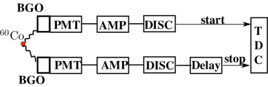
Figure 14: Setup for measuring time resolution of the BGO+PMT system

To avoid chance coincidence, good time resolution is indispensable. To see the time resolution, we use a system as shown in Fig. 14 and measured time difference, $\Delta T$, from start to stop. Two gamma rays from ⁶⁰Co (1.17 and 1.33 MeV) are emitted isotropically and simultaneously and will enter BGO at the same time. In some cases, one gamma-ray which enters a BGO block may be Compton scattered and enters another BGO. This timing is also the same within our accuracy.

Figure 15: Time difference distribution observed in the setup shown in Fig. 14. One channel is 50 ps. The constant fraction method gives 5.4 ns FWHM resolution, while the leading edge method gives 9.1 ns, and the distribution has a long tail deviating from Gaussian.

To get good resolution, we use a constant fraction discriminator (ORTEC 935). We also use a leading edge discriminator to confirm the merit of using the constant fraction method as seen in Fig. 15

The pulse height from 1.2 MeV absorption is $\sim$ 100 mV, and we use a discrimination level of 50 mV. For timing, 50% fraction is used. The data include Compton events which have smaller energy than 1.2 MeV; thus the result indicates similar good time resolution even for smaller energy deposit. To see this, we use the discrimination level of 25 mV and 10 mV to find less than 1 ns degradation of the time resolution. This suggests 10 ns resolution is quite safe for several tens keV region.

References

- kobayashi et al [2004] T. Kobayashi et al.,APJ, 601:340?351, 2004 January 20.
- Aharonian et al [2008] F. Aharonian et al. [H.E.S.S. Collaboration], Phys. Rev. Lett. 101 (2008) 261104.
- Aharonian et al [2009] F. Aharonian et al. [H.E.S.S. Collaboration], arXiv:0905.0105 [astro-ph.HE].
- Torii et al [2007] For example, S.Torii, et al., 30th ICRC (Mexico), OG1.5, 2007.
- Veronica [2010] For example. B. Veronica, NIM A, 617,1-3,pp462-463 (2010)
- Prilutskii [1972] O. F Prilutskii, Sov. Phys. JETP Lett., 16, 320, 1972
- McBreen [1977] B. McBreen, Proc. ESLAB Symp., 12th, 319, 1977
- Stephens et al [1983] A.E. Stephens and V.K. Balasubrahmanya, J. Geophy. Res.88, A10,7811(1983).
- Nahee et al [2010] P.Nahee et al [CREST collaboration], 38th COSPAR Scientific Assembly. Held 18-15 July 2010, in Bremen, Germany, p.2; Also S. Nutter et al. Proc. of 31st International Cosmic Ray Conference, Lodz, Poland, 2009.
- Abdo et al [2009] A. Abdo et al. [Fermi-LAT Collaboration], Phys. Rev. Lett. 102 (2009) 181101.
- Chang et al [2008] J. Chang et al. [ATIC Collaboration], Nature 456 (2008) 362
- Aguilar et al [2002] M. Agullar et al., Phys. Reports 366 (2002) 331
- kobayashi et al [1999] T. Kobayashi et al. 1999, Proc. 26th Int. Cosmic-Ray Conf. (Salt Lake City),203, 61
- DuVernois et a [2001] M.A. DuVernois et al. [HEAT Collaboration], ApJ 559 (2001) 296
- Torii et al [2001] S. Torii et al [BETS group] APJ, 559, (2001), pp. 973-984.
- Torii et al [2008] S. Torii et al., [PPB-BETS Collaboration], arXiv:0809.0760 [astro-ph].
- Grasso et al [2009] D. Grasso et al, Astroparticle Physics 32 (2009) 140–151.
- Strong et al [2004] A.W. Strong, I.W. Moskalenko, O. Reimer, ApJ 613 (2004) 962.
- Baring [1988] M. Baring, Mon. Not. Astr. Soc., 235 (1988).
- Alexandra [1999] N. Alexandra et al. APJ, 515:L25–L28, 1999 April 10.
- Gruber et al [1999] Gruber et al., APJ,520:124-129, 1999 July 20.
- Ajeloo et al [2008] M. Ajello, et al., APJ, 689:666–677(2008).
- Fichitel et al) [1977] C.E.Fichitel et al., APJ, 217, L9-L13,1977.
- Kniffen et al [1996] D.A. Kniffen et al., Astronomy and Astrophysics, Suppl. 120, 615-617(1996).
- Strong et al [2004] A. W. Strong, I. V. Moskalenko, and O. Reimer, APJ 613, 956 (2004).
- Abdo et al [2010] A.Abdo et al [Fermi-LAT collaboration], Phys. Rev. Lett..,104, 10, id. 101101.
- Huston et al [1998] S.L.Huston and K.A.Pfitzer, Space Environment Effects: Low-Altitude Trapped Radiation Model. NASA/CR-1998-208593.
- Armstrong et al [2000] T.W. Armstrong and B.L. Colborn, Trapped Raditaion Model Uncertainties: Model–Data and Model–Model Comparisons. NASA/CR-2000-210071.
- Thompson et al [1981] D. J. Thompson, G. A. Simpson and M. E. Ozel, Journal of Geophysical Research, 86, No. A3, March 1, (1981)pp.1265-1270.
- Petry et al [2005] Dirk Petry et al, arXiv:astro-ph/0410487v1. AIP Conference Proceedings, 745. New York: American Institute of Physics, 2005., pp.709-714
- Imhof et al [1976] W. L. Imhof, et al., Journal of Geophysical Research. 81, no. 16 june 1, 1976.
- yamasaki et al [1997] N.Y. Yamasaki et al., APJ, 481:821-831, 1997 June 1
- Tanaka et al [2002] Y.Tanaka, A&A 382, 1052-1060 (2002).
- Hunter et al [1997] S. D. Hunter et al., APJ, 481:205-240, 1997 May 20