Making ARPES Measurements on Corrugated Monolayer Crystals: Suspended Exfoliated Single-Crystal Graphene

Abstract

Free-standing exfoliated monolayer graphene is an ultra-thin flexible membrane, which exhibits out of plane deformation or corrugation. In this paper, a technique is described to measure the band structure of such free-standing graphene by angle-resolved photoemission. Our results show that photoelectron coherence is limited by the crystal corrugation. However, by combining surface morphology measurements of the graphene roughness with angle-resolved photoemission, energy-dependent quasiparticle lifetime and bandstructure measurements can be extracted. Our measurements rely on our development of an analytical formulation for relating the crystal corrugation to the photoemission linewidth. Our ARPES measurements show that, despite significant deviation from planarity of the crystal, the electronic structure of exfoliated suspended graphene is nearly that of ideal, undoped graphene; we measure the Dirac point to be within 25 meV of $E_{F}$. Further, we show that suspended graphene behaves as a marginal Fermi-liquid, with a quasiparticle lifetime which scales as $(E-E_{F})^{-1}$; comparison with other graphene and graphite data is discussed.

I Introduction

The recent availability of monolayer-thick two-dimensional crystals such as graphene, BN, and BSCCO has generated widespread interest in the physics and materials science communities. In the case of graphene, in particular, the two dimensional nature of the crystal in combination with its unusual massless Dirac fermions determines a host of intriguing and unique transport phenomena, including graphene’s half-integer quantum Hall effect (HE) and non-zero Berry’s phase.Novoselov et al. (2005); Zhang et al. (2005) Unlike most metals, undoped graphene has a Fermi surface which consists of a set of 2 inequivalent points in momentum-space. Thus, at zero temperature and zero doping, the density of states at the Fermi level vanishes. In combination with the linear dispersion of low energy charge carriers, this vanishing density of states is expected to lead to unusual band-renormalization effects that are not seen in Fermi-liquid systems such as unusually high electron-electron coupling. Motivated by interest in these unusual properties, several theoretical and experimental studies have investigated the electronic properties of graphene.Neto et al. (2009)

Angle-resolved photoemission spectroscopy (ARPES) is the experimental method that is most frequently used to probe the electronic structure of crystals. However, so far, the majority of ARPES studies of graphene have been conducted on epitaxial graphene, which has been grown on a variety of substrates such as SiC, Ru, Ni and Ir. Ohta et al. (2006); Bostwick et al. (2006); Dedkov et al. (2008); Shikin et al. (2000); Vázquez de Parga et al. (2008); Liu et al. (2010); Pletikosić et al. (2009); Sutter et al. (2009) Epitaxial graphene is ideal for photoemission experiments, but, due to the interaction between the epitaxial graphene monolayer and the substrate, the band structure is often distorted such that the Dirac point shifts away from the Fermi energy, thus changing the quasiparticle dynamics. In an effort to minimize the effect of substrate interaction on epitaxial graphene, recent ARPES studies have focused on several multilayer systems, such as intercalated graphiteValla et al. (2009) and graphene grown on the C face of SiC. Sprinkle et al. (2009) These layered systems consist of multiple stacked graphene sheets that are substantially electrically isolated, thus resulting in an electronic band structure that mimics that of suspended exfoliated single-layer graphene. However, despite its scientific and technological importance, exfoliated graphene has been the subject of only a limited number of ARPES studies,Knox et al. (2008); Liu et al. (2010) despite the fact that it remains the best choice for device physics, as it is easily backgated and has the highest measured mobility.Bolotin et al. (2008)

Several obstacles impede measurement of the bandstructure of exfoliated graphene. One difficultly arises from the fact that available single-layer exfoliated graphene flakes are typically less than 20 $\mu$m in size, thus precluding the use of standard ARPES systems, which require samples to be several mm in size. Hence, most information regarding low-energy occupied states in exfoliated graphene has been obtained indirectly from electrical-transport measurementsNovoselov et al. (2005); Zhang et al. (2005) or directly by optical-probing techniques.Wang et al. (2008); Mak et al. (2010) These techniques examine the bandstructure generally within  1eV of the Dirac point and do not directly provide momentum resolution. For photoemission the limitation in size can be overcome by working with high lateral-spatial-resolution probes such as those available using spectromicroscopy.Fujikawa et al. (2009); Sutter et al. (2009) A second major impediment to photoemission studies is due to the fact that graphene is an ultrathin crystal. This ultrathin property has, in turn, two important consequences for photoemission studies. The first is the transparency of monolayer graphene to UV photons and photoemitted electrons, which causes a strong background photoemission signal if the monolayer graphene is in close physical proximity with a substrate.Knox et al. (2008) The second is that exfoliated graphene is not atomically flat, but is known to deform locally, a result shown through AFM, STM, electron microscopy, and electron scattering results.Geringer et al. (2009); Ishigami et al. (2007); Locatelli et al. (2010); Stolyarova et al. (2007); Cullen et al. (2010) It has been argued that the deformation is due to the fact that monolayer-thick graphene has soft flexural modes leading to ready bending of the graphene. The presence of a supporting substrate or scaffold can, to a certain degree, stabilize height fluctuations in the graphene layer, but corrugations in the underlying supporting substrate are transferred in part to the graphene due to the reduced stiffness of this material. Additionally, intrinsic corrugations that cannot be attributed to interaction with the substrate were recently observed in supported graphene.Geringer et al. (2009) Further, in a recent low energy diffraction study, we demonstrated that even graphene suspended over etched cavities exhibits corrugation, which appeared to have been intrinsic in origin. Locatelli et al. (2010)

Thus, in general, two dimensional crystals produced by exfoliation may show significant local curvature, manifested as corrugation and ripples. This corrugation is known to affect not only the electronic and transport properties of the material, but can also have a major impact on photoemission results. In particular, the theory of ARPES was developed for single-crystal atomically flat surfaces and relies on the fact that momentum perpendicular to the surface is conserved in the photoemission process. On such perfectly ordered crystals the photoemission lineshape is directly related to the spectral function of the electronic state being probed, from which information about many-body physics can be extracted. The corrugation in thin sheets of layered materials breaks this symmetry and obscures the intrinsic many-body effects.

In this paper, we present a systematic approach to account for such corrugation-induced broadening in ARPES on thin films. By combining our photoemission results with detailed information about surface morphology obtained from prior electron-microscopy measurementsLocatelli et al. (2010) taken in-situ on the same samples we are able to quantify the influence of corrugation on spectral broadening. We go on to describe a method to discount the effect of surface corrugation from ARPES measurements to reveal the intrinsic many-body physics present in graphene. Our results show that suspended graphene behaves as a marginal Fermi-liquid with an anomalous quasiparticle lifetime which scales as $(E-E_{F})^{-1}$.

II Experiment

Our measurements used the Spectroscopic Photoemission and Low Energy Electron Microscope (SPELEEM) at the Nanospectroscopy beamline at the Elettra Synchrotron light source.Locatelli et al. (2003) The SPELEEM is a versatile multi-technique microscope that combines low energy electron microscopy (LEEM) with energy-filtered X-ray photoemission electron microscopy (XPEEM). The microscope images surfaces, interfaces and ultra-thin films using a range of complementary analytical characterization methods, which have been described in detail previously. Schmidt et al. (1998); Locatelli and Bauer (2008) When operated as a LEEM, the microscope probes the specimen using elastically backscattered electrons. LEEM enables high sensitivity to surface crystalline structure and, due to the favorable backscattering cross-sections of most materials at low energies, allows image acquisition to be obtained at video frame rate. The lateral resolution of the microscope for LEEM imaging is currently below 10 nm. In XPEEM mode, the specimen is probed using the beamline photons, provided by an undulator source; thus, the technique is sensitive to the local chemical and electronic structures. Laterally resolved versions of synchrotron based absorption (XAS) and photoemission spectroscopy (XPS) are possible. The lateral resolution in XPEEM approaches a few tens of nm.Locatelli et al. (2006)

Along with real-space imaging, the SPELEEM microscope is capable of micro-probe diffraction imaging, i.e. laterally restricted low energy electron diffraction ($\mu-$LEED) and angle resolved photoemission electron spectroscopy ($\mu-$ARPES) measurements when probing with electrons and photons, respectively. In diffraction operation the microscope images and magnifies the back focal plane of the objective lens. In ARPES mode, the full angular emission pattern can be imaged on the detector up to a parallel momentum of $\sim 2\text{\AA}^{-1}$; at larger parallel momentum the transmission of the microscope decreases. All diffraction measurements are restricted to areas of $\sim$ 2 $\mu m$ in diameter, which are selected by inserting a field limiting aperture into the first image plane along the imaging-optics column of the instrument. Thus, the microscope enables measurements on samples that are homogeneous over areas of a few square microns. The energy resolution of the SPELEEM in diffraction imaging, such as ARPES and photoelectron-diffraction measurements, is 300 meV and the transfer width of the microscope when operated in LEED mode is 10 nm.

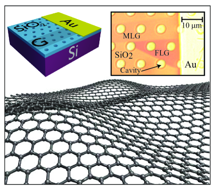
Figure 1: (Color Online) (Left) Schematic drawing of our suspended-graphene sample configuration. (Right) Optical micrograph of sample containing suspended monolayer graphene (MLG) and few-layer graphene (FLG). (Bottom) Artists rendering of corrugated graphene crystal (height fluctuations not to scale).

Graphene samples were extracted by micro-mechanical cleavage from Kish graphite crystals (Toshiba Ceramics, Inc.) and placed onto an SiO₂-thin-film layer on an Si substrate, which was previously patterned with cylindrical cavities to a depth of 300 nm, as described in Ref. Locatelli et al., 2010. The use of planar processing of this substrate allowed us to suspend areas of the graphene films without the use of further photolithographic techniques, which would introduce contaminants to the graphene sheets. Graphene samples with lateral sizes from 10 to 50 $\mu$m were placed in contact with Au grounding strips deposited on the surface via thermal evaporation through a shadow mask. A sketch of the sample configuration is shown in Fig. 1 along with an optical micrograph.

The SPELEEM instrument used to collect data has the important advantage of having a sufficiently high spatial resolution to guarantee that we are measuring a single crystal sample of monolayer graphene and that all of the measured spectral intensity is derived from a fully suspended region. This capability is necessary since the suspended regions are approximately 5 $\mu$m in diameter and, therefore, cannot be resolved with conventional photoemission instruments, which employ spatial averaging techniques that collect data over surface areas of several square millimeters. The potential to combine both photoemission and electron scattering measurements is essential for our experiment since it allows us to measure bandstructure and surface morphology on the same samples. We note, additionally, that a similar instrument was recently used in a study, which examined the morphology and electronic structure of epitaxial graphene grown on Pt.Sutter et al. (2009)

After preparation the samples were placed into a UHV chamber with a base pressure of $2\times 10^{-10}$ mbar, and the surface cleaned via low energy electron irradiation to eliminate adventitious hydrocarbon molecules adsorbed during prior atmospheric exposure.Locatelli et al. (2010) All graphene samples were characterized with LEEM before investigation with ARPES and LEED. For each sample, LEEM was used to locate sample areas of interest and to determine film thickness with atomic resolution by measuring intensity modulations in the LEEM I-V spectra.Locatelli et al. (2010); Hibino et al. (2008); Altman (2005)

ARPES data at multiple photon energies were obtained on the suspended areas of the graphene film. Only regions of uniform thickness were considered. In order to elucidate the role of surface corrugation and substrate influence, comparative experiments were also carried out on corresponding regions where the film was supported by the SiO₂ substrate. This surface has been recently carefully calibrated by prior STM and electron-scattering measurements. Ishigami et al. (2007); Stolyarova et al. (2007); Geringer et al. (2009) In addition, ARPES measurements were made on Kish-graphite flakes that were present on the same substrates. As graphite is a well understood and commonly studied system, these measurements provided a useful point of comparison for our graphene measurements. Photoemission from graphite is, in some respects, similar to that from graphene because of the stacked-layer nature of the former. However, the physics near the Dirac point is significantly different owing to the fact that the multilayer stacking in graphite breaks the symmetry between A and B sublattices, which results in two dispersing branches, such that low energy excitations do not have the simple linear dispersion relation that is found for graphene.

III Results

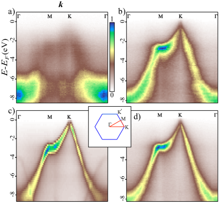
Figure 2: (Color online) Raw ARPES data along symmetry directions in Brillouin Zone for graphene and graphite. (a)SiO₂ supported graphene ($\hbar\omega$=90 eV). (b) Suspended graphene ($\hbar\omega$=84 eV). (c)Kish graphite ($\hbar\omega$=90 eV). (d) Suspended graphene ($\hbar\omega$=50 eV). Inset shows 2D graphene Brillouin zone.

Photoemission spectra were measured from two samples with differing degrees of surface corrugation and substrate interaction, that is, on suspended and substrate-supported graphene. Previous LEED measurements have shown that the horizontal correlation length increases from 24 nm to 30 nm in measurements taken on supported and suspended samples, respectively.Locatelli et al. (2010) In addition, ARPES data were collected at room temperature over the entire surface Brillouin zone (SBZ) from 0.5 eV to -8 eV (energy referenced to $E_{F}$), for monolayer graphene and graphite, using a range of photon energies. Figure 2 shows ARPES spectra taken from a sample supported by and in contact with the SiO₂ surface and a sample that was suspended over the 5 $\mu$m wells shown in Fig. 1. For comparison, the raw ARPES spectrum from Kish graphite is shown as well. The data show dispersion along 3 symmetry lines in the SBZ. As expected from the reduced corrugation, as well as the absence of any substrate interaction, the ARPES data for suspended graphene show a dramatic improvement in quality as compared to the data for supported graphene. Additionally, there is a very broad, parabolically dispersing peak centered at the $\Gamma$ point at a binding energy of $\sim$8 eV in the data taken on supported graphene. This feature has been previously attributed to photoemission from the amorphous SiO₂ substrateKnox et al. (2008) and is not observed in the spectrum taken on suspended graphene. Although the substrate is only 300 nm below the suspended graphene, any background electrons emmited at this height will be significantly defocused in the electron optics of SPELEEM microscope. Additionally, due to the grazing incidence angle of the photon beam (16^∘), the bottom of the cavity is not fully illuminated as the cavity edge casts a shadow, which further reduces the photoemission signal from the substrate.

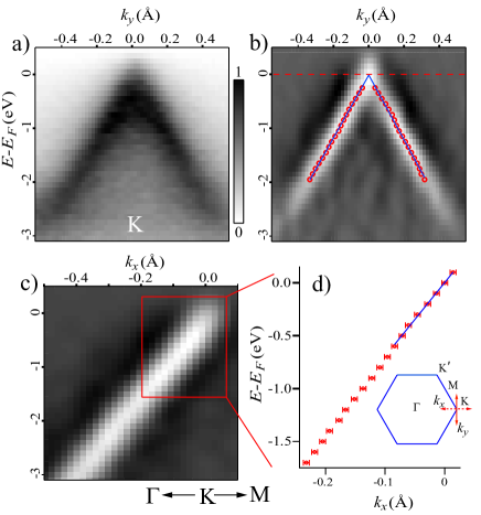
Figure 3: (Color online) (a) ARPES intensity through K point along $\Gamma$M ($k_{y}$) direction in suspended monolayer graphene ($\hbar\omega=50eV$). (b) Smoothed second derivative image of dispersion shown in (a). (c) Smoothed second derivative ARPES intensity through K point along $\Gamma$K ($k_{x}$) direction. (d) Extracted dispersion from (c) Inset shows graphene Brillouin zone. Red solid (dashed) line indicates $k_{y}$ ($k_{x}$) direction through K point.

In the vicinity of the K points, a conical dispersion is observed centered at the K point on the suspended graphene spectrum. At $\sim 1$ eV below the Fermi level a trigonal-warping deviation from angular isotropy becomes clearly noticeable. Measurements taken through the K point and in the direction parallel to the $\Gamma$M direction (vertical direction) show two symmetric dispersing branches forming the two sides of the Dirac cone. The band structure can be made significantly sharper (see Fig. 3) by taking the second derivative along each momentum direction. In this case, use of the second derivative allows easier determination of the Dirac point with respect to the Fermi level. Figure 3(b) shows the linear best fit to the two branches as well as the location of the Fermi level. From the fit, we find that the Dirac point is within 25 meV of $E_{F}$ ($E_{D}=-9\pm 25meV)$. Thus, the sample is minimally doped due to the preparation procedure used here, which did not involve any photolithographic or chemical-transfer techniques. In contrast, the Dirac point previously measured by our group on a supported sample was found to be $\sim$300 meV below the Fermi level, which was attributed to doping by interaction with charged impurities in the SiO₂ layer.Knox et al. (2008)

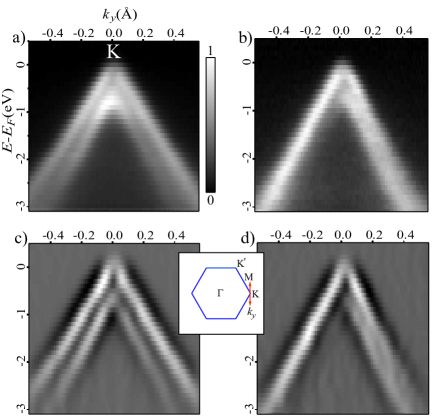
Figure 4: (Color online) Dispersion along the vertical ($k_{y}$) direction through the K̄ point for graphite obtained at photon energies of (a) $\hbar\omega=86$ eV and (b) $\hbar\omega=76$ eV. (c-d) Smoothed second derivative images of spectra shown in (a) and (b), respectively. Inset shows graphite surface Brillouin zone. Solid red line indicates $k_{y}$ direction through K̄ point.

For comparison with results on a known photoemission materials system, graphite spectra were taken at two photon energies (86 and 76 eV) along the same (vertical) direction through the K point; these results are shown in Fig. 4. The dispersion obtained at $\hbar\omega$=86 eV is clearly symmetric about the K point. At this photon energy we can resolve the splitting of the $\pi$ state into bonding and antibonding bands, with the two bands separated by $\sim$ 0.12 $\text{\AA}^{-1}$. The bands themselves are approximately 0.1 $\text{\AA}^{-1}$ in width. In the spectrum taken at 76 eV the two peaks are nearly degenerate. Again, the second derivative allows for easier determination of peak locations.

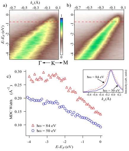
Figure 5: (Color online) ARPES intensity along $\Gamma$K direction in suspended monolayer graphene. Graphene photoemission taken with photon energies of (a) $\hbar\omega=50eV$ and (b) $\hbar\omega=84eV$. (c) HWHM of MDCs as a function of binding energy taken from (a) and (b). Inset shows sample MDCs taken 0.7 eV below $E_{F}$ as indicated by dashed red lines in (a) and (b).

Figure 5 shows the graphene dispersion taken along the $\Gamma$K direction through the K point. Comparative measurements were made at two different photon energies ($\hbar\omega=50,\hbar\omega=84$) and are shown in Fig. 5(a) and (b), respectively. In this direction, only one branch of the dispersion can be seen as the difference in phase between electron waves emitted from the A and B sub-lattice sites results in complete destructive interference. Shirley et al. (1995) Thus, this is a convenient direction along which to measure precisely the dispersion in the vicinity of the Dirac cone. The inset to Figure 5(c) compares momentum distribution curves (MDCs) taken at a binding energy of 0.7 eV for the suspended-graphene spectra at both photon energies. The data in Fig. 5(c) show that the width of the $\hbar\omega$=84 eV MDC is significantly larger than the $\hbar\omega$=50 eV MDC (0.17 $\text{\AA}^{-1}$ vs 0.12 $\text{\AA}^{-1}$).

Additionally, there is a slight asymmetry in all three MDCs as additional spectral weight is present on the right side of the peak (at higher values of $k_{x}$). The background signal decreases and the peaks become narrower for 50 eV photons as compared to 84 eV photons. Specifically, in the 0-4 eV range (referenced to $E_{F}$), the MDC width increases monotonically from 0.1 to 0.2 $\text{\AA}^{-1}$ and from 0.15 to 0.3 $\text{\AA}^{-1}$ for data collected with 50 eV photons and 84 eV photons, respectively. In contrast, MDCs taken along the same direction ($\Gamma$K) on supported graphene are significantly broaderKnox et al. (2008) and show almost no dependence on binding energy; they are $\sim$0.5 $\text{\AA}^{-1}$ in width from the Fermi energy to -4 eV binding energy. Thus, spectral features are sharpest for suspended samples measured with lower photon energy.

IV Discussion

IV.1 Comparison of Graphite and Graphene Results

As shown in Fig. 5, variation in photon energy results in changes to the linewidth of the graphene photoemission spectra, which can be exploited to sharpen the spectrum. In explaining these results on graphene, it is useful first to examine the effect of photon energy variation for the case of graphite. The differences in the measured photemission spectra of graphite taken at $\hbar\omega$=76 eV and $\hbar\omega$=86 eV shown in Figs. 4(a) and (b), respectively, are easily understood by considering the 3 dimensional band structure of graphite. In particular, according to the standard model of photoemission, variation in $\hbar\omega$ allows one to access a range of initial states with different $k_{z}$.Hüfner (2003) Using the free-electron approximation for the final state allows calculation of $k_{z}$ of the initial state.Hüfner (2003); Law et al. (1986) Thus, in the case of the data shown in Fig. 4, photoemission obtained at $\hbar\omega$ = 86 eV corresponds to $k_{z}$ = 0 (the $\Gamma$KM plane), while $\hbar\omega$ = 76 eV accesses $k_{z}$ = 0.3$c^{\ast}$ which is nearer the AHL plane. Since $k_{z}$ is changed, the clear double band feature seen for $k_{z}=0$ changes as the graphite band structure varies along $k_{z}$ in accord with the known graphite band structure. Shirley et al. (1995); Zhou et al. (2006); Sugawara et al. (2007); Law et al. (1986)

Consider now the effect of changing photon energies for the case of graphene photoemission. Since graphene is truly a 2D crystal, the initial states in the valence band are highly localized along the $z$ direction. Thus, the Brillouin zone is strictly 2 dimensional and the electronic strucure is essentially $k_{z}$ independent. Comparison with photoemission from surface states is useful, since they are also localized in 2D.Kevan and Gaylord (1987) However, the role of evanescent decay into the bulk, which is important for surface states in metals and results in a partial $k_{z}$ dependence,Kevan and Gaylord (1987) such as surface resonance, is absent in graphene and, thus, we may treat the initial state as independent of photon energy. In fact, as seen in Fig. 5, changing the photon energy in the case of graphene causes only a change in the overall linewidth and does not affect the measured bandstructure. As will be discussed below, the difference in the width of ARPES features between spectra obtained at $\hbar\omega$ =50 and $\hbar\omega$ =84 is a consequence of the surface roughness of the graphene samples. Since electrons in graphene propagate on a locally curved surface, the usual momentum conservation rules in ARPES must be modified and a photon-energy-dependent broadening term is introduced.

IV.2 General Considerations

In standard many-body ARPES theory, the intensity of the photoemission signal is proportional to the spectral function, $A({\bf k},\omega)$:

$$A({\bf k},\omega)=\frac{\text{Im}[\Sigma({\bf k},\omega)]}{(\omega-\omega_{\bf k}-\text{Re}[\Sigma({\bf k},\omega)])^{2}+\text{Im}[(\Sigma({\bf k},\omega)]^{2}}$$ (1)

where $\omega=E-E_{F}$ and ${\bf k}$ are binding energy and momentum, respectively, and $\omega_{\bf k}$ is the single-particle dispersion. The real and imaginary parts of the self-energy, $\Sigma({\bf k},\omega)$, represent renormalization of the bare-bands and scattering rate, respectively. To obtain the full expression for the photocurrent, the above function is then multiplied by energy and momentum-preserving delta functions, $\delta({\bf k}_{i}-{\bf k}_{f}-{\bf G})\delta(E_{i}-E_{f}-W)$, where $\bf G$ is a reciprocal lattice vector and i and f label the initial and final states, respectively, and $W$ is the work function of the material.

However, one major complication to this approach arises for the case of suspended graphene since the momentum preserving function, $\delta({\bf k}_{i}-{\bf k}_{f}-{\bf G})$, is only a precise delta-function if the system under investigation is atomically flat. While this is the case for the majority of single-crystal samples probed with ARPES, including the Kish graphite described above, exfoliated monolayer graphene, as is discussed in the Introduction, has significant deviations from planarity, ranging from 1 to 10 Å.Meyer et al. (2007) This corrugation introduces an additional broadening mechanism into the ARPES spectrum, which can be as large as, or larger than, the intrinsic broadening represented by $\text{Im}[\Sigma({\bf k},\omega)]$. Thus, in order to extract the true self-energy of carriers in the crystal, such corrugation-induced broadening must be taken into account. The MDCs are best fit by a convolution of $A({\bf k},\omega)$ with a function that represents broadening due to surface roughness. Thus, as will be shown below, at fixed $\omega$, photoemission intensity as a function of ${\bf k}_{\|}$ can be expressed as:

$$I({\bf k}_{\|})\propto\int d^{2}{\text{k}_{\|}}^{\prime}S_{k_{\perp}}({\bf k}_{\|})A({\bf k}_{\|}-{\bf k}^{\prime}_{\|},\omega)$$ (2)

where ${\bf k}_{\|}={\bf k}_{i\|}-{\bf k}_{f\|}$ and $S_{{\bf k}_{\perp}}$ represents corrugation-induced broadening. $S_{{\bf k}_{\perp}}$, the surface structure factor, is a function of the surface geometry of the sample and is also generally dependent on the change in perpendicular momentum from initial to final state, $k_{\perp}=k_{i\perp}-k_{f\perp}$. We note that several prior studies have examined the effect of surface roughness on ARPES measurements.Theilmann et al. (1999, 1997) In these prior studies, the roughness considered was due to discrete height variations caused by monatomic steps, rather than the continuous undulations of a thin film. Thus, the broadening in spectral features measured by ARPES was attributed to increased electron scattering rather than a variation in the phase of photoemitted electrons induced by local height fluctuations. In our experiments on suspended graphene samples, the surface morphology is carefully measured simultaneously with the ARPES measurements presented here, thus allowing us to determine $S_{{\bf k}_{\perp}}$ independently.Locatelli et al. (2006)

Finally, note that the surface corrugation of the graphene sheets will also alter the bandstructure by inducing a change in the local potential proportional to the square of the curvature. Thus, the ripples act as scattering centers, which will decrease lifetime and potentially change the Fermi velocity. These effects are contained in $A({\bf k},\omega)$ and will also be present in the ARPES data. However, such effects are distinct from that described by $S_{k_{\perp}}$, which represents decoherence as electrons pass from a curved 2D space to free space.

IV.3 Corrugation Broadening

Corrugation broadening can be treated by considering the equation that describes photoemission from a Bloch state in the graphene sheet into a free-electron state above the crystal. Using the standard tight-binding approach to describe the initial state:

$$\psi_{\bf k}({\bf r})=\frac{1}{\sqrt{N}}\sum_{\bf R}e^{i{\bf k}\cdot{\bf R}}\sum_{j=A,B}C^{\bf k}_{j}\phi({\bf r}-{\bf R}-\tau_{j})$$ (3)

we obtain the following matrix element for excitation into a free electron final state:

$$M\propto({\bf k_{i}}\cdot\hat{\bf{\lambda}})\sum_{j=A,B}C^{\bf k_{i}}_{j}e^{-i{\bf k_{f}}\cdot\tau_{j}}\sum_{R}e^{i({\bf k_{i}}-{\bf k_{f}})\cdot{\bf R}}\tilde{\phi}({\bf k_{f}})$$ (4)

where ${\bf k_{i}}$ is the initial pseudo-momentum of a valence-band electron and ${\bf k_{f}}$ is the final-state momentum (for a full description and definitions of symbols see Appendix). Equation 3 describes an initial state with precise momentum at a fixed binding energy. For an atomically-flat crystalline 2D surface the position vectors can be expressed as ${\bf R}=n_{1}\textbf{a}_{1}+n_{2}\textbf{a}_{2}$, where the $n_{i}$ are integers and the $\textbf{a}_{i}$ primitive lattice vectors in the $xy$ plane. In this case, the sum over R in Eq. 3, $\sum e^{i({\bf k_{i}}-{\bf k_{f}})\cdot{\bf R}}$, is zero unless ${\bf k_{i\|}}-{\bf k_{f\|}}={\bf G}$, where ${\bf G}$ is a reciprocal lattice vector. This condition is, thus, a statement of the momentum conservation discussed above, $\delta({\bf k_{i}}-{\bf k_{f}}-{\bf G})$. If, however, $z$ is allowed to vary continuously as a function of position along the surface, so that ${\bf R}=n_{1}\textbf{a}_{1}+n_{2}\textbf{a}_{2}+\Delta x+\Delta y+z$, with $z$ no longer constant, the summation in Eq. 4 is not as readily calculated. Perfect phase cancellation away from reciprocal lattice vectors does not occur, resulting in non-zero photoemisison intensity when ${\bf k_{i\|}}-{\bf k_{f\|}}\neq{\bf G}$.

Summations such as the one in Eq. 4 are encountered in the theory of LEED on rough surfaces.Lu and Lagally (1982); Yang et al. (1992, 1993) In fact, in many respects the formal analysis of LEED results bears many similarities to that of ARPES. In a prior study using one-photon photoemission and high-resolution LEED applied simultaneously to surface states of Cu(100) and Cu(111), it was demonstrated experimentally that the photoemission linewidth and the width of the LEED-spot profile are correlated linearly.Theilmann et al. (1997) In particular, for LEED one measures the diffraction structure factor, $S(\bf{k})\propto|\sum e^{i\bf{k}\cdot{\bf R}}|^{2}$ where, as in the case of photoemission, $\bf{k}$ is the total momentum transfer, ${\bf k}={\bf k_{i}}-{\bf k_{f}}$, and the sum is over atomic positions, $\bf R$, on a surface. In addition, for ARPES transition probability is proportional to the square of the matrix element; thus, the same structure factor, $S({\bf k})$, is applicable. Thus, LEED theory can guide our analysis.

The structure factor, $S({\bf k})$, can be calculated with information about the average properties of the surface, described by three variables: horizontal correlation-length, $\xi$, RMS height variation, $w$, and a dimensionless parameter, $\alpha$, termed the “roughness exponent,” which describes surface roughness on length scales smaller than $\xi$.Yang et al. (1993) All three parameters can be extracted from real-space information about the surface by computing the height-height correlation function, which is used in a variety of thin film measurements, including those on graphene and other surfaces, and is defined as $H(r)=\langle|z(r_{0}+r)-z(r_{0})|^{2}\rangle$. As is shown in the appendix, $S({\bf k})=S(k_{\perp},{\bf k_{\|}})$ is intimately related to $H(r)$ as the Fourier transform of $e^{-\frac{1}{2}k_{\bot}H(r)}$. Thus, the average parameters that characterize a given rough surface ($w$, $\xi$, and $\alpha$) and determine the form of $H(r)$ also determine $S({k_{\perp}},{\bf k_{\|}})$. Hence, with these parameters, it is possible to compute the summation in Eq. 4. In fact, previously reported measurements using low-energy electron microscopy and low-energy electron diffraction have determined these parameters to be $\alpha=0.54\pm 0.02$, $w=1.99\pm 0.15$ Å, and $\xi=30\pm 0.3$ nm for the same suspended graphene samples used in this study.Locatelli et al. (2010) Although the functional form of $S({k_{\perp}},{\bf k_{\|}})$ is complex, the width of $S_{k_{\perp}}({\bf k_{\|}})$ (i.e. for $k_{\perp}$ fixed) in ${\bf k_{\|}}$ space has a simple dependence on $k_{\perp}$ and the parameters describing the surface roughness. In particular, the width, $\Gamma_{S}$ is proportional to $(k_{\bot}w)^{\nicefrac{{1}}{{\alpha}}}$/$\xi$, which explains the decrease in experimental linewidth with decreasing $k_{\bot}$ shown in Fig. 5. For fitting purposes it is useful to have the exact functional form of $S_{k_{\perp}}({\bf k_{\|}})$. Yang, et al. have shown that for $(wk_{\perp})^{2}\gg 1$ the form is purely diffusive and can be expressed as:Yang et al. (1993)

$$S_{k_{\perp}}({\bf k_{\|}})=(\xi/(wk_{\perp})^{\nicefrac{{1}}{{\alpha}}})F_{\alpha}({\bf k_{\|}}\xi/(wk_{\perp})^{\nicefrac{{1}}{{\alpha}}})$$

$$F_{\alpha}(Y)=\int XdXexp(-X^{2\alpha})J_{0}(XY)$$ (5)

IV.4 Intrinsic Broadening

It is straightforward to introduce intrinsic initial-state broadening into our ARPES description by replacing our initial state wavefunction, $\psi_{\bf k}$, with a sum over multiple momentum states, $\sum a_{\bf k}\psi_{\bf k}$, where the $a_{\bf k_{i}}$ are complex coefficients related to the spectral function by $|a_{\bf k_{i}}|^{2}=A({\bf k},\omega)$. Our transition matrix then becomes a sum, $M=\sum a_{\bf k}M^{\bf k}$, over multiple matrix elements weighted by the complex coefficients $a_{\bf k}$, where the $M^{{\bf k}}$ are the original transition matrix elements defined in Eq. 4. Again, using Fermi’s golden rule we find that the transition probability is proportional to the square of this sum.

$$I\propto|M|^{2}=|\sum_{k}a_{k}M^{\bf k}|^{2}=\sum_{\bf k}|a_{\bf k}|^{2}|M^{k}|^{2}+\sum_{{\bf k}\neq{\bf k}^{\prime}}a_{\bf k}^{*}a_{\bf k^{\prime}}M^{{\bf k}*}M^{\bf k^{\prime}}$$ (6)

As shown in the appendix the ${\bf k}\neq{\bf k}^{\prime}$ sum can be safely neglected due to random phase cancellation and we arrive at the final expression for the full photoemission intensity expressed in Eq. 2.

Finally, we note that, in general, the linewidth ($\Gamma_{m}$) measured in ARPES from well prepared, atomically flat surfaces is a function of the initial state or photohole linewidth ($\Gamma_{i}$) as well as the linewidth of the final state or photoelectron ($\Gamma_{f}$). However, for the case of 2D states such as surface states in metals or thin films such as graphene, there is no dispersion with $k_{\perp}$ and $\Gamma_{m}=\Gamma_{i}$.Smith et al. (1993)

IV.5 Analysis of Spectra and Discussion

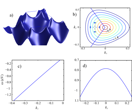
Figure 6: (Color online) (a) Graphene bandstructure over first BZ. (b) Contour lines drawn along constant binding energies in the vicinity of the K point (binding energies indicated in eV). (c-d) Dispersion along $k_{x}$ and $k_{y}$, respectively (along dashed blue lines in (b)).

Figure 3 shows a plot of the dispersion obtained along the $\Gamma$K direction in the vicinity of the Dirac point. The average Fermi velocity, derived from the slope of $\omega$ vs $k_{x}$ is $1.07\pm 0.05\times 10^{6}$ m/s. This value is in excellent agreement with results obtained by IR measurements on undoped supported exfoliated graphene.Jiang et al. (2007); Li et al. (2008) Additionally, the dispersion along $\Gamma$K is linear with no deviations from linearity within our experimental uncertainty. As discussed above, despite the roughness induced broadening in the spectrum, the dispersion curve is easily extracted from the raw ARPES data by taking the second derivative of the ARPES intensity along the momentum direction. However, determining the intrinsic width of spectral features requires a deeper analysis.

Our prior measurements of the surface corrugation in suspended graphene allow us to extract the intrinsic electronic structure from our ARPES data. The procedure for this fitting is as follows: first, $S_{k_{\perp}}$ is determined from our surface morphology measurements and used as a constant parameter, then $A({\bf k_{\|})}$ is varied until the convolved function, $I({\bf k_{\|}})$, represents a good fit to the experimental data. Although a full deconvolution is, in principle, possible it is much more straightforward to begin with an assumption for the functional form of $A({\bf k_{\|})}$ and systematically vary the parameters until a good fit is found. The functional form of $A({\bf k_{\|})}$ is assumed to be a Lorentzian, the most commonly used photoemission lineshape, which results from the $\bf k$-independent approximation for $\text{Im}[\Sigma({\bf k},\omega)]$.

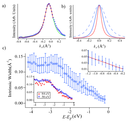
Figure 7: (Color online) Intrinsic width of ARPES features for Suspended monolayer graphene. (a) Example of MDC fitting. (b) Two independent contributions to broadening. Red line: intrinsic linewidth of initial state. Blue line: broadening due to corrugation at $\hbar\omega$=50 eV (solid) and $\hbar\omega$=84 eV (dashed). (c) Inverse lifetime as a function of binding energy for $\hbar\omega$=50 (blue) and $\hbar\omega$=84 eV (red). Inset shows best fit line to intrinsic width vs. binding energy for $\hbar\omega$=50 data in vicinity of Fermi level.

In carrying out this procedure, we introduce two additional simplifications. First, note that we are examining the region in $\bf k$-space within the first Brillouin zone along the $\Gamma$K ($k_{x}$) direction in the vicinity of the K point. As shown in Fig. 6, the $\pi$ state disperses rapidly along $k_{x}$ in this region, but relatively slowly along $k_{y}$ since $\partial\omega/\partial k_{y}$=0 at $k_{y}$=0. Thus, although Eq. 6 describes a 2D convolution, it is possible to replace the required 2D $k_{x}k_{y}$ integral with a 1D integral along $k_{x}$. Second, we note that most of the MDCs considered here have an asymmetric peak shape, with additional spectral weight in the $\omega>v_{F}|{\bf k}|$ region of the curve. Possible reasons for this asymmetry are discussed in a separate paragraph below. For fitting purposes, this additional spectral weight was not considered and the best fit was obtained by imposing a momentum cutoff within 0.1 $\text{\AA}^{-1}$ of the peak position on the $\omega>v_{F}|{\bf k}|$ side of the curve. Figure 7(a) shows a representative curve from the $\hbar\omega$=50 eV data taken 0.7 eV below the Fermi level along with a best fit. Note that the lineshape of this curve provides an excellent fit to the experimental data. Figure 7(b) shows the two independent contributions to the linewidth: the corrugation-induced broadening and the intrinsic broadening. In order to cross-check that the convolution procedure accurately captures the photon-energy dependence of the photoemission process, the same fitting procedure was repeated on data obtained with a photon energy of $\hbar\omega$=84. At this photon energy, $k_{\bot}=4.27\text{\AA}^{-1}$ and, according to Eq. 6, the width of $S_{k_{\perp}}$ is nearly twice as large as it is at $\hbar\omega=50$ eV. However, as expected, the intrinsic linewidth extracted from the fitting procedure is the same for data obtained with both photon energies. A comparison of the self-energy extracted from the two data sets is shown in Fig. 7(c); the two resulting curves are the same, within experimental error, thus confirming the photon-energy dependence given in Eq. 6 and lending further support to our approach.

To make our observations quantitative and enable comparison with other work, we perform a linear fit of the intrinsic width versus binding energy, $\Gamma_{i}=\alpha+\beta(E-E_{F})$. From this fit, we find $\alpha=0.002\pm 0.005$ $\text{\AA}^{-1}$ and $\beta=0.039\pm 0.01$ $\text{\AA}^{-1}eV^{-1}$. As expected, the value of $\alpha$ is within experimental uncertainty of zero since excited states just above the Fermi level should be very long lived. Consider now the parameter $\beta$ that describes the increase in inverse quasiparticle lifetime with increasing binding energy. The lifetime is related to $\Gamma_{i}$ by $\tau=1/(2\Gamma_{i}v_{F})$. Thus, our measured value can be reexpressed as $\beta$= 0.78$\pm$0.02 fs^-1 eV^-1, so as to enable ready comparison with prior measurements of the same quantity on graphite and exfoliated graphene. For graphite, $\beta$ has been measured by femtosecond photoemission to be an order of magnitude smaller, viz. 0.029 fs^-1 eV^-1,Xu et al. (1996) while STS measurements of exfoliated graphene on graphite have produced an intermediate value of ($\beta$ = 0.11 fs^-1 eV^-1).Li et al. (2009) A reasonable explanation for this discrepancy is the greater out-of-plane corrugation of suspended graphene, which has been predicted to be the largest contribution to electron scattering in rough graphene sheetsGazit (2009); Mariani and Von Oppen (2008); Katsnelson and Geim (2008). Indeed, such roughness constitutes short-range correlated disorder, which has also been shown theoretically to lead to scattering rates which scale linearly with $\omega$ in graphene.Foster and Aleiner (2008)

Comparison can also be made with results obtained on epitaxial graphene grown on SiC. In such a system the Dirac point is $\sim$ 0.5 eV below the Fermi level which changes the quasiparticle dynamics resulting in a non-linear behavior for $\Gamma_{i}$ vs $\omega$. In particular, it has been shown that electron-plasmon interaction in doped epitaxial graphene results in an increase in the electron scattering rate in a narrow energy region where $\omega\sim E_{D}$.Bostwick et al. (2006) However, at deeper binding energies a nearly linear increase of $\Gamma_{i}$ has been demonstrated with a slope of $\sim$ 0.025 $\text{\AA}^{-1}eV^{-1}$, which is comparable to our measured value of $\beta$.

Because of the unique Dirac Fermion behavior and two-dimensionality of graphene, there has been much discussion of many-body physics that would lead to lifetime broadening in ARPES measurements of grapheneBostwick et al. (2006); Das Sarma et al. (2007); Gonzalez et al. (1996, 2001). In conventional bulk crystals Fermi-liquid theory predicts the decay of a photohole through creation of an electron-hole pair to result in a lifetime which scales as $(E-E_{F})^{2}$, in proportion to the number of excitation pathways that satisfy momentum and energy conservation. However, the linear dispersion of the graphene bands along with the vanishing density of states at $E_{F}$ modify this picture. Hence, undoped graphene is expected to show anomalous marginal Fermi-liquid behavior, characterized by a lifetime that scales as $(E-E_{F})^{-1}$.Das Sarma et al. (2007) Electron-phonon interaction has also been shown experimentally to lead to linewidth broadening.Li et al. (2008); Bostwick et al. (2006) However, the interaction is limited by the phonon dispersion to within 140 meV of $E_{F}$.Liu et al. (2010) Coulombic interactions, however can affect scattering rates for electrons well below $E_{F}$. As noted above, elastic scattering due to short range correlated impurities such as adatoms, dislocations or corrugations has also been shown theoretically to produce a $(E-E_{F})^{-1}$ dependence on lifetime.Foster and Aleiner (2008)

As discussed above, prior STS measurements have confirmed this linear increase for a small range of energies ($\sim$150 meV) in the vicinity of the Fermi level for exfoliated graphene on graphite.Li et al. (2009) Our measurement confirms that this behavior persists as far as 2eV below the Fermi level; a log-log plot of $\Gamma_{i}$ vs $\omega$ displays a slope of $\sim$1. As noted above, such marginal Fermi-liquid behavior has also been observed by femtosecond time-resolved photoemission spectroscopy on graphite.Xu et al. (1996)

We now return to the topic of asymmetry in MDC peak shape. As many recent theoretical studies have pointed out, the commonly made $\bf k$-independent approximation for $\text{Im}[\Sigma({\bf k},\omega)]$ is not fully valid in graphene as the doping level approaches zero.Das Sarma et al. (2007); Gonzalez et al. (1996) The vanishing density of states at $\omega=E_{F}$ along with graphene’s linear dispersion near $E_{F}$ places a kinematic restriction on the available phase space for electron-electron scattering. The scattering pathway $e^{-}\rightarrow e^{-}+e^{-}h^{+}$ is only available for off-shell electrons for which $\omega>v_{F}|{\bf k}|$ and is kinematically forbidden when $\omega<v_{F}|{\bf k}|$. Thus, one expects a discontinuity in $\text{Im}[\Sigma({\bf k},\omega)]$ at $\omega=k$ and decay due to electron-electron interaction may be indicated by asymmetry in MDC peak shape.Foster and Aleiner (2008); Gonzalez et al. (1996) As mentioned above and indicated in Fig. 7, in MDCs taken through the K point for monolayer graphene additional spectral weight is present in the $\omega>v_{F}|{\bf k}|$ regime. In principle, a full deconvolution of the ARPES intensity would recover the exact function form of $A({\bf k},\omega)$. However, such a procedure would require use of the full 2D integral specified by Eq. 2, which is beyond the scope of the work presented here.

V Summary

Photoemission on thin sheets of 2D crystals is expected to grow in importance as interest in single layer insulators and semiconductors increases. We have performed ARPES on a 2D suspended surface with well defined surface corrugation. By comparing our work with our prior results obtained from diffraction measurements on corrugation in suspended graphene sheetsKnox et al. (2008) we have developed a model for understanding the effect of corrugation on ARPES spectra. By analyzing results obtained with different photon excitation energies, we have estimated the contribution of surface roughness to broadening. Thus, despite the surface corrugation in the graphene layer, it is still possible to develop insights into graphene physics. In particular, we have shown that exfoliated suspended graphene is essentially undoped in its pristine form. Additionally, we have shown that the band structure has no significant deviations from linearity in the vicinity of the Dirac point. Our measured Fermi velocity is comparable to results obtained on supported graphene by transport and optical measurements. Finally, we have also shown that undoped exfoliated graphene behaves as a marginal Fermi-liquid with an anomolous carrier lifetime, which scales as $(E-E_{F})^{-1}$.

*

Appendix A

In this appendix, we will follow the standard formalism for single photon photoemission using the dipole approximation. We will adapt the treatment to deal with a locally curved surface using a specific initial state described by the tight binding model for graphene.

According to the standard tight-binding scheme, initial $\pi$ states in the valence band of graphene with energy $\omega_{k}$ and crystal-momentum ${\bf k}$ are represented as a linear combination of molecular $p_{z}$ orbital states:

$$\psi_{\bf k}({\bf r})=\frac{1}{\sqrt{N}}\sum_{\bf R}e^{i{\bf k}\cdot{\bf R}}\sum_{j=A,B}C^{\bf k}_{j}\phi({\bf r}-{\bf R}-\tau_{j})$$ (7)

where $\frac{1}{\sqrt{N}}$ is an overall normalization factor, $A$ and $B$ designate the sublattice sites and $\tau_{j}$ their locations within the unit cell. The $C^{\bf k}_{j}$ are complex coefficients obtained from the tight-binding model and the $\phi$ are molecular $p_{z}$ orbitals. The sum over ${\bf R}$ runs over all $N$ unit cells in the crystal (note that we work in the limit where $N\rightarrow\infty$).

The transition-matrix for photoexcitation from this initial state to a plane wave final state with total momentum $\bf{k}_{f}$ outside the crystal can be written, using the dipole approximation, as follows:

$$M^{\bf{k}}\propto\int d^{3}re^{-i{\bf k}_{f}\cdot{\bf r}}({\bf p}\cdot{\bf A})\psi_{\bf{k}_{i}}({\bf r})$$ (8)

Inserting the above definition for the initial state we obtain:

$$M^{\bf{k}}\propto({\bf k_{i}}\cdot\hat{\bf{\lambda}})\sum_{R}e^{i({\bf k_{i}}-{\bf k_{f}})\cdot{\bf R}}\tilde{\phi}(k_{f})\sum_{j=A,B}C^{\bf k}_{j}e^{-i{\bf k_{f}}\cdot\tau_{j}}$$ (9)

where $\tilde{\phi}$ is the Fourier transform of the molecular $p_{z}$ orbital and $\hat{\bf{\lambda}}$ represents the polarization vector of the incoming radiation. We are interested in a small region of momentum-space in the vicinity of the K point. Since ${\bf k_{i}}\cdot\hat{{\bf\lambda}}$ and $\tilde{\phi}({\bf k_{f}})$ are nearly constant in this region, we concentrate our attention on the sum, $\sum e^{i({\bf k_{i}}-{\bf k_{f}})\cdot{\bf R}}\sum C^{\bf k_{i}}_{j}e^{-i{\bf k_{i}}\cdot\tau_{j}}$. The sum over $j$, $\sum C^{\bf k_{i}}_{j}e^{-i{\bf k_{f}}\cdot\tau_{j}}$, depends only on the relative phase between the $C^{\bf k}_{j}$’s and the pathlength difference from atoms $A$ and $B$ to the detector. This term changes rapidly on a contour around the K point. Along the $\Gamma$K direction, the term changes from 2 to 0 as we pass through the K point from the first to the second BZ. However, if we restrict ourselves to the region of ${\bf k}$-space along the $\Gamma$K direction within the first BZ (see Fig 6), $\sum C^{\bf k_{i}}_{j}e^{-i{\bf k_{f}}\cdot\tau_{j}}$ is nearly constant. Thus, we are left with the sum $\sum e^{i({\bf k_{i}}-{\bf k_{f}})\cdot{\bf R}}$.

For a 3D crystal with perfect translational symmetry ${\bf R}=n_{1}{\bf a_{1}}+n_{2}{\bf a_{2}}+n_{3}{\bf a_{3}}$ where $n_{1},n_{2},n_{3}$ are integers and ${\bf a_{1}},{\bf a_{2}},{\bf a_{3}}$ are primitive lattice vectors. In this case, the sum over ${\bf R}$ reduces to momentum preserving delta function $\delta({\bf k_{f}}-{\bf k_{i}}-{\bf G})$ where $G$ is a reciprocal lattice vector. However, since graphene is a two-dimensional lattice, momentum conservation does not hold in the perpendicular direction. More significantly, exfoliated graphene is a flexible membrane that is not atomically flat, so the R’s must be expressed in terms of a continuous variable; thus ${\bf R}=n_{1}\textbf{a}_{1}+n_{2}\textbf{a}_{2}+\Delta x+\Delta y+z$, where $z_{j}$ is a continuous variable which represents the local height of the graphene sheet. The variation in height is such that we can consider the well known theory of scattering from continuous rough surfaces in order to evaluate the sum in equation 9. We begin by replacing the discrete sum with an integral:

$$\sum_{\bf R}e^{i({\bf k_{i}}-{\bf k_{f}})\cdot{\bf R}}=\int d^{3}rD({\bf r})e^{i({\bf k_{i}}-{\bf k_{f}})\cdot{\bf r}}$$ (10)

where $D(r)$ is the density-function of the material which, for a perfectly crystalline flat sample, has the form:

$$D({\bf r})=\sum_{\bf R}\delta({\bf r}-{\bf R})$$ (11)

A periodic lattice generates a photoemission spectrum with the periodicity of the reciprocal lattice. However, since we are concerned with the photoemission spectrum in a small region of $\bf k$-space in the first Brillouin zone, we may abandon the description of the surface as a discrete lattice and replace it with a smooth, continuous sheet. Thus, we approximate $D(r)$ as a surface density function:

$$D({\bf\rho},z^{\prime})\simeq\delta[z^{\prime}-z({\bf\rho})]$$ (12)

where $\mathbf{\rho}=r_{\|}=(x,y)$ and $z^{\prime}=r_{\perp}$. Thus, the surface is now defined by the height function $z=z(\mathbf{\rho})$. Inserting the above definition of $D(r)$ and explicitly separating $\bf k_{i}$ and $\bf k_{f}$ into components parallel and perpendicular to the surface we obtain:

$$M\propto\int d^{2}\rho e^{i({\bf k_{i}}_{\perp}-{\bf k_{f}}_{\perp})\cdot z(\rho)}e^{i({\bf k_{i}}_{\|}-{\bf k_{f}}_{\|})\cdot\rho}$$ (13)

We have retained momentum conservation; for a constant $z(\rho)$ the above integral produces $\delta({\bf k_{i}}_{\|}-{\bf k_{f}}_{\|})$ times a complex phase; but for a non-trivial $z(\rho)$, the delta function broadens since $e^{i({\bf k_{i}}_{\perp}-{\bf k_{f}}_{\perp})\cdot z(\rho)}$ is no longer independent of $\rho$. Additionally, electronic states in graphene propagate on a curved space, which implies that the direction of the initial state wavevector, ${\bf k_{i}}$, varies as a function of position along the surface so that $k_{i\perp}$ and $k_{i\|}$ vary with $\rho$ as well. This introduces additional phase variation into the exponential argument $({\bf k_{i}}_{\perp}-{\bf k_{f}}_{\perp})\cdot z(\rho)$. However, this variation is very small in comparison to that introduced by changes in $z(\rho)$ and can effectively be ignored with little change in our final result. In particular, $k_{i\perp}$ varies proportional to $k\frac{\partial z}{\partial\rho_{k}}$ which is on the order of 0.01 Å^-1. Thus the phase variation in the term $k_{i\perp}z\ll 1$ ($\Delta z\approx$ 2 Å) is very small in comparison to the variation in the $k_{f\perp}z$ term ($k_{f\perp}$ ranges from 2.5 to 3.5 Å^-1). Thus, we will approximate the direction of the initial state wavevector, ${\bf k_{i}}$, as constant for all points on the surface. This means that $\bf k$ is not $\rho$ dependent and we can define a new vector ${\bf k}={\bf k_{i}}-{\bf k_{f}}$, so that our expression becomes:

$$M\propto\int d^{2}\rho e^{i{\bf k}_{\perp}\cdot z(\rho)}e^{i{\bf k}_{\|}\cdot\rho}$$ (14)

To find the photoemission intensity we use Fermi’s golden rule which yields:

$$I\propto\frac{2\pi}{\hbar}\|M\|^{2}$$

$$\|M\|^{2}\propto\int d^{2}\rho^{\prime}d^{2}\rho e^{i{\bf k}_{\perp}\cdot z(\rho)}$$

$$\times e^{i{\bf k}_{\|}\cdot\rho}e^{-i{\bf k}_{\perp}\cdot z(\rho^{\prime})}e^{-i{\bf k}_{\|}\cdot\rho^{\prime}}$$ (15a)

Defining $r=\rho-\rho^{\prime}$ we can rearrange to obtain:

$$I\propto\int d^{2}r\left(\int d^{2}\rho e^{i{\bf k}_{\perp}\cdot[z(\rho+r)-z(\rho)]}\right)e^{i{\bf k}_{\|}\cdot r}$$ (16)

The term inside the parenthes is the height-difference function, $C(r,k_{\perp})$, of the surface which is related to the height-height correlation function, $H(r)=\langle|z(r_{0}+r)-z(r_{0})|^{2}\rangle$. It is straight forward to show that the $C(r,k_{\perp})$ equals $e^{-\frac{1}{2}H(r)k_{\perp}^{2}}$.Yang et al. (1993) Thus, we have:

$$I\propto\int d^{2}rC(k_{\perp},r)e^{i{\bf k}_{\|}\cdot r},$$ (17a)

$$C(k_{\perp},r)=e^{-\frac{1}{2}H(r)k_{\perp}^{2}}.$$ (17b)

For a large class of surfaces, $H(r)$ has the following properties:

$$H(r)\propto e^{2\alpha},\text{for }r\ll\xi$$ (18)

$$H(r)=2w^{2},\text{for }r\gg\xi$$ (19)

where $\alpha$ is a measure of the small scale roughness termed the “roughness exponent.” In, particular, it can be shown that the full width at half maximum (FWHM) of $I(k_{\|})$ (with $k_{\perp}$ held constant) scales as $\xi^{-1}(wk_{\perp})^{\frac{1}{\alpha}}$ when $(wk_{\perp})^{2}\gg 1$. The functional form of $I(k_{\|})$ is well approximated as:Yang et al. (1993)

$$S_{k_{\perp}}({\bf k_{\|}})=(\xi/(wk_{\perp})^{\nicefrac{{1}}{{\alpha}}})F_{\alpha}({\bf k_{\|}}\xi/(wk_{\perp})^{\nicefrac{{1}}{{\alpha}}})$$

$$F_{\alpha}(Y)=\int XdXexp(-X^{2\alpha})J_{0}(XY)$$ (20)

The above discussion began with the assumption that the initial state, $\psi_{k}$, had a well defined pseudo-momentum, $k$, and energy $\omega_{k}$. To include initial state broadening in our description, we replace $\psi_{k}$ with a sum over multiple momentum states, $\sum a_{k}\psi_{k}$, where the $a_{k}$ are complex coefficients. The coefficients, $a_{k}$, are related to the spectral function, $A(k,\omega)$ by $|a_{k}|^{2}=A(k,\omega)$ with the spectral function defined as:

$$A(k,\omega)=\frac{Im(\Sigma)}{(\omega_{k}-\omega-Re(\Sigma))^{2}+Im(\Sigma)^{2}}$$ (21)

where $\Sigma=\Sigma(k,\omega)$ is the quasiparticle self-energy. Retaining our simple description of the final state as a free-electron state with momentum $q$, our transition matrix becomes a sum, $M=\sum a_{k}M^{kq}$, over multiple matrix elements weighted by the complex coefficients $a_{k}$, where the $M^{kq}$ are the original transition matrix elements defined in Eq. 9. Again, using Fermi’s golden rule we find that the transition probability is proportional to the square of this sum:

$$I\propto|M|^{2}=|\sum_{k}a_{k}M^{kq}|^{2}=$$

$$\sum_{k}|a_{k}|^{2}|M^{kq}|^{2}+\sum_{k\neq k^{\prime}}a_{k}^{*}a_{k^{\prime}}M^{kq*}M^{k^{\prime}q}$$ (22)

The cross terms have the form:

$$M^{kq*}M^{k^{\prime}q}\propto\int d^{2}r\left(\int d^{2}\rho e^{i{\bf k}_{\perp}\cdot[z(\rho+r)-z(\rho)]}e^{i\Delta{\bf k}_{\|}\rho}\right)e^{i{\bf k^{\prime}}_{\|}\cdot r}$$ (23)

where $\Delta{\bf k}_{\|}={\bf k^{\prime}}_{\|}-{\bf k}_{\|}$, ${\bf k}_{\perp}\approx{\bf k^{\prime}}_{\perp}$. The $e^{i\Delta{\bf k}_{\|}\rho}$ factor in the $\rho$ integral introduces a random phase that causes the integral to average to zero (since it is taken over the whole surface). Thus, the cross terms can be safely neglected and we arrive at the final expression or photoemission intensity as a function of $k_{\|}$ with $k_{\perp}$ fixed, described by Eq. 2.

References

- Novoselov et al. (2005) K. Novoselov, A. Geim, S. Morozov, D. Jiang, M. Grigorieva, S. Dubonos, and A. Firsov, Nature 438, 197 (2005).
- Zhang et al. (2005) Y. Zhang, Y. Tan, H. Stormer, and P. Kim, Nature 438, 201 (2005).
- Neto et al. (2009) A. Neto, F. Guinea, N. Peres, K. Novoselov, and A. Geim, Reviews of Modern Physics 81, 109 (2009).
- Ohta et al. (2006) T. Ohta, A. Bostwick, T. Seyller, K. Horn, and E. Rotenberg, Science 313, 951 (2006).
- Bostwick et al. (2006) A. Bostwick, T. Ohta, T. Seyller, K. Horn, and E. Rotenberg, Nature Physics 3, 36 (2006).
- Dedkov et al. (2008) Y. Dedkov, M. Fonin, U. Rüdiger, and C. Laubschat, Physical Review Letters 100, 107602 (2008).
- Shikin et al. (2000) A. Shikin, G. Prudnikova, V. Adamchuk, F. Moresco, and K. Rieder, Physical Review B 62, 13202 (2000).
- Vázquez de Parga et al. (2008) A. Vázquez de Parga, F. Calleja, B. Borca, M. Passeggi Jr, J. Hinarejos, F. Guinea, and R. Miranda, Physical Review Letters 100, 56807 (2008).
- Liu et al. (2010) Y. Liu, L. Zhang, M. Brinkley, G. Bian, T. Miller, and T. Chiang, Physical Review Letters 105, 136804 (2010).
- Pletikosić et al. (2009) I. Pletikosić, M. Kralj, P. Pervan, R. Brako, J. Coraux, A. N Diaye, C. Busse, and T. Michely, Physical Review Letters 102, 56808 (2009).
- Sutter et al. (2009) P. Sutter, M. Hybertsen, J. Sadowski, and E. Sutter, Nano Letters 9, 2654 (2009).
- Valla et al. (2009) T. Valla, J. Camacho, Z. Pan, A. Fedorov, A. Walters, C. Howard, and M. Ellerby, Physical Review Letters 102, 107007 (2009).
- Sprinkle et al. (2009) M. Sprinkle, D. Siegel, Y. Hu, J. Hicks, A. Tejeda, A. Taleb-Ibrahimi, P. Le Fèvre, F. Bertran, S. Vizzini, H. Enriquez, et al., Physical Review Letters 103, 226803 (2009).
- Knox et al. (2008) K. Knox, S. Wang, A. Morgante, D. Cvetko, A. Locatelli, T. Mentes, M. Niño, P. Kim, and R. Osgood Jr, Physical Review B 78, 201408 (2008).
- Bolotin et al. (2008) K. Bolotin, K. Sikes, Z. Jiang, M. Klima, G. Fudenberg, J. Hone, P. Kim, and H. Stormer, Solid State Communications 146, 351 (2008).
- Wang et al. (2008) F. Wang, Y. Zhang, C. Tian, C. Girit, A. Zettl, M. Crommie, and Y. Shen, Science 320, 206 (2008).
- Mak et al. (2010) K. Mak, M. Sfeir, J. Misewich, and T. Heinz, Proceedings of the National Academy of Sciences 107, 14999 (2010).
- Fujikawa et al. (2009) Y. Fujikawa, T. Sakurai, and R. Tromp, Physical Review B 79, 121401 (2009).
- Geringer et al. (2009) V. Geringer, M. Liebmann, T. Echtermeyer, S. Runte, M. Schmidt, R. Ruckamp, M. Lemme, and M. Morgenstern, Physical Review Letters 102, 76102 (2009).
- Ishigami et al. (2007) M. Ishigami, J. Chen, W. Cullen, M. Fuhrer, and E. Williams, Nano Letters 7, 1643 (2007).
- Locatelli et al. (2010) A. Locatelli, K. Knox, D. Cvetko, T. Mentes, M. Niño, S. Wang, M. Yilmaz, P. Kim, R. Osgood Jr, and A. Morgante, ACS Nano 4, 4879 (2010).
- Stolyarova et al. (2007) E. Stolyarova, K. Rim, S. Ryu, J. Maultzsch, P. Kim, L. Brus, T. Heinz, M. Hybertsen, and G. Flynn, Proceedings of the National Academy of Sciences 104, 9209 (2007).
- Cullen et al. (2010) W. Cullen, M. Yamamoto, K. Burson, J. Chen, C. Jang, L. Li, M. Fuhrer, and E. Williams, Physical Review Letters 105, 215504 (2010).
- Locatelli et al. (2003) A. Locatelli, A. Bianco, D. Cocco, S. Cherifi, S. Heun, M. Marsi, M. Pasqualetto, and E. Bauer, J. Phys. IV France 104, 99 (2003).
- Schmidt et al. (1998) T. Schmidt, S. Heun, J. Slezak, J. Diaz, K. Prince, G. Lilienkamp, and E. Bauer, Surface Review and Letters 5, 1287 (1998).
- Locatelli and Bauer (2008) A. Locatelli and E. Bauer, Journal of Physics: Condensed Matter 20, 093002 (2008).
- Locatelli et al. (2006) A. Locatelli, L. Aballe, T. Mentes, M. Kiskinova, and E. Bauer, Surface and Interface Analysis 38, 1554 (2006).
- Hibino et al. (2008) H. Hibino, H. Kageshima, F. Maeda, M. Nagase, Y. Kobayashi, and H. Yamaguchi, Physical Review B 77, 75413 (2008).
- Altman (2005) M. Altman, Journal of Physics: Condensed Matter 17, S1305 (2005).
- Shirley et al. (1995) E. Shirley, L. Terminello, A. Santoni, and F. Himpsel, Physical Review B 51, 13614 (1995).
- Hüfner (2003) S. Hüfner, Photoelectron spectroscopy: principles and applications (Springer Verlag, 2003).
- Law et al. (1986) A. Law, M. Johnson, and H. Hughes, Physical Review B 34, 4289 (1986).
- Zhou et al. (2006) S. Zhou, G. Gweon, J. Graf, A. Fedorov, C. Spataru, R. Diehl, Y. Kopelevich, D. Lee, S. Louie, and A. Lanzara, Nature Physics 2, 595 (2006).
- Sugawara et al. (2007) K. Sugawara, T. Sato, S. Souma, T. Takahashi, and H. Suematsu, Physical Review Letters 98, 36801 (2007).
- Kevan and Gaylord (1987) S. Kevan and R. Gaylord, Physical Review B 36, 5809 (1987).
- Meyer et al. (2007) J. Meyer, A. Geim, M. Katsnelson, K. Novoselov, T. Booth, and S. Roth, Nature 446, 60 (2007).
- Theilmann et al. (1999) F. Theilmann, R. Matzdorf, and A. Goldmann, Surface science 420, 33 (1999).
- Theilmann et al. (1997) F. Theilmann, R. Matzdorf, G. Meister, and A. Goldmann, Physical Review B 56, 3632 (1997).
- Note (1) It is implied here that , and are functions of position along the surface with representing the local height of the surface and , representing deviations from the ideal lateral positions of surface atoms which are necessary to keep the average bond length unchanged.
- Lu and Lagally (1982) T. Lu and M. Lagally, Surface Science 120, 47 (1982).
- Yang et al. (1992) H. Yang, T. Lu, and G. Wang, Physical Review Letters 68, 2612 (1992).
- Yang et al. (1993) H. Yang, G. Wang, and T. Lu, Diffraction from rough surfaces and dynamic growth fronts (World Scientific Pub Co Inc, 1993).
- Smith et al. (1993) N. Smith, P. Thiry, and Y. Petroff, Physical Review B 47, 15476 (1993).
- Jiang et al. (2007) Z. Jiang, E. Henriksen, L. Tung, Y. Wang, M. Schwartz, M. Han, P. Kim, and H. Stormer, Physical Review Letters 98, 197403 (2007).
- Li et al. (2008) Z. Li, E. Henriksen, Z. Jiang, Z. Hao, M. Martin, P. Kim, H. Stormer, and D. Basov, Nature Physics 4, 532 (2008).
- Note (2) In fitting the MDCs an instrumental broadening term was also convolved with our spectral function. The energy resolution introduces a width of . In combination with the lateral resolution of the instrument (known from prior calibration), this results in a Gaussian response function with a width of approximately 0.042 .
- Xu et al. (1996) S. Xu, J. Cao, C. Miller, D. Mantell, R. Miller, and Y. Gao, Physical Review Letters 76, 483 (1996).
- Li et al. (2009) G. Li, A. Luican, and E. Andrei, Physical Review Letters 102, 176804 (2009).
- Gazit (2009) D. Gazit, Physical Review B 79, 113411 (2009).
- Mariani and Von Oppen (2008) E. Mariani and F. Von Oppen, Physical Review Letters 100, 76801 (2008).
- Katsnelson and Geim (2008) M. Katsnelson and A. Geim, Philosophical Transactions A 366, 195 (2008).
- Foster and Aleiner (2008) M. Foster and I. Aleiner, Physical Review B 77, 195413 (2008).
- Das Sarma et al. (2007) S. Das Sarma, E. Hwang, and W. Tse, Physical Review B 75, 121406 (2007).
- Gonzalez et al. (1996) J. Gonzalez, F. Guinea, and M. Vozmediano, Physical Review Letters 77, 3589 (1996).
- Gonzalez et al. (2001) J. Gonzalez, F. Guinea, and M. Vozmediano, Physical Review B 63, 134421 (2001).