Load-Balancing Spatially Located Computations using Rectangular Partitions

Abstract

Distributing spatially located heterogeneous workloads is an important problem in parallel scientific computing. We investigate the problem of partitioning such workloads (represented as a matrix of non-negative integers) into rectangles, such that the load of the most loaded rectangle (processor) is minimized. Since finding the optimal arbitrary rectangle-based partition is an NP-hard problem, we investigate particular classes of solutions: rectilinear, jagged and hierarchical. We present a new class of solutions called $m$-way jagged partitions, propose new optimal algorithms for $m$-way jagged partitions and hierarchical partitions, propose new heuristic algorithms, and provide worst case performance analyses for some existing and new heuristics. Moreover, the algorithms are tested in simulation on a wide set of instances. Results show that two of the algorithms we introduce lead to a much better load balance than the state-of-the-art algorithms. We also show how to design a two-phase algorithm that reaches different time/quality tradeoff.

Keywords: Load balancing; spatial partitioning; optimal algorithms; heuristics; dynamic programming; particle-in-cell; mesh-based computation; jagged partitioning; rectilinear partitioning; hierarchical partitioning

1 Introduction

To achieve good efficiency when using a parallel platform, one must distribute the computations and the required data to the processors of the parallel machine. If the computation tasks are independent, their parallel processing falls in the category of pleasantly parallel tasks. Even in such cases, when computation time of the tasks are not equal, obtaining the optimal load balance to achieve optimum execution time becomes computationally hard and heuristic solutions are used [22]. Furthermore, most of the time some dependencies exist between the tasks and some data must be shared or exchanged frequently, making the problem even more complicated.

A large class of application see its computations take place in a geometrical space of typically two or three dimensions. Different types of applications fall into that class. Particle-in-cell simulation [33, 17] is an implementation of the classical mean-field approximation of the many-body problem in physics. Typically, thousands to millions of particles are located in cells, which are a discretization of a field. The application iteratively updates the value of the field in a cell, based on the state of the particles it contains and the value of the neighboring cells, and then the state of the particles, based on its own state and the state of the cell it belongs to. Direct volume rendering [20] is an application that use rendering algorithm similar to raycasting in a scene of semi-transparent objects without reflection. For each pixel of the screen, a ray orthogonal to the screen is cast from the pixel and color information will be accumulated over the different objects the ray encounters. Each pixel therefore requires an amount of computation linear to the number of objects crossed by the ray and neighboring pixels are likely to cross the same objects. Partial Differential Equation can be computed using mesh-based computation. For instance [16] solves heat equation on a surface by building a regular mesh out of it. The state of each node of the mesh is iteratively updated depending on the state of neighboring nodes. For load balancing purpose, [27] maps the mesh to a discretized two dimensional space. An other application can be found in 3D engines where the state of the world is iteratively updated and where the updates on each object depends on neighboring objects (for instance, for collision purpose) [1]. Linear algebra operations can potentially also benefit from such techniques [37, 30, 36].

In this work, our goal is to balance the load of such applications. In the literature, load balancing techniques can be broadly divided into two categories: geometric and connectivity-based. Geometric methods (such as [5, 29]) leverages the fact that computations which are close by in the space are more likely to share data than computations that are far in the space, by dividing the load using geometric properties of the workload. Methods from that class often rely on a recursive decomposition of the domain such as octrees [9] or they rely on space filling curves and surfaces [2, 3]. Connectivity-based methods usually model the load balancing problem through a graph or an hypergraph weighted with computation volumes on the nodes and communication volumes on the edges or hyper edges (see for instance [35, 8]). Connectivity-based techniques lead to good partitions but are usually computationally expensive and require to build an accurate graph (or hypergraph) model of the computation. They are particularly well-suited when the interactions between tasks are irregular. Graphs are useful when modeling interactions that are exactly between two tasks, and hypergraph are useful when modeling more complex interactions that could involve more than two tasks [7, 15].

When the interactions are regular (structured) one can use methods that takes the structure into account. For example, when coordinate information for tasks are available, one can use geometric methods which leads to “fast” and effective partitioning techniques. In geometric partitioning, one prefers to partition the problem into connex and compact parts so as to minimize communication volumes. Rectangles (and rectangular volumes) are the most preferred shape because they implicitly minimize communication, do not restrict the set of possible allocations drastically, are easily expressed and allow to quickly find which rectangle a coordinate belongs to using simple data structures. Hence, in this work, we will only focus partitioning into rectangles.

In more concrete terms, this paper addresses the problem of partitioning a two-dimensional load matrix composed of non-negative numbers into a given number of rectangles (processors) so as to minimize the load of the most loaded rectangle; the most loaded rectangle is the one whose sum of the element it contains is maximal. The problem is formulated so that each element of the array represents a task and each rectangle represents a processor. Computing the optimal solution for this problem has been shown to be NP-Hard [13]. Therefore, we focus on algorithms with low polynomial complexity that lead to good solutions.

The approach we are pursuing in this work is to consider different classes of rectangular partitioning. Simpler structures are expected to yield bad load balance but to be computed quickly while more complex structures are expected to give good load balance but lead to higher computation time. For each class, we look for optimal algorithms and heuristics. Several algorithms to deal with this particular problem which have been proposed in the literature are described and analyzed. One original class of solution is proposed and original algorithms are presented and analyzed.

The theoretical analysis of the algorithms is accompanied by an extensive experimentation evaluation of the algorithms to decide which one should be used in practice. The experimentation is composed of various randomly generated datasets and two datasets extracted from two applications, one following the particle-in-cell paradigm and one following the mesh-based computation paradigm.

The contributions of this work are as follows:

• A classical $P\!\times\!Q$-way jagged heuristic is theoretically analyzed by bounding the load imbalance it generates in the worst case.

• We propose a new class of solutions, namely, $m$-way jagged partitions, for which we propose a fast heuristic as well as an exact polynomial dynamic programming formulation. This heuristic is also theoretically analyzed and shown to perform better than the $P\!\times\!Q$-way jagged heuristic.

• For an existing class of solutions, namely, hierarchical bipartitions, we propose both an optimal polynomial dynamic programming algorithm as well as a new heuristic.

• The presented and proposed algorithms are practically assessed in simulations performed on synthetic load matrices and on real load matrices extracted from both a particle-in-cell simulator and a geometric mesh. Simulations show that two of the proposed heuristics outperform all the tested existing algorithms.

• Algorithmic engineering techniques are used to create hybrid partitioning scheme that provides slower algorithms but with higher quality.

This work extends [34] by providing the following main contributions: tighter bounds in the theoretical guarantee of an $m$-way jagged partitioning heuristic, new heuristics for $m$-way jagged partitioning, experimental results of proposed algorithms with detailed charts, and hybrid algorithms.

Several previous work tackles a similar problem but they usually presents only algorithms from one class with no experimental validation or a very simple one. These works are referenced in the text when describing the algorithm they introduce. Kutluca et al. [20] is the closest related work. They are tackling the parallelization of a Direct Volume Rendering application whose load balancing is done using a very similar model. They survey rectangle based partition but also more general partition generated from hypergraph modeling and space filling curves. The experimental validation they propose is based on the actual runtime of the Direct Volume Rendering application.

Similar classes of solutions are used in the problem of partitioning an equally loaded tasks onto heterogeneous processors (see [21] for a survey). This is a very different problem which often assumes the task space is continuous (therefore infinitely divisible). Since the load balance is trivial to optimize in such a context, most work in this area focus on optimizing communication patterns.

The rest of the paper is organized as follows. Section 2 presents the model and notations used. The different classes of partitions are described in Section 3. This section also presents known and new polynomial time algorithms either optimal or heuristic. The algorithms are evaluated in Section 4 on synthetic dataset as well as on dataset extracted from two real simulation codes. Section 5 presents a two-phase technique, namely hybrid algorithms, to generate partitions. Conclusive remarks are given in Section 6.

2 Model and Preliminaries

2.1 Problem Definition

Let $A$ be a two dimensional array of $n_{1}\times n_{2}$ non-negative integers representing the spatially located load. This load matrix needs to be distributed on $m$ processors. Each element of the array must be allocated to exactly one processor. The load of a processor is the sum of the elements of the array it has been allocated. The cost of a solution is the load of the most loaded processor. The problem is to find a solution that minimizes the cost.

In this paper we are only interested in rectangular allocations, and we will use ’rectangle’ and ’processor’ interchangeably. That is to say, a solution is a set $R$ of $m$ rectangles $r_{i}=(x_{1},x_{2},y_{1},y_{2})$ which form a partition of the elements of the array. Two properties have to be ensured for a solution to be valid: $\bigcap_{r\in R}=\emptyset$ and $\bigcup_{r\in R}=A$. The first one can be checked by verifying that no rectangle collides with another one, it can be done using line to line tests and inclusion test. The second one can be checked by verifying that all the rectangles are inside $A$ and that the sum of their area is equal to the area of $A$. This testing method runs in $O(m^{2})$. The load of a processor is $L(r_{i})=\sum_{x_{1}\leq x\leq x_{2}}\sum_{y_{1}\leq y\leq y_{2}}A[x][y]$. The load of the most loaded processor in solution $R$ is $L_{max}=\max_{r_{i}}L(r_{i})$. We will denote by $L_{max}^{*}$ the minimal cost achievable. Notice that $L_{max}^{*}\geq\frac{\sum_{x,y}A[x][y]}{m}$ and $L_{max}^{*}\geq\max_{x,y}A[x][y]$ are lower bounds of the optimal maximum load. In term of distributed computing, it is important to remark that this model is only concerned by computation times and not by communication times.

Algorithms that tackle this problem rarely consider the load of a single element of the matrix. Instead, they usually consider the load of a rectangle. Therefore, we assume that matrix $A$ is given as a 2D prefix sum array $\Gamma$ so that $\Gamma[x][y]=\sum_{x^{\prime}\leq x,y^{\prime}\leq y}A[x^{\prime}][y^{\prime}]$. That way, the load of a rectangle $r=(x_{1},x_{2},y_{1},y_{2})$ can be computed in $O(1)$ (instead of $O((x_{2}-x_{1})(y_{2}-y_{1}))$), as $L(r)=\Gamma[x_{2}][y_{2}]-\Gamma[x_{1}-1][y_{2}]-\Gamma[x_{2}][y_{1}-1]+\Gamma[x_{1}-1][y_{1}-1]$.

An algorithm $H$ is said to be a $\rho$-approximation algorithm, if for all instances of the problem, it returns a solution which maximum load is no more than $\rho$ times the optimal maximum load, i.e., $L_{max}(H)\leq\rho L_{max}^{*}$. In simulations, the metric used for qualifying the solution is the load imbalance which is computed as $\frac{L_{max}}{L_{avg}}-1$ where $L_{avg}=\frac{\sum_{x,y}A[x][y]}{m}$. A solution which is perfectly balanced achieves a load imbalance of 0. Notice that the optimal solution for the maximum load might not be perfectly balanced and usually has a strictly positive load imbalance. The ratio of most approximation algorithm are proved using $L_{avg}$ as the only lower bound on the optimal maximum load. Therefore, it usually means that a $\rho$-approximation algorithm leads to a solution whose load imbalance is less than $\rho-1$.

2.2 The One Dimensional Variant

Solving the 2D partitioning problem is obviously harder than solving the 1D partitioning problem. Most of the algorithms for the 2D partitioning problems are inspired by 1D partitioning algorithms. An extensive theoretical and experimental comparison of those 1D algorithms has been given in [31]. In [31], the fastest optimal 1D partitioning algorithm is NicolPlus; it is an algorithmically engineered modification of [27], which uses a subroutine proposed in [14]. A slower optimal algorithm using dynamic programming was proposed in [23]. Different heuristics have also been developed [25, 31]. Frederickson [11] proposed an $O(n)$ optimal algorithm which is only arguably better than $O((m\log\frac{n}{m})^{2})$ obtained by NicolPlus. Moreover, Frederickson’s algorithm requires complicated data structures which are difficult to implement and are likely to run slowly in practice. Therefore, in the remainder of the paper NicolPlus is the algorithm used for solving one dimensional partitioning problems.

In the one dimensional case, the problem is to partition the array $A$ composed of $n$ positive integers into $m$ intervals.

DirectCut (DC) (called ”Heuristic 1” in [25]) is the fastest reasonable heuristic. It greedily allocates to each processor the smallest interval $I=\{0,\dots,i\}$ which load is more than $\frac{\sum_{i}A[i]}{m}$. This can be done in $O(m\log\frac{n}{m})$ using binary search on the prefix sum array and the slicing technique of [14]. By construction, DC is a 2-approximation algorithm but more precisely, $L_{max}(DC)\leq\frac{\sum_{i}A[i]}{m}+\max_{i}A[i]$. This result is particularly important since it provides an upper bound on the optimal maximum load: $L_{max}^{*}\leq\frac{\sum_{i}A[i]}{m}+\max_{i}A[i]$.

A widely known heuristic is Recursive Bisection (RB) which recursively splits the array into two parts of similar load and allocates half the processors to each part. This algorithm leads to a solution such that $L_{max}(RB)\leq\frac{\sum_{i}A[i]}{m}+\max_{i}A[i]$ and therefore is a 2-approximation algorithm [31]. It has a runtime complexity of $O(m\log n)$.

The optimal solution can be computed using dynamic programming [23]. The formulation comes from the property of the problem that one interval must finish at index $n$. Then, the maximum load is either given by this interval or by the maximum load of the previous intervals. In other words, $L_{max}^{*}(n,m)=\min_{0\leq k<n}\max\{L_{max}^{*}(k,m-1),L(\{k+1,\dots,n\})\}$. A detailed analysis shows that this formulation leads to an algorithm of complexity $O(m(n-m))$.

The optimal algorithm in [27] relies on the parametric search algorithm proposed in [14]. A function called Probe is given a targeted maximum load and either returns a partition that reaches this maximum load or declares it unreachable. The algorithm greedily allocates to each processor the tasks and stops when the load of the processor will exceed the targeted value. The last task allocated to a processor can be found in $O(\log n)$ using a binary search on the prefix sum array, leading to an algorithm of complexity $O(m\log n)$. [14] remarked that there are $m$ binary searches which look for increasing values in the array. Therefore, by slicing the array in $m$ parts, one binary search can be performed in $O(\log\frac{n}{m})$. It remains to decide in which part to search for. Since there are $m$ parts and the searched values are increasing, it can be done in an amortized $O(1)$. This leads to a Probe function of complexity $O(m\log\frac{n}{m})$.

The algorithm proposed by [27] exploits the property that if the maximum load is given by the first interval then its load is given by the smallest interval so that $Probe(L(\{0,\dots,i\}))$ is true. Otherwise, the largest interval so that $Probe(L(\{0,\dots,i\}))$ is false can safely be allocated to the first interval. Such an interval can be efficiently found using a binary search, and the array slicing technique of [14] can be used to reach a complexity of $O((m\log\frac{n}{m})^{2})$. Recent work [31] showed that clever bounding techniques can be applied to reduce the range of the various binary searches inside Probe and inside the main function leading to a runtime improvement of several orders of magnitude.

3 Algorithms

This section describes algorithms that can be used to solve the 2D partitioning problem. These algorithms focus on generating a partition with a given structure. Samples of the considered structures are presented in Figure 1. Each structure is a generalization of the previous one.

(a) A ($5\times 4$) rectilinear partition

(b) A $P\!\times\!Q$-way ($5\times 3$) jagged partition

(c) A $m$-way ($15$) jagged partition

(d) A hierarchical bipartition

(e) A spiral partition

(f) Another partition

Figure 1: Different structures of partitions.

Table 1 summarizes the different algorithms discussed in this paper. Their worst-case complexity and theoretical guarantees are given.

Name	Parameters	Worst Case Complexity	Theoretical Guarantee
RECT-UNIFORM	P,Q	$O(PQ)$	-
RECT-NICOL[27]	P,Q	$O(n_{1}n_{2}(Q(P\log{\frac{n_{1}}{P}})^{2}+P(Q\log{\frac{n_{2}}{Q}})^{2}))$	Better than RECT-UNIFORM.
JAG-PQ-HEUR[36, 30]	P,Q	$O((P\log\frac{n_{1}}{P})^{2}+P(Q\log\frac{n_{2}}{Q})^{2})$	[$\star$]$LI\leq(1+\Delta\frac{P}{n_{1}})(1+\Delta\frac{Q}{n_{2}})-1$
JAG-PQ-OPT[24, 30]	P,Q	$O((PQ\log\frac{n_{1}}{P}\log\frac{n_{2}}{Q})^{2})$	Optimal for $P\!\times\!Q$-way jagged partitioning.
		or $O(n_{1}\log n_{1}(P+(Q\log\frac{n_{2}}{Q})^{2}))$	Better than all of the above.
JAG-M-HEUR[$\star$]	P	$O((P\log\frac{n_{1}}{P})^{2}+(m\log\frac{n_{2}}{m})^{2})$	$LI\leq(\frac{m}{m-P}+\frac{m\Delta}{Pn_{2}}+\frac{\Delta^{2}m}{n_{1}n_{2}})-1$
JAG-M-PROBE[$\star$]	P dividers	$O((m\log\frac{n_{2}P}{m})^{2})$	Optimal for the parameters.
JAG-M-ALLOC[$\star$]	P, $Q_{s}$	$O((P\log\frac{n_{1}}{P}\max_{S}Q_{S}\log\frac{n_{2}}{Q_{S}})^{2})$	Optimal for the parameters.
JAG-M-HEUR-PROBE[$\star$]	P	$O((P\log\frac{n_{1}}{P})^{2}+(m\log\frac{n_{2}P}{m})^{2})$	Better than JAG-M-HEUR.
JAG-M-OPT[$\star$]	-	$O(n_{1}^{2}m^{3}(\log\frac{n_{2}}{m})^{2})$	Optimal for $m$-way jagged partitioning.
			Better than all of the above.
HIER-RB[5]	-	$O(m\log\max(n_{1},n_{2}))$	-
HIER-RELAXED[$\star$]	-	$O(m^{2}\log\max(n_{1},n_{2}))$	-
HIER-OPT[$\star$]	-	$O(n_{1}^{2}n_{2}^{2}m^{2}\log\max(n_{1},n_{2}))$	Optimal for hierarchical bisection.
			Better than all of the above.

Table 1: Summary of the presented algorithms. Algorithms and results introduced in this paper are denoted by a [$\star$]. $LI$ stands for Load Imbalance. $\Delta=\frac{\max_{i,j}A[i][j]}{\min_{i,j}A[i][j]}$, if $\forall i,j,A[i][j]>0$.

3.1 Rectilinear Partitions

Rectilinear partitions (also called General Block Distribution in [4, 24]) organize the space according to a $P\!\times\!Q$ grid as shown in Figure 1(a). This type of partitions is often used to optimize communication and indexing and has been integrated in the High Performance Fortran standard [10]. It is the kind of partition constructed by the MPI function MPI_Cart. This function is often implemented using the RECT-UNIFORM algorithm which divides the first dimension and the second dimension into $P$ and $Q$ intervals with size $\frac{n_{1}}{P}$ and$\frac{n_{2}}{Q}$ respectively. Notice that RECT-UNIFORM returns a naïve partition that balances the area and not the load.

[13] implies that computing the optimal rectilinear partition is an NP-Hard problem. [4] points out that the NP-completeness proof in [13] also implies that there is no $(2-\epsilon)$-approximation algorithm unless P=NP. We can also remark that the proof is valid for given values of $P$ and $Q$, but the complexity of the problem is unclear if the only constraint is that $PQ\leq m$. Notice that, the load matrix is often assumed to be a square.

[27] (and [24] independently) proposed an iterative refinement heuristic algorithm that we call RECT-NICOL in the remaining of this paper. Provided the partition in one dimension, called the fixed dimension, RECT-NICOL computes the optimal partition in the other dimension using an optimal one dimension partitioning algorithm. The one dimension partitioning problem is built by setting the load of an interval of the problem as the maximum of the load of the interval inside each stripe of the fixed dimension. At each iteration, the partition of one dimension is refined. The algorithm runs until the last 2 iterations return the same partitions. Each iteration runs in $O(Q(P\log{\frac{n_{1}}{P}})^{2})$ or $O(P(Q\log{\frac{n_{2}}{Q}})^{2})$ depending on the refined dimension. According to the analysis in [27] the number of iterations is $O(n_{1}n_{2})$ in the worst case; however, in practice the convergence is faster (about 3-10 iterations for a 514x514 matrix up to 10,000 processors). [4] shows it is a $\theta(\sqrt{m})$-approximation when $P=Q=\sqrt{m}$.

The first constant approximation algorithm for rectilinear partitions has been proposed by [19] but neither the constant nor the actual complexity is given. [4] claims it is a $120$-approximation that runs in $O(n_{1}n_{2})$.

[4] presents two different modifications of RECT-NICOL which are both a $\theta(\sqrt{p})$-approximation algorithm for the rectilinear partitioning problem of a $n_{1}\times n_{1}$ matrix in $p\times p$ blocks which therefore is a $\theta(m^{1/4})$-approximation algorithm. They run in a constant number of iterations (2 and 3) and have a complexity of $O(m^{1.5}(\log{n})^{2})$ and $O(n(\sqrt{m}\log{n})^{2})$. [4] claims that despite the approximation ratio is not constant, it is better in practice than the algorithm proposed in [19].

[12] provides a 2-approximation algorithm for the rectangle stabbing problems which translates into a 4-approximation algorithm for the rectilinear partitioning problem. This method is of high complexity $O(\log(\sum_{i,j}A[i][j])n_{1}^{10}n_{2}^{10})$ and heavily relies on linear programming to derive the result.

[26] considers resource augmentation and proposes a $2$-approximation algorithm with slightly more processors than allowed. It can be tuned to obtain a $(4+\epsilon)$-approximation algorithm which runs in $O((n_{1}+n_{2}+PQ)P\log(n_{1}n_{2}))$.

3.2 Jagged Partitions

Jagged partitions (also called Semi Generalized Block Distribution in [24]) distinguish between the main dimension and the auxiliary dimension. The main dimension will be split in $P$ intervals. Each rectangle of the solution must have its main dimension matching one of these intervals. The auxiliary dimension of each rectangle is arbitrary. Examples of jagged partitions are depicted in Figures 1(b) and 1(c). The layout of jagged partitions also allows to easily locate which rectangle contains a given element [36].

Without loss of generality, all the formulas in this section assume that the main dimension is the first dimension.

3.2.1 $P\!\times\!Q$-way Jagged Partitions

Traditionally, jagged partition algorithms are used to generate what we call $P\!\times\!Q$-way jagged partitions in which each interval of the main dimension will be partitioned in $Q$ rectangles. Such a partition is presented in Figure 1(b).

An intuitive heuristic to generate $P\!\times\!Q$-way jagged partitions, we call JAG-PQ-HEUR, is to use a 1D partitioning algorithm to partition the main dimension and then partition each interval independently. First, we project the array on the main dimension by summing all the elements along the auxiliary dimension. An optimal 1D partitioning algorithm generates the intervals of the main dimension. Then, for each interval, the elements are projected on the auxiliary dimension by summing the elements along the main dimension. An optimal 1D partitioning algorithm is used to partition each interval. This heuristic have been proposed several times before, for instance in [36, 30].

The algorithm runs in $O((P\log\frac{n_{1}}{P})^{2}+P(Q\log\frac{n_{2}}{Q})^{2})$. Prefix sum arrays avoid redundant projections: the load of interval $(i,j)$ in the main dimension can be simply computed as $L(i,j,1,n_{2})$.

We now provide an original analysis of the performance of this heuristic under the hypothesis that all the elements of the load matrix are strictly positive. First, we provide a refinement on the upper bound of the optimal maximum load in the 1D partitioning problem by refining the performance bound of DC (and RB) under this hypothesis.

Lemma 1.

If there is no zero in the array, applying DirectCut on a one dimensional array $A$ using $m$ processors leads to a maximum load having the following property: $L_{max}(DC)\leq\frac{\sum A[i]}{m}(1+\Delta\frac{m}{n})$ where $\Delta=\frac{\max_{i}A[i]}{\min_{i}A[i]}$.

Proof.

The proof is a simple rewriting of the performance bound of DirectCut: $L_{max}(DC)\leq\frac{\sum_{i}A[i]}{m}+\max_{i}A[i]\leq\frac{\sum_{i}A[i]}{m}(1+\Delta\frac{m}{n})$. ∎

JAG-PQ-HEUR is composed of two calls to an optimal one dimensional algorithm. One can use the performance guarantee of DC to bound the load imbalance at both steps. This is formally expressed in the following theorem.

Theorem 1.

If there is no zero in the array, JAG-PQ-HEUR is a $(1+\Delta\frac{P}{n_{1}})(1+\Delta\frac{Q}{n_{2}})$-approximation algorithm where $\Delta=\frac{\max_{i,j}A[i][j]}{\min_{i,j}A[i][j]}$, $P<n_{1}$, $Q<n_{2}$.

Proof.

Let us first give a bound on the load of the most loaded interval along the main dimension, i.e., the imbalance after the cut in the first dimension. Let $C$ denote the array of the projection of $A$ among one dimension: $C[i]=\sum_{j}A[i][j]$. We have: $L_{max}^{*}(C)\leq\frac{\sum_{i}C[i]}{P}(1+\Delta\frac{P}{n_{1}})$. Noticing that $\sum_{i}C[i]=\sum_{i,j}A[i][j]$, we obtain: $L_{max}^{*}(C)\leq\frac{\sum_{i,j}A[i][j]}{P}(1+\Delta\frac{P}{n_{1}})$

Let $S$ be the array of the projection of $A$ among the second dimension inside a given interval $c$ of processors: $S[j]=\sum_{i\in c}A[i][j]$. The optimal partition of $S$ respects: $L_{max}^{*}(S)\leq\frac{\sum_{j}S[j]}{Q}(1+\Delta\frac{Q}{n_{2}})$. Since $S$ is given by the partition of $C$, we have $\sum_{j}S[j]\leq L_{max}^{*}(C)$ which leads to $L_{max}^{*}(S)\leq(1+\Delta\frac{P}{n_{1}})(1+\Delta\frac{Q}{n_{2}})\frac{\sum_{i,j}A[i][j]}{PQ}$ ∎

It remains the question of the choice of $P$ and $Q$ which is solved by the following theorem.

Theorem 2.

The approximation ratio of JAG-PQ-HEUR is minimized by $P=\sqrt{m\frac{n_{1}}{n_{2}}}$.

Proof.

The approximation ratio of JAG-PQ-HEUR can be written as $f(x)=(1+ax)(1+b/x)$ with $a,b,x>0$ by setting $a=\frac{\Delta}{n_{1}}$, $b=\frac{\Delta m}{n_{2}}$ and $x=P$. The minimum of $f$ is now computed by studying its derivative: $f^{\prime}(x)=a-b/x^{2}$. $f^{\prime}(x)<0\iff x<\sqrt{b/a}$ and $f^{\prime}(x)>0\iff x>\sqrt{b/a}$. It implies that $f$ has one minimum given by $f^{\prime}(x)=0\iff x=\sqrt{b/a}$. ∎

Notice that when $n_{1}=n_{2}$, the approximation ratio is minimized by $P=Q=\sqrt{}m$.

Two algorithms exist to find an optimal $P\!\times\!Q$-way jagged partition in polynomial time. The first one, we call JAG-PQ-OPT-NICOL, has been proposed first by [30] and is constructed by using the 1D algorithm presented in [27]. This algorithm is of complexity $O((PQ\log\frac{n_{1}}{P}\log\frac{n_{2}}{Q})^{2})$. The second one, we call JAG-PQ-OPT-DP is a dynamic programming algorithm proposed by [24]. Both algorithms partition the main dimension using a 1D partitioning algorithm using an optimal partition of the auxiliary dimension for the evaluation of the load of an interval. The complexity of JAG-PQ-OPT-DP is $O(n_{1}\log n_{1}(P+(Q\log\frac{n_{2}}{Q})^{2}))$.

3.2.2 $m$-way Jagged Partitions

We introduce the notion of $m$-way jagged partitions which allows jagged partitions with different numbers of processors in each interval of the main dimension. Indeed, even the optimal partition in the main dimension may have a high load imbalance and allocating more processor to one interval might lead to a better load balance. Such a partition is presented in Figure 1(c). We propose four algorithms to generate $m$-way jagged partitions. The first one is JAG-M-HEUR, a heuristic extending the $P\!\times\!Q$-way jagged partitioning heuristic. The second algorithm generates the optimal $m$-way jagged partition for given intervals in the main dimension, leading to JAG-M-HEUR-PROBE. Then, the third algorithm, called JAG-M-ALLOC, generates the optimal $m$-way jagged partition for a given number of interval provided the number of processor inside each interval is known. Finally, we present JAG-M-OPT, a polynomial optimal dynamic programming algorithm.

We propose JAG-M-HEUR which is a heuristic similar to JAG-PQ-HEUR. The main dimension is first partitioned in $P$ intervals using an optimal 1D partitioning algorithm which define $P$ stripes. Then each stripe $S$ is allocated a number of processors $Q_{S}$ which is proportional to the load of the interval. Finally, each interval is partitioned on the auxiliary dimension using $Q_{S}$ processors by an optimal 1D partitioning algorithm.

Choosing $Q_{S}$ is a non trivial matter since distributing the processors proportionally to the load may lead to non integral values which might be difficult to round. Therefore, we only distribute proportionally $(m-P)$ processors which allows to round the allocation up: $Q_{S}=\left\lceil(m-P)\frac{\sum_{i,j\in S}A[i][j]}{\sum_{i,j}A[i][j]}\right\rceil$. Notice that between $0$ and $P$ processors remain unallocated. They are allocated, one after the other, to the interval that maximizes $\frac{\sum_{i,j\in S}A[i][j]}{Q_{S}}$.

An analysis of the performance of JAG-M-HEUR similar to the one proposed for JAG-PQ-HEUR that takes the distribution of the processors into account is now provided.

Theorem 3.

If there is no zero in $A$, JAG-M-HEUR is a $(\frac{m}{m-P}+\frac{m\Delta}{Pn_{2}}+\frac{\Delta^{2}m}{n_{1}n_{2}})$-approximation algorithm where $\Delta=\frac{\max_{i,j}A[i][j]}{\min_{i,j}A[i][j]}$, $P<n_{1}$.

Proof.

Let $C$ denote the array of the projection of $A$ among one dimension: $C[i]=\sum_{j}A[i][j]$. Similarly to the proof of Theorem 1, we have: $L_{max}^{*}(C)\leq\frac{\sum A[i][j]}{P}(1+\Delta\frac{P}{n_{1}})$

Let $S$ denote the array of the projection of $A$ among the second dimension inside a given interval $c$ of an optimal partition of $C$. $S[j]=\sum_{i\in c}A[i][j]$. We have $\sum_{j}S[j]\leq L_{max}^{*}(C)$. Then, the number of processors allocated to the stripe is bounded by: $\frac{(m-P)\sum_{j}S[j]}{\sum_{i,j}A[i][j]}\leq Q_{S}\leq\frac{(m-P)\sum_{j}S[j]}{\sum_{i,j}A[i][j]}+1$. The bound on $\sum_{j}S[j]$ leads to $Q_{S}\leq\frac{m-P}{P}(1+\frac{\Delta P}{n_{1}})+1$.

We now can compute bounds on the optimal partition of stripe $S$. The bound from Lemma 1 states: $L_{max}^{*}(S)\leq\frac{\sum_{j}S[j]}{Q_{S}}(1+\frac{\Delta Q_{S}}{n_{2}})$. The bounds on $\sum_{j}S[j]$ and $Q_{S}$ imply $L_{max}^{*}(S)\leq\frac{\sum A[i][j]}{m}(\frac{m}{m-P}+\frac{m}{P}\frac{\Delta}{n_{2}}+\frac{\Delta^{2}m}{n_{1}n_{2}})$.

The load imbalance (and therefore the approximation ratio) is less than $(\frac{m}{m-P}+\frac{m}{P}\frac{\Delta}{n_{2}}+\frac{\Delta^{2}m}{n_{1}n_{2}})$. ∎

This approximation ratio should be compared to the one obtained by JAG-PQ-HEUR which can be rewritten as $((1+\Delta\frac{P}{n_{1}})+\frac{\Delta m}{Pn_{2}}+\frac{\Delta^{2}m}{n_{1}n_{2}})$. Basically, using $m$-way partitions trades a factor of $(1+\frac{P\Delta}{n_{1}})$ to the profit of a factor $\frac{m}{m-P}$.

We can also compute the number of stripes $P$ which optimizes the approximation ratio of JAG-M-HEUR.

Theorem 4.

The approximation ratio of JAG-M-HEUR is minimized by $P=\frac{\sqrt{\Delta^{2}(m^{2}-1)-n_{2}}-\Delta m}{n_{2}-\Delta}$.

Proof.

We analyze the function of the approximation ratio in function of the number of stripes: $f(P)=(\frac{m}{m-P}+\frac{m}{P}\frac{\Delta}{n_{2}}+\frac{\Delta^{2}m}{n_{1}n_{2}})$. Its derivative is: $f^{\prime}(P)=\frac{m}{(m-P)^{2}}-\frac{m\Delta}{n_{2}P^{2}}$. The derivative is negative when $P$ tends to $0^{+}$, positive when $P$ tends to $+\infty$ and null when $(n_{2}-\Delta)P^{2}+2m\Delta P-\Delta m^{2}=0$. This equation has a unique positive solution: $P=\frac{\sqrt{\Delta^{2}(m^{2}-1)-n_{2}}-\Delta m}{n_{2}-\Delta}$. ∎

This result is fairly interesting. The optimal number of stripes depends of $\Delta$ and depends of $n_{2}$ but not of $n_{1}$. The dependency of $\Delta$ makes the determination of $P$ difficult in practice since a few extremal values may have a large impact on the computed $P$ without improving the load balance in practice. Therefore, JAG-M-HEUR will use $\sqrt{m}$ stripes. The complexity of JAG-M-HEUR is $O((P\log\frac{n_{1}}{P})^{2}+\sum_{S}(Q_{S}\log\frac{n_{2}}{Q_{S}})^{2})$ which in the worst case is $O((P\log\frac{n_{1}}{P})^{2}+(m\log\frac{n_{2}}{m})^{2})$

We now explain how one can build the optimal jagged partition provided the partition in the main dimension is given. This problem reduces to partitioning $P$ one dimensional arrays using $m$ processors in total to minimize $L_{max}$. [14] states that the proposed algorithms apply in the presence of multiple chains but does not provide much detail. We explain how to extend NicolPlus [31] to the case of multiple one dimensional arrays.

We now first explain the algorithm PROBE-M for partitioning multiple arrays that test the feasibility of a given maximum load $L_{max}$.

The main idea behind PROBE-M is to compute for each one dimensional array how many processors are required to achieve a maximum load of $L_{max}$. For one array, the number of processors require to achieve a load of $L_{max}$ is obtained by greedily allocating intervals maximal by inclusion of load less than $L_{max}$. The boundary of these intervals can be found in $O(\log n)$ by a binary search. Across all the arrays, there is no need to compute the boundaries of more than $m$ intervals, leading to an algorithm of complexity $O(m\log n)$.

[14] reduces the complexity of the one dimensional partitioning problem to $O(m\log\frac{n}{m})$ by slicing the array in $m$ chunks. That way, one has first to determine in which chunk the borders of the intervals are, and then perform a binary search in the chunk. Provided there are $m$ intervals to generate, the cost of selecting the right chunk is amortized. But it does not directly apply to the multiple array partitioning problem. Indeed, slicing the array in such a manner will lead to a complexity of $O(m\log\frac{n}{m}+Pm)$. However, slicing the arrays in chunk of size $\frac{nP}{m}$ leads to having at most $m+P$ chunks. Therefore, PROBE-M has a complexity of $O(m\log\frac{nP}{m}+m+P)=O(m\log\frac{nP}{m})$.

Notice that the engineering presented in [31] for the single array case that use an upper bound and a lower bound on the position of each boundary can still be used when there are multiple arrays with PROBE-M. When the values of $L_{max}$ decreases, the $i$th cut inside one array is only going to move toward the beginning of the array. Conversely, when $L_{max}$ increase, the $i$th cut inside one array is only going to move toward the end of the array. One should notice that the number of processors allocated to one array might vary when $L_{max}$ varies.

With PROBE-M, one can solve the multiple array partitioning problem in multiple way. An immediate one is to perform a binary search on the values of $L_{max}$. It is also possible to reuse the idea of NicolPlus which rely on the principle that the first interval is either maximal such that the load is an infeasible maximum load or minimal such that the load is a feasible maximum load. The same idea applies by taking the intervals of each array in the same order PROBE-M considers them. The windowing trick still applies and leads to an algorithm of complexity $O((m\log\frac{nP}{m})^{2})$. Given the stripes in the main dimension, JAG-M-PROBE is the algorithm that applies the modified version of NicolPlus to generate an $m$-way partition.

Other previous algorithms apply to this problem. For instance, [6] solves the multiple chains problem on host-satellite systems. One could certainly use this algorithm but the runtime complexity is $O(n^{3}m\log n)$. Another way to solve the problem can certainly be derived from the work of Frederickson [11].

JAG-M-HEUR-PROBE is the algorithm that uses the stripes obtained by JAG-M-HEUR and then applies JAG-M-PROBE.

Given a number of stripes $P$ and the number of processors $Q_{S}$ inside each stripe, one can compute the optimal $m$-way jagged partition. The technique is similar to the optimal $P\!\times\!Q$-way jagged partitioning technique shown in [30]. NicolPlus gives an optimal partition not only on one dimensional array but on any one dimension structure where the load of intervals are monotonically increasing by inclusion. When NicolPlus needs the load of an interval, one can return the load of the optimal $Q_{S}$-way partition of the auxiliary dimension, computed in $O((Q_{S}\log\frac{n_{2}}{Q_{S}})^{2})$.

To generate the $m$-way partition, one needs to modify NicolPlus to keep track of which stripe an interval represents to return the load of the optimal partition of the auxiliary dimension with the proper number of processors. This modification is similar to using NicolPlus to solve the heterogeneous array partitioning problem [32]. Let us call this algorithm JAG-M-ALLOC. The overall algorithm has a complexity of $O((P\log\frac{n_{1}}{P}\max_{S}Q_{S}\log\frac{n_{2}}{Q_{S}})^{2})$.

We provide another algorithm, JAG-M-OPT which builds an optimal $m$-way jagged partition in polynomial time using dynamic programming. An optimal solution can be represented by $k$, the beginning of the last interval on the main dimension, and $x$, the number of processors allocated to that interval. What remains is a $(m-x)$-way partitioning problem of a matrix of size $(k-1)\times n_{2}$. It is obvious that the interval $\{(k-1),\dots,n_{1}\}$ can be partitioned independently from the remaining array. The dynamic programming formulation is:

$$L_{max}(n_{1},m)=\min_{1\leq k\leq n_{1},1\leq x\leq m}\max\{L_{max}(k-1,m-x),1D(k,n_{1},x)\}$$

where $1D(i,j,k)$ denotes the value of the optimal 1D partition among the auxiliary dimension of the $[i,j]$ interval on $k$ processors.

There are at most $n_{1}m$ calls to $L_{max}$ to evaluate, and at most $n_{1}^{2}m$ calls to $1D$ to evaluate. Evaluating one function call of $L_{max}$ can be done in $O(n_{1}m)$ and evaluating $1D$ can be done in $O((x\log\frac{n_{2}}{x})^{2})$ using the algorithm from [27]. The algorithm can trivially be implemented in $O((n_{1}m)^{2}+n_{1}^{2}m^{3}(\log\frac{n_{2}}{m})^{2})=O(n_{1}^{2}m^{3}(\log\frac{n_{2}}{m})^{2})$ which is polynomial.

However, this complexity is an upper bound and several improvements can be made, allowing to gain up to two orders of magnitude in practice. First of all, the different values of both functions $L_{max}$ and $1D$ can only be computed if needed. Then the parameters $k$ and $x$ can be found using binary search. For a given $x$, $L_{max}(k-1,m-x)$ is an increasing function of $k$, and $1D(k,n_{1},x)$ is a decreasing function of $k$. Therefore, their maximum is a bi-monotonic, decreasing first, then increasing function of $k$, and hence its minimum can be found using a binary search.

Moreover, the function $1D$ is the value of an optimal 1D partition, and we know lower bounds and an upper bound for this function. Therefore, if $L_{max}(k-1,m-x)>UB(1D(k,n_{1},x))$, there is no need to evaluate function $1D$ accurately since it does not give the maximum. Similar arguments on lower and upper bound of $L_{max}(k-1,m-x)$ can be used.

Finally, we are interested in building an optimal $m$-way jagged partition and we use branch-and-bound techniques to speed up the computation. If we already know a solution to that problem (Initially given by a heuristic such as JAG-M-HEUR or found during the exploration of the search space), we can use its maximum load $l$ to decide not to explore some of those functions, if the values (or their lower bounds) $L_{max}$ or $1D$ are larger than $l$.

3.3 Hierarchical Bipartition

Hierarchical bipartitioning techniques consist of obtaining partitions that can be recursively generated by splitting one of the dimensions in two intervals. An example of such a partition is depicted in Figure 1(d). Notice that such partitions can be represented by a binary tree for easy indexing. We present first HIER-RB, a known algorithm to generate hierarchical bipartitions. Then we propose HIER-OPT, an original optimal dynamic programming algorithm. Finally, a heuristic algorithm, called HIER-RELAXED is derived from the dynamic programming algorithm.

A classical algorithm to generate hierarchical bipartition is Recursive Bisection which has originally been proposed in [5] and that we call in the following HIER-RB. It cuts the matrix into two parts of (approximately) equal load and allocates half the processors to each sub-matrix which are partitioned recursively. The dimension being cut in two intervals alternates at each level of the algorithm. This algorithm can be implemented in $O(m\log\max(n_{1},n_{2}))$ since finding the position of the cut can be done using a binary search.

The algorithm was originally designed for a number of processors which is a power of 2 so that the number of processors at each step is even. However, if at a step the number of processors is odd, one part will be allocated $\left\lfloor\frac{m}{2}\right\rfloor$ processors and the other part $\left\lfloor\frac{m}{2}\right\rfloor+1$ processors. In such a case, the cutting point is selected so that the load per processor is minimized.

Variants of the algorithm exist based on the decision of the dimension to partition. One variant does not alternate the partitioned dimension at each step but virtually tries both dimensions and selects the one that lead to the best expected load balance [37]. Another variant decides which direction to cut by selecting the direction with longer length.

We now propose HIER-OPT, a polynomial algorithm for generating the optimal hierarchical partition. It uses dynamic programming and relies on the tree representation of a solution of the problem. An optimal hierarchical partition can be represented by the orientation of the cut, the position of the cut (denoted $x$ or $y$, depending on the orientation), and the number of processors $j$ in the first part.

The algorithm consists in evaluating the function $L_{max}(x_{1},x_{2},y_{1},y_{2},m)$ that partitions rectangle $(x_{1},x_{2},y_{1},y_{2})$ using $m$ processors.

$$L_{max}(x_{1},x_{2},y_{1},y_{2}, m)=\min_{j}\min\big{\{}$$ (1)

$$\min_{x}\max\{L_{max}(x_{1},x,y_{1},y_{2},j),$$ (2)

$$L_{max}(x+1,x_{2},y_{1},y_{2},m-j)\},$$ (3)

$$\min_{y}\max\{L_{max}(x_{1},x_{2},y_{1},y,j),$$ (4)

$$L_{max}(x_{1},x_{2},y+1,y_{2},m-j)\}\big{\}}$$ (5)

Equations 2 and 3 consider the partition in the first dimension and Equations 4 and  5 consider it in the second dimension. The dynamic programming provides the position $x$ (or $y$) to cut and the number of processors ($j$ and $m-j$) to allocate to each part.

This algorithm is polynomial since there are $O(n_{1}^{2}n_{2}^{2}m)$ functions $L_{max}$ to evaluate and each function can naïvely be evaluated in $O((x_{2}-x_{1}+y_{2}-y1)m)$. Notice that optimization techniques similar to the one used in Section 3.2.2 can be applied. In particular $x$ and $y$ can be computed using a binary search reducing the complexity of the algorithm to $O(n_{1}^{2}n_{2}^{2}m^{2}\log(\max(n_{1},n_{2}))))$.

Despite the dynamic programming formulation is polynomial, its complexity is too high to be useful in practice for real sized systems. We extract a heuristic called HIER-RELAXED. To partition a rectangle $(x_{1},x_{2},y_{1},y_{2})$ on $m$ processors, HIER-RELAXED computes the $x$ (or $y$) and $j$ that optimize the dynamic programming equation, but substitutes the recursive calls to $L_{max}()$ by a heuristic based on the average load: That is to say, instead of making recursive $L_{max}(x,x^{\prime},y,y^{\prime},j)$ calls, $\frac{L(x,x^{\prime},y,y^{\prime})}{j}$ will be calculated. The values of $x$ (or $y$) and $j$ provide the position of the cut and the number of processors to allocate to each part respectively. Each part is recursively partitioned. The complexity of this algorithm is $O(m^{2}\log(\max(n_{1},n_{2}))))$.

3.4 More General Partitioning Schemes

The considerations on Hierarchical Bipartition can be extended to any kind of recursively defined pattern such as the ones presented in Figures 1(e) and 1(f). As long as there are a polynomial number of possibilities at each level of the recursion, the optimal partition following this rule can be generated in polynomial time using a dynamic programming technique. The number of functions to evaluate will keep being in $O(n_{1}^{2}n_{2}^{2}m)$; one function for each sub rectangle and number of processors.. The only difference will be in the cost of evaluating the function calls. In most cases if the pattern is composed of $k$ sections, the evaluation will take $O((\max(n_{1},n_{2})m)^{k-1})$.

This complexity is too high to be of practical use but it proves that an optimal partition in these classes can be generated in polynomial time. Moreover, those dynamic programming can serve as a basis to derive heuristics similarly to HIER-RELAXED.

A natural question is “given a maximum load, is it possible to compute an arbitrary rectangular partition?” [18] shows that such a problem is NP-Complete and that there is no approximation algorithm of ratio better than $\frac{5}{4}$ unless P=NP. Recent work [28] provides a 2-approximation algorithm which heavily relies on linear programming.

4 Experimental Evaluation

4.1 Experimental Setting

This section presents an experimental study of the main algorithms. For rectilinear partitions, both the uniform partitioning algorithm RECT-UNIFORM and RECT-NICOL algorithm have been implemented. For $P\!\times\!Q$-way and $m$-way jagged partitions, the following heuristics and optimal algorithms have been implemented: JAG-PQ-HEUR, JAG-PQ-OPT-NICOL, JAG-PQ-OPT-DP, JAG-M-HEUR, JAG-M-HEUR-PROBE and JAG-M-OPT. Each jagged partitioning algorithm exists in three variants, namely -HOR which considers the first dimension as the main dimension, -VER which considers the second dimension as the main dimension, and -BEST which tries both and selects the one that leads to the best load balance. For hierarchical partitions, both recursive bisection HIER-RB and the heuristic HIER-RELAXED derived from the dynamic programming have been implemented. Each hierarchical bipartition algorithm exists in four variants -LOAD which selects the dimension to partition according to get the best load, -DIST which partitions the longest dimension, and -HOR and -VER which alternate the dimension to partition at each level of the recursion and starting with the first or the second dimension.

The algorithms were tested on the BMI department cluster called Bucki. Each node of the cluster has two 2.4 GHz AMD Opteron(tm) quad-core processors and 32GB of main memory. The nodes run on Linux 2.6.18. The sequential algorithms are implemented in C++. The compiler is g++ 4.1.2 and -O2 optimization was used.

The algorithms are tested on different classes of instances. Some are synthetic and some are extracted from real applications. The first set of instances is called PIC-MAG. These instances are extracted from the execution of a particle-in-cell code which simulates the interaction of the solar wind on the Earth’s magnetosphere [17]. In those applications, the computational load of the system is mainly carried by particles. We extracted the distribution of the particles every 500 iterations of the simulations for the first 33,500 iterations. These data are extracted from a 3D simulation. Since the algorithms are written for the 2D case, in the PIC-MAG instances, the number of particles are accumulated among one dimension to get a 2D instance. A PIC-MAG instance at iteration 20,000 can be seen in Figure 2(a). The intensity of a pixel is linearly related to computation load for that pixel (the whiter the more computation). During the course of the simulation, the particles move inside the space leading to values of $\Delta$ varying between $1.21$ and $1.51$.

(a) PIC-MAG

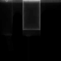
(b) SLAC

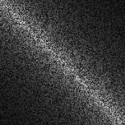
(c) Diagonal

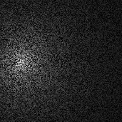
(d) Peak

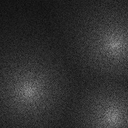
(e) Multi-peak

(f) Uniform

Figure 2: Examples of real and synthetic instances.

The SLAC dataset (depicted in Figure 2(b)) is generated from the mesh of a 3D object. Each vertex of the 3D object carries one unit of computation. Different instances can be generated by projecting the mesh on a 2D plane and by changing the granularity of the discretization. This setting match the experimental setting of [27]. In the experiments, we generated instances of size 512x512. Notice that the matrix contains zeroes, therefore $\Delta$ is undefined.

Different classes of synthetic squared matrices are also used, these classes are called diagonal, peak, multi-peak and uniform. Uniform matrices (Figure 2(f)) are generated to obtain a given value of $\Delta$: the computation load of each cell is generated uniformly between $1000$ and $1000*\Delta$. In the other three classes, the computation load of a cell is given by generating a number uniformly between 0 and the number of cells in the matrix which is divided by the Euclidean distance to a reference point (a 0.1 constant is added to avoid dividing by zero). The choice of the reference point is what makes the difference between the three classes of instances. In diagonal (Figure 2(c)), the reference point is the closest point on the diagonal of the matrix. In peak (Figure 2(d)), the reference point is one point chosen randomly at the beginning of the execution. In multi-peak (Figure 2(e)), several points (here 3) are randomly generated and the closest one will be the reference point. Those classes are inspired from the synthetic data from [24].

The performance of the algorithms is given using the load imbalance metric defined in Section 2. For synthetic dataset, the load imbalance is computed over 10 instances as follows: $\frac{\sum_{I}{L_{max}}(I)}{\sum_{I}{L_{avg}}(I)}-1$. The experiments are run on most square number of processors between 16 and 10,000. Using only square numbers allows us to fix the parameter $P=\sqrt{m}$ for all rectilinear and jagged algorithms.

4.2 Jagged algorithms

The jagged algorithms have three variants, two depending on whether the main dimension is the first one or the second one and the third tries both of them and takes the best solution. On all the fairly homogeneous instances (i.e., all but the mesh SLAC), the load imbalance of the three variants are quite close and the orientation of the jagged partitions does not seem to really matter. However this is not the same in $m$-way jagged algorithms where the selection of the main dimension can make significant differences on overall load imbalance. Since the $m$-way jagged partitioning heuristics are as fast as heuristic jagged partitioning, trying both dimensions and taking the one with best load imbalance is a good option. From now on, if the variant of a jagged partitioning algorithm is unspecified, we will refer to their BEST variant.

We proposed in Section 3.2.2 a new type of jagged partitioning scheme, namely, $m$-way jagged, which does not require all the slices of the main dimension to have the same number of processors. This constraint is artificial in most cases and we show that it significantly harms the load balance of an application.

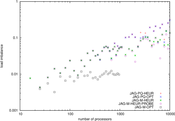
Figure 3: Jagged methods on PIC-MAG iter=30,000.

Figure 3 presents the load balance obtained on PIC-MAG at iteration 30,000 with heuristic and optimal $P\!\times\!Q$-way jagged algorithms and $m$-way jagged algorithms. On less than one thousand processors, JAG-M-HEUR, JAG-PQ-HEUR, JAG-PQ-OPT and JAG-M-HEUR-PROBE produce almost the same results (hence the points on the chart are super imposed). Note that, JAG-PQ-HEUR and JAG-PQ-OPT obtain the same load imbalance most of the time even on more than one thousand processors. This indicates that there is almost no room for improvement for the $P\!\times\!Q$-way jagged heuristic. JAG-M-HEUR-PROBE usually obtains the same load imbalance that JAG-M-HEUR or does slightly better. But on some cases, it leads to dramatic improvement. One can remark that the $m$-way jagged heuristics always reaches a better load balance than the $P\!\times\!Q$-way jagged partitions.

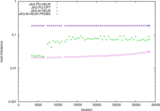
Figure 4: Jagged methods on PIC-MAG with $m=6400$.

Figure 4 presents the load imbalance of the algorithms with 6,400 processors for the different iterations of the PIC-MAG application. $P\!\times\!Q$-way jagged partitions have a load imbalance of 18% while the imbalance of the partitions generated by JAG-M-HEUR varies between 2.5% (at iteration 5,000) and 16% (at iteration 18,000). JAG-M-HEUR-PROBE achieves the best load imbalance of the heuristics between 2% and 3% on all the instances.

In Figure 3, the optimal $m$-way partition have been computed up to 1,000 processors (on more than 1,000 processors, the runtime of the algorithm becomes prohibitive). It shows an imbalance of about 1% at iteration 30,000 of the PIC-MAG application on 1,000 processors. This value is much smaller than the 6% imbalance of JAG-M-HEUR and JAG-M-HEUR-PROBE. It indicates that there is room for improvement for $m$-way jagged heuristics. Indeed, the current heuristic uses $\sqrt{m}$ parts in the first dimension, while the optimal is not bounded to that constraint. Notice that an optimal $m$-way partition with a given number of columns could be computed optimally using dynamic programming. Figure 5 presents the impact of the number of stripes on the load imbalance of JAG-M-HEUR on a uniform instance as well as the worst case imbalance of the $m$-way jagged heuristic guaranteed by Theorem 3. It appears clearly that the actual performance follows the same trend as the worst case performance of JAG-M-HEUR. Therefore, ideally, the number of stripes should be chosen according to the guarantee of JAG-M-HEUR. However, the parameters of the formula in Theorem 4 are difficult to estimate accurately and the variation of the load imbalance around that value can not be predicted accurately.

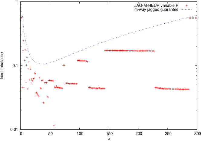
Figure 5: Impact of the number of stripes in JAG-M-HEUR on a 514x514 Uniform instance with $\Delta=1.2$ and $m=800$.

The load imbalance of JAG-PQ-HEUR, JAG-PQ-OPT, JAG-M-HEUR and JAG-M-HEUR-PROBE make some waves on Figure 3 when the number of processors varies. Those waves are caused by the imbalance of the partitioning in the main dimension of the jagged partition. Even more, these waves synchronized with the integral value of $\frac{n_{1}}{\sqrt{m}}$. This behavior is linked to the almost uniformity of the PIC-MAG dataset. The same phenomena induces the steps in Figure 5.

4.3 Hierarchical Bipartition

There are four variants of HIER-RB depending on the dimension that will be partitioned in two. In general the load imbalance increases with the number of processors. The HIER-RB-LOAD variant achieves a slightly smaller load balance than the HIER-RB-HOR, HIER-RB-VER and HIER-RB-DIST variants. The results are similar on all the classes of instances and are omitted.

There are also four variants to the HIER-RELAXED algorithm. Figure 6 shows the load imbalance of the four variants when the number of processors varies on the multi-peak instances of size 512. In general the load imbalance increases with the number of processors for HIER-RELAXED-LOAD and HIER-RELAXED-DIST. The HIER-RELAXED-LOAD variant achieves overall the best load balance. The load imbalance of the HIER-RELAXED-VER (and HIER-RELAXED-HOR) variant improves past 2,000 processors and seems to converge to the performance of HIER-RELAXED-LOAD. The number of processors where these variants start improving depends on the size of the load matrix. Before convergence, the obtained load balance is comparable to the one obtained by HIER-RELAXED-DIST. The diagonal instances with a size of 4,096 presented in Figure 7 shows this behavior.

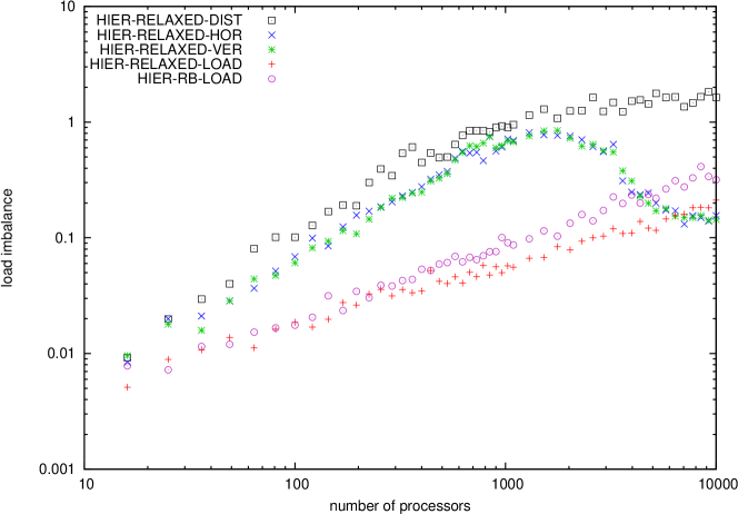
Figure 6: HIER-RELAXED on 512x512 Multi-peak.

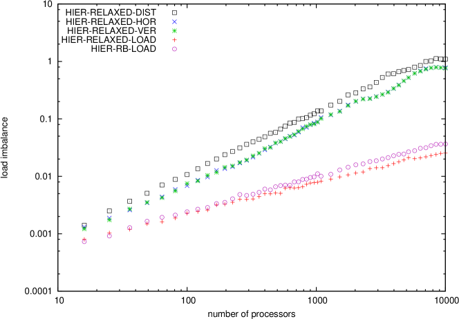
Figure 7: HIER-RELAXED on 4096x4096 Diagonal.

Since the load variant of both algorithm leads to the best load imbalance, we will refer to them as HIER-RB and HIER-RELAXED.

We proposed in Section 3.3, HIER-OPT, a dynamic programming algorithm to compute the optimal hierarchical bipartition. We did not implement HIER-OPT since we expect it to run in hours even on small instances. However, we derived HIER-RELAXED, from the dynamic programming formulation. Figure 6 and 7 include the performance of HIER-RB and allow to compare it to HIER-RELAXED. It is clear that HIER-RELAXED leads to a better load balance than HIER-RB in these two cases. However, the performance of HIER-RELAXED might be very erratic when the instance changes slightly. For instance, on Figure 8 the performance of HIER-RELAXED during the execution of the PIC-MAG application is highly unstable.

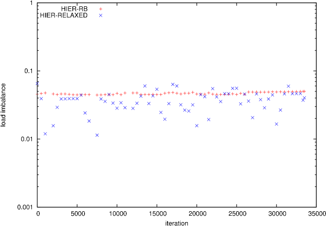
Figure 8: Hierarchical methods on PIC-MAG with $m=400$.

4.4 Execution time

In all optimization problems, the trade-off between the quality of a solution and the time spent computing it appears. We present in Figure 9 the execution time of the different algorithms on 512x512 Uniform instances with $\Delta=1.2$ when the number of processors varies. The execution times of the algorithms increase with the number of processors.

All the heuristics complete in less than one second even on 10,000 processors. The fastest algorithm is obviously RECT-UNIFORM since it outputs trivial partitions. The second fastest algorithm is HIER-RB which computes a partition in 10,000 processors in 18 milliseconds. Then comes the JAG-PQ-HEUR and JAG-M-HEUR heuristics which take about 106 milliseconds to compute a solution of the same number of processors. Notice that the execution of JAG-M-HEUR-PROBE takes about twice longer than JAG-M-HEUR. The running time of RECT-NICOL algorithm is more erratic (probably due to the iterative refinement approach) and it took 448 milliseconds to compute a partition in 10,000 rectangles. The slowest heuristic is HIER-RELAXED which requires 0.95 seconds of computation to compute a solution for 10,000 processors.

Two algorithms are available to compute the optimal $P\!\times\!Q$-way jagged partition. Despite the various optimizations implemented in the dynamic programming algorithm, JAG-PQ-OPT-DP is about one order of magnitude slower than JAG-PQ-OPT-NICOL. JAG-PQ-OPT-DP takes 63 seconds to compute the solution on 10,000 processors whereas JAG-PQ-OPT-NICOL only needs 9.6 seconds. Notice that using heuristic algorithm JAG-PQ-HEUR is two order of magnitude faster than JAG-PQ-OPT-NICOL, the fastest known optimal $P\!\times\!Q$-way jagged algorithm.

The computation time of JAG-M-OPT is not reported on the chart. We never run this algorithm on a large number of processors since it already took 31 minutes to compute a solution for 961 processors. The results on different classes of instances are not reported, but show the same trends. Experiments with larger load matrices show an increase in the execution time of the algorithm. Running the algorithms on matrices of size 8,192x8,192 basically increases the running times by an order of magnitude.

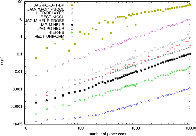
Figure 9: Runtime on 512x512 Uniform with $\Delta=1.2$.

Loading the data and computing the prefix sum array is required by all two dimensional algorithms. Hence, the time taken by these operations is not included in the presented timing results. For reference, it is about 40 milliseconds on a 512x512 matrix.

4.5 Which algorithm to choose?

The main question remains. Which algorithm should be chosen to optimize an application’s performance?

From the algorithm we presented, we showed that $m$-way jagged partitioning techniques provide better solutions than an optimal $P\!\times\!Q$-way jagged partition. It is therefore better than rectilinear partitions as well. The computation of an optimal $m$-way jagged partition is too slow to be used in a real system. It remains to decide between JAG-M-HEUR-PROBE, HIER-RB and HIER-RELAXED. As a point of reference, the results presented in this section also include the result of algorithm generating rectilinear partitioning, namely, RECT-UNIFORM and RECT-NICOL.

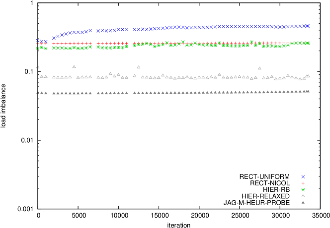
Figure 10: Main heuristics on PIC-MAG with $m=9216$.

Figure 10 shows the performance of the PIC-MAG application on 9,216 processors. The RECT-UNIFORM partitioning algorithm is given as a reference. It achieves a load imbalance that grows from 30% to 45%. RECT-NICOL reaches a constant 28% imbalance over time. HIER-RB is usually slightly better and achieves a load imbalance that varies between 20% and 30%. HIER-RELAXED achieves most of the time a much better load imbalance, rarely over 10% and typically between 8% and 9%. JAG-M-HEUR-PROBE outperforms all the other algorithms by providing a constant 5% load imbalance.

Figure 11 shows the performance of the algorithms while varying the number of processors at iteration 20,000. The conclusions on RECT-UNIFORM, RECT-NICOL and HIER-RB stand. Depending on the number of processors, the performance of JAG-M-HEUR-PROBE varies and in general HIER-RELAXED leads to the best performance, in this test.

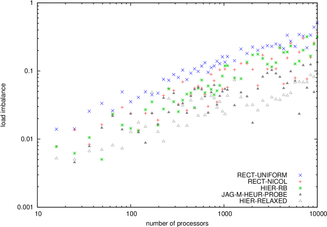
Figure 11: Main heuristics on PIC-MAG iter=20,000.

Figure 12 presents the performance of the algorithms on the mesh based instance SLAC. Due to the sparsity of the instance, most algorithms get a high load imbalance. Only the hierarchical partitioning algorithms manage to keep the imbalance low and HIER-RELAXED gets a lower imbalance than HIER-RB.

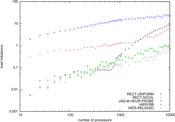
Figure 12: Main heuristics on SLAC.

The results indicate that as it stands, the algorithms HIER-RELAXED and JAG-M-HEUR-PROBE, we proposed, are the one to choose to get a good load balance. However, we believe a developer should be cautious when using HIER-RELAXED because of the erratic behavior it showed in some experiments (see Figure 8) and because of its not-that-low running time (up to one second on 10,000 processors according to Figure 9). JAG-M-HEUR-PROBE seems much a more stable heuristic. The bad load balance it presents on Figure 11 is due to a badly chosen number of partitions in the first dimension.

5 Hybrid partitioning scheme

The previous sections show that we have on one hand, heuristics that are good and fast, and on the other hand, optimal algorithms which are even better but to slow to be used in most practical cases. This section presents some engineering techniques one can use to obtain better results than using only the heuristics while keeping the runtime of the algorithms reasonable.

Provided, in general the maximum load of a partition is given by the most loaded rectangle and not by the general structure of the partition, one idea is to use the optimal algorithm to be locally efficient and leave the general structure to a faster algorithm. We introduce the class of HYBRID algorithms which construct a solution in two phases. A first algorithm will be used to partition the matrix $A$ in $P$ parts. Then the parts will be independently partitioned with a second algorithm to obtain a solution in $m$ parts. This section investigates the hybrid algorithms and try to answer the following questions: Which algorithms should be used at phase 1 and phase 2? In how many parts the matrix should be divided in the first phase (i.e., what should $P$ be)? How to allocate the $m$ processors between the $P$ parts? And most importantly, is there any advantage in using hybrid algorithms?

Between the two phases, it is difficult to know how to allocate the $m$ processors to the $P$ parts without doing a deep search. We choose to allocate the parts proportionally according to the rule used in JAG-M-HEUR, i.e., each rectangle $r$ will first be allocated $Q_{r}=\lceil\frac{L(r)}{L(A)}(m-P)\rceil$ parts. The remaining processors are distributed greedily.

We conducted experiments using different PIC-MAG instances. All the values of $P$ were tried between $2$ and $\frac{m}{2}$. We will denote the HYBRID algorithm using ALGO1 for phase 1 and ALGO2 for phase 2 as HYBRID(ALGO1/ALGO2).

The first round of experiments mainly showed three observations. (No results are shown since similar results will be presented later.) First, HYBRID is too slow to use JAG-M-OPT at the second phase for studying the performance (e.g., partitioning PIC-MAG at iteration 5000 on $1024$ processors using $P=17$ takes $78$ seconds). Second, the performance shows ”waves” when $P$ varies which are correlated with the values of $\lceil\frac{m-P}{P}\rceil$. Finally HYBRID can obtain load imbalances better than JAG-M-HEUR and HIER-RELAXED on some configuration confirming that HYBRID might be useful.

To make the algorithm faster, we introduce the notion of fast and slow algorithms at phase 2. The fast algorithm is first run on each part and the parts are sorted according to their maximum load. The slow algorithm is run on the part of higher maximum load. If the solution returned by the slow algorithm improves the maximum load of that part, the solution is kept and the parts are sorted again. Otherwise, the algorithm terminates. This modification increased the speed of the algorithm up to an order of magnitude. (Using JAG-M-HEUR-PROBE as the fast algorithm in phase 2 allows to run PIC-MAG at iteration 5000 on $1024$ processors using $P=17$ in $38$ seconds, halving the computation time.) Detailed timing on PIC-MAG at iteration 5000 using $1024$ processors can be found in Figure 13. The HYBRID(JAG-M-HEUR/JAG-M-OPT) curve is the original implementation of HYBRID using JAG-M-HEUR at phase 1 and JAG-M-OPT at phase 2. The HYBRID-F(JAG-M-HEUR/JAG-M-OPT) curve presents the timing obtained with the use of fast and slow algorithm. The HYBRID algorithm using JAG-M-OPT at both phase is given as a point of reference. All the implementation used JAG-M-HEUR-PROBE as the fast algorithm. Figure 13 shows that using fast and slow algorithms makes the computation about one order of magnitude faster. Using JAG-M-OPT at phase 1 is typically orders of magnitude slower than using another algorithm.

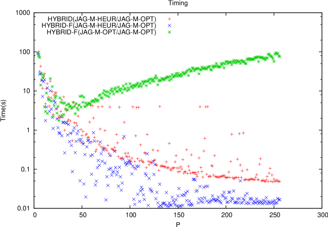
Figure 13: Runtime of HYBRID methods on PIC-MAG iter=5000 with $m=512$.

This improvement allows to run more complete and detailed experiments. In particular, using JAG-M-OPT at phase 2 runs quickly. This allow us to study the performance of HYBRID using an algorithm that get good load balance at phase 2. The load imbalance obtained on PIC-MAG 5000 on $512$ are shown in Figure 14. Two HYBRID variants that use JAG-M-OPT or HIER-RELAXED at phase 1 are presented. For reference, three horizontal lines present the performance obtained by JAG-M-HEUR, HIER-RELAXED and JAG-M-OPT on that instance. A first remark is that a large number of configurations lead to load imbalances better than JAG-M-HEUR. A significant number of them get load imbalances better than HIER-RELAXED and sometimes comparable to the performance of JAG-M-OPT. Then, the load imbalance significantly varies with $P$: it is decreasing by interval which happen to be synchronized with the values of $\lceil\frac{m-P}{P}\rceil$. Finally, the load imbalance is better when the values of $P$ are low. This behavior was predictable since the lower $P$ is the more global the optimization is. However, one should notice that some low load imbalances are found with high values of $P$.

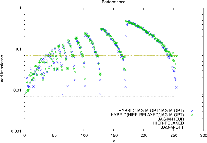
Figure 14: Using JAG-M-OPT at phase 2 on PIC-MAG iter=5000 with $m=512$

Good load imbalance could obviously be obtained by trying every single value of $P$. However, such a procedure is likely to take a lot of time. Provided the phase 2 algorithm takes a large part of the computation time, it will be interesting to predict the performance of the second phase without having to run it. We define the expected load imbalance as the load imbalance that would be obtained provided the second phase balances the load optimally, i.e., $eLI=\max_{r}\frac{L(r)}{Q_{r}}$. Figure 15 presents for each solution its expected load imbalance and the load imbalance obtained once the second phase is run for different values of $P$. The solutions are presented for two hybrid variants, one using JAG-M-HEUR at phase 2 and the other one using JAG-M-OPT. For similar expected load imbalance, the load imbalance obtained using JAG-M-HEUR are spread over an order of magnitude. However, the load imbalance obtained by JAG-M-OPT are much more focused. The expected load imbalance and obtained load imbalance are well correlated when JAG-M-OPT is used at phase 2.

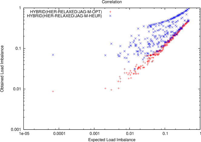
Figure 15: Correlation between expected load imbalance at the end of phase 1 and the obtained load imbalance on PIC-MAG iter=5000 with $m=512$

The previous experiments show two things. The actual performance are correlated with expected performance at the end of phase 1 if JAG-M-OPT is used in phase 2. The load imbalance decreases in an interval of values of $P$ synchronized with the values of $\lceil\frac{m-P}{P}\rceil$. Therefore, we propose to enumerate the values of $P$ at the end of such intervals. For each of these value, the phase 1 algorithm is used and the expected load imbalance is computed. The phase 2 is only applied on the value of $P$ leading to the best expected load imbalance. Obviously the best expected load imbalance will be given by the non-hybrid case $P=1$, but it will lead to a high runtime. The tradeoff between the runtime of the algorithm and the quality of the solution should be left to the user by specifying a minimal $P$.

Figure 16 presents the load imbalance obtained on the PIC-MAG datasets at iteration 10000 using $\sqrt{m}$ as minimal $P$. The HYBRID algorithm obtains a load balance usually better than JAG-M-HEUR-PROBE and often better than HIER-RELAXED. The algorithm leading to the best load imbalance seems to depend on the number of processors. For instance, Figure 17 shows the load imbalance of the algorithms on 7744 processors. JAG-M-HEUR-PROBE leads constantly to better results than HIER-RELAXED. And HYBRID typically improve both by a few percents.

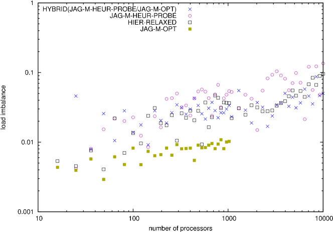
Figure 16: HYBRID algorithm on PIC-MAG iter=10000

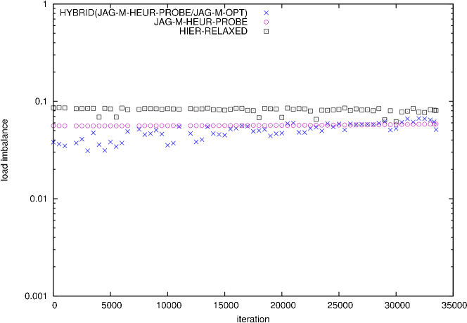
Figure 17: HYBRID algorithm on PIC-MAG on 7744 processors

However, on 6400 processors (Figure 18), HYBRID almost constantly improves the result of HIER-RELAXED by a few percents but does not achieve better load imbalance than JAG-M-HEUR-PROBE. Figure 4 showed that JAG-M-HEUR is significantly outperformed by JAG-M-HEUR-PROBE in that configuration. Recall that the main difference between these heuristics is that the former distributes the processors among the stripes only based on the load of each stripe while the latter use the minimum number of processors per stripe to obtain the minimum load balance. The same idea could be applied to HYBRID algorithms looking for the minimum number of processors to allocate to each part without degrading the load imbalance and use these processors on the parts that lead to the maximum load. This modification will improve the load imbalance but will also increase the running time significantly.

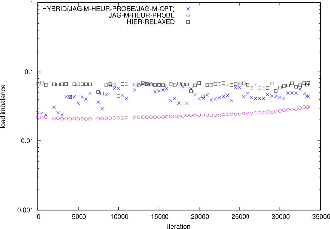
Figure 18: HYBRID algorithm on PIC-MAG on 6400 processors

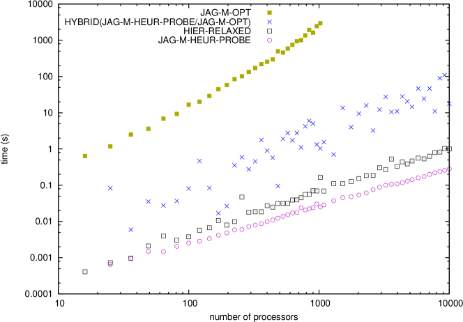
Figure 19: Runtime of HYBRID methods on PIC-MAG iter=10000

The runtime of the algorithm is presented in Figure 19. It shows that the HYBRID algorithm is two or three orders of magnitude slower than the heuristics but one to two orders of magnitude faster than JAG-M-OPT. However, HYBRID algorithms are likely to parallelize pleasantly.

Some more engineering techniques could be applied to HYBRID. Different time/quality tradeoff could be obtained by stopping the use of the slow algorithm in phase 2 when the improvement become smaller than a given threshold. Using a 3-phase HYBRID mechanism could be another way of obtaining different trade-offs.

HYBRID is not the only option for algorithm engineering. One idea that might lead to interesting time/quality tradeoff would be to avoid running dynamic programming algorithms all the way through. Early termination can be decided based on a time allocation or a targeted maximum load.

Finally, different kind of iterative improvement algorithms could be designed. For instance, on $m$-way jagged partition, JAG-M-PROBE provides the optimal number of processors to use in each stripe provided the partition in the main dimension, and JAG-M-ALLOC provides the optimal partition in the main dimension provided the number of processors allocated to each stripe. Applying JAG-M-PROBE and JAG-M-ALLOC the one after the other as long as the solution improves would be one interesting iterative algorithm.

6 Conclusion

Partitioning spatially localized computations evenly among processors is a key step in obtaining good performance in a large class of parallel applications. In this work, we focused on partitioning a matrix of non-negative integers using rectangular partitions to obtain a good load balance. We introduced the new class of solutions called $m$-way jagged partitions, designed polynomial optimal algorithms and heuristics for $m$-way partitions. Using theoretical worst case performance analyses and simulations based on logs of two real applications and synthetic data, we showed that the JAG-M-HEUR-PROBE and HIER-RELAXED heuristics we proposed get significantly better load balances than existing algorithms while running in less than a second. We showed how HYBRID algorithms can be engineered to achieve better load balance but use significantly more computing time. Finally, if computing time is not really a limitation, one can use more complex algorithm such that JAG-M-OPT.

Showing that the optimal solution for $m$-way jagged partitions, hierarchical bipartitions and hierarchical $k$-partitions with constant $k$ can be computed in polynomial time is a strong theoretical result. However, the runtime complexity of the proposed dynamic programming algorithm remains high. Reducing the polynomial order of these algorithms will certainly be of practical interest.

We only considered computations located in a two dimensional field but some applications, such as PIC-MAG and SLAC, might expose three or more dimensions. A simple way of dealing with higher dimension would be to project the space in two dimensions and using a two dimensional partitioning algorithm, as we have done in some of the applications. But this choice is likely to be suboptimal since it drastically restrict the set of possible allocations. An alternative would be to extend the classes of partitions and algorithm to higher dimension. For instance, a jagged partitioning algorithm would partition the space along one dimension and perform a projection to obtain planes which will be partitioned in stripes and projected to one dimensional arrays partitioned in intervals. All the presented algorithms extend in more than two dimensions, therefore the problems will stay in the same complexity class. However, the guaranteed approximation is likely to worsen, the time complexity is likely to increase (especially for dynamic programming based algorithms). Memory occupation is also likely to become an issue and providing cache efficient algorithm should be investigated. However, the increase of the size of the solution space will provide better load balance than partitioning the two dimensional projection.

We are also planning to integrate the proposed algorithms in a distributed particle in cell simulation code. To optimize the application performance, we will need to take into account communication into account while partitioning the task. Dynamic application will require rebalancing and the partitioning algorithm should take into account data migration cost. Finally, to keep the rebalancing time as low as possible, it might useful not to gather the load information on one machine but to perform the repartitioning using a distributed algorithm.

References

- [1] A. Abdelkhalek and A. Bilas. Parallelization and performance of interactive multiplayer game servers. In Proc. of IPDPS, 2004.
- [2] M. Aftosmis, M. Berger, and S. Murman. Applications of space filling curves to cartesian methods for CFD. In Proc. of the 42nd AIAA Aerospace Sciences Meeting, 2004.
- [3] S. Aluru and F. E. Sevilgen. Parallel domain decomposition and load balancing using space-filling curves. In Proc. of the 4th IEEE Conference on High Performance Computing, pages 230–235, 1997.
- [4] B. Aspvall, M. M. Halldórsson, and F. Manne. Approximations for the general block distribution of a matrix. Theoretical Computer Science, 262(1-2):145–160, 2001.
- [5] M. Berger and S. Bokhari. A partitioning strategy for nonuniform problems on multiprocessors. IEEE Transactions on Computers, C36(5):570–580, 1987.
- [6] S. H. Bokhari. Partitioning problems in parallel, pipeline, and distributed computing. IEEE Transactions on Computers, 37(1):48–57, 1988.
- [7] U. V. Çatalyürek and C. Aykanat. Hypergraph-partitioning based decomposition for parallel sparse-matrix vector multiplication. IEEE Transactions on Parallel and Distributed Systems, 10(7):673–693, 1999.
- [8] U. V. Çatalyürek, E. Boman, K. Devine, D. Bozdag, R. Heaphy, and L. Fisk. A repartitioning hypergraph model for dynamic load balancing. Journal of Parallel and Distributed Computing, 69(8):711–724, 2009.
- [9] J. E. Flaherty, R. M. Loy, M. S. Shephard, B. K. Szymanski, J. D. Teresco, and L. H. Ziantz. Adaptive local refinement with octree load-balancing for the parallel solution of three-dimensional conservation laws. Journal of Parallel and Distributed Computing, 47:139–152, 1997.
- [10] H. P. F. Forum. High performance FORTRAN language specification, version 2.0. Technical Report CRPC-TR92225, CRPC, Jan. 1997.
- [11] G. N. Frederickson. Optimal algorithms for partitioning trees and locating p-centers in trees. Technical Report CSD-TR-1029, Purdue University, 1990, revised 1992.
- [12] D. R. Gaur, T. Ibaraki, and R. Krishnamurti. Constant ratio approximation algorithms for the rectangle stabbing problem and the rectilinear partitioning problem. Journal of Algorithms, 43(1):138–152, 2002.
- [13] M. Grigni and F. Manne. On the complexity of the generalized block distribution. In Proc. of IRREGULAR ’96, pages 319–326, 1996.
- [14] Y. Han, B. Narahari, and H.-A. Choi. Mapping a chain task to chained processors. Information Processing Letter, 44:141–148, 1992.
- [15] B. Hendrickson and T. G. Kolda. Graph partitioning models for parallel computing. Parallel Computing, 26:1519–1534, 2000.
- [16] V. Horak and P. Gruber. Parallel numerical solution of 2D heat equation. In Parallel Numerics ’05, pages 47–56, 2005.
- [17] H. Karimabadi, H. X. Vu, D. Krauss-Varban, and Y. Omelchenko. Global hybrid simulations of the earth’s magnetosphere. Numerical Modeling of Space Plasma Flows, Dec. 2006.
- [18] S. Khanna, S. Muthukrishnan, and M. Paterson. On approximating rectangle tiling and packaging. In Proc. of the 19th SODA, pages 384–393, 1998.
- [19] S. Khanna, S. Muthukrishnan, and S. Skiena. Efficient array partitioning. In Proc. of ICALP ’97, pages 616–626, 1997.
- [20] H. Kutluca, T. Kurc, and C. Aykanat. Image-space decomposition algorithms for sort-first parallel volume rendering of unstructured grids. Journal of Supercomputing, 15:51–93, 2000.
- [21] A. L. Lastovetsky and J. J. Dongarra. Distribution of computations with constant performance models of heterogeneous processors. In High Performance Heterogeneous Computing, chapter 3. John Wiley & Sons, 2009.
- [22] J. Y.-T. Leung. Some basic scheduling algorithms. In J. Y.-T. Leung, editor, Handbook of Scheduling, chapter 3. CRC Press, 2004.
- [23] F. Manne and B. Olstad. Efficient partitioning of sequences. IEEE Transactions on Computers, 44(11):1322–1326, 1995.
- [24] F. Manne and T. Sørevik. Partitioning an array onto a mesh of processors. In Proc of PARA ’96, pages 467–477, 1996.
- [25] S. Miguet and J.-M. Pierson. Heuristics for 1d rectilinear partitioning as a low cost and high quality answer to dynamic load balancing. In Proc. of HPCN Europe ’97, pages 550–564, 1997.
- [26] S. Muthukrishnan and T. Suel. Approximation algorithms for array partitioning problems. Journal of Algorithms, 54:85–104, 2005.
- [27] D. Nicol. Rectilinear partitioning of irregular data parallel computations. Journal of Parallel and Distributed Computing, 23:119–134, 1994.
- [28] K. Paluch. A new approximation algorithm for multidimensional rectangle tiling. In Proc. of ISAAC, 2006.
- [29] J. R. Pilkington and S. B. Baden. Dynamic partitioning of non-uniform structured workloads with spacefilling curves. IEEE Transactions on Parallel and Distributed Systems, 7(3):288–300, 1996.
- [30] A. Pınar and C. Aykanat. Sparse matrix decomposition with optimal load balancing. In Proc. of HiPC 1997, 1997.
- [31] A. Pınar and C. Aykanat. Fast optimal load balancing algorithms for 1D partitioning. Journal of Parallel and Distributed Computing, 64:974–996, 2004.
- [32] A. Pınar, E. Tabak, and C. Aykanat. One-dimensional partitioning for heterogeneous systems: Theory and practice. Journal of Parallel and Distributed Computing, 68:1473–1486, 2008.
- [33] S. J. Plimpton, D. B. Seidel, M. F. Pasik, R. S. Coats, and G. R. Montry. A load-balancing algorithm for a parallel electromagnetic particle-in-cell code. Computer Physics Communications, 152(3):227 – 241, 2003.
- [34] E. Saule, E. O. Bas, and Ümit V. Çatalyürek. Partitioning spatially located computations using rectangles. In Proc. of IPDPS, 2011.
- [35] K. Schloegel, G. Karypis, and V. Kumar. A unified algorithm for load-balancing adaptive scientific simulations. In Proc. of SuperComputing ’00, November 2000.
- [36] M. Ujaldon, S. Sharma, E. Zapata, and J. Saltz. Experimental evaluation of efficient sparse matrix distributions. In Proc. of SuperComputing’96, 1996.
- [37] B. Vastenhouw and R. H. Bisseling. A two-dimensional data distribution method for parallel sparse matrix-vector multiplication. SIAM Review, 47(1):67–95, 2005.