Nontrival Cosmological Constant in Brane Worlds with Unorthodox Lagrangians

Stefan Förste, Hans Peter Nilles, Ivonne Zavala

Bethe Center for Theoretical Physics
and
Physikalisches Institut der Universität Bonn,
Nussallee 12, 53115 Bonn, Germany

Abstract

In self-tuning brane-world models with extra dimensions, large contributions to the cosmological constant are absorbed into the curvature of extra dimensions and consistent with flat 4d geometry. In models with conventional Lagrangians fine-tuning is needed nevertheless to ensure a finite effective Planck mass. Here, we consider a class of models with non conventional Lagrangian in which known problems can be avoided. Unfortunately these models are found to suffer from tachyonic instabilities. An attempt to cure these instabilities leads to the prediction of a positive cosmological constant, which in turn needs a fine-tuning to be consistent with observations.

1 Introduction

Quantum corrections to the cosmological constant are of the order $M_{p}^{4}$ where $M_{p}$ denotes the Planck mass. To achieve agreement with observations that the cosmological constant is less than $10^{-120}M_{p}^{4}$ requires a severely fine-tuned bare value. (With supersymmetry broken below the Planck scale the fine-tuning is slightly relaxed but cannot be sufficiently removed.) Reviews on the cosmological constant problem are e.g. listed in [1, 2, 3, 4].

About ten years ago, the fine-tuning problem was revisited in the context of brane-worlds. The basic idea is that some extra directions can be probed only by gravitational interactions and are thus not visible to us. Vacuum energy created by matter and the other interactions could curve the extra dimension and would not be observable. Famous examples in which such a picture is realised are the Randall-Sundrum (RS) models [5, 6]. There, however, the fine-tuning appears in matching conditions between bulk and brane parameters [5, 6, 7]. Later it was proposed to add a bulk scalar field in order to avoid this fine-tuning [8, 9]. Indeed, the matching condition between bulk and brane parameters just fixes integration constants and thus self-tuning is apparently achieved. However, to avoid singularities and to get a finite value for the Planck mass one needs to cut-off the extra dimension. This can be done consistently only by adding branes with fine-tuned tensions [10, 11]. It can be shown that this problem persists for quite general bulk potentials of the scalar [12].

The authors of [13] proposed an interesting model which circumvents all these known problems. It has an unconventional kinetic term, expansion around a vacuum configuration results in a higher derivative model. (For subsequent work on this model see [14] and references therein.) A quite different analysis also hints at unconventional bulk Lagrangians to be needed for a working self-tuning mechanism [15, 16]. (Their conditions however seem to differ from the ones in [13] and the ones considered in the present article.)

We will describe a class of models in which a bulk scalar has an unconventional kinetic term. These models can also be seen as a natural generalisation of RS [5, 6] and [8, 9], which are contained in our set up. These models have a single brane, matching conditions just fix integration constants, singularities are avoided and the Planck mass will be finite without introducing extra branes. A stability analysis shows that perturbations depending on the extra coordinate are indeed damped in one class of models, while to achieve damping of fluctuations depending on the visible directions fine-tuning has to be reintroduced. The class of models discussed here contains the model in [13] in its dual formulation [17]. In this case, perturbations depending on the visible coordinates are damped, while fluctuations depending on the extra dimension give rise to tachyonic Kaluza Klein (KK) masses. Attempts to cancel such negative mass-squareds lead to the prediction that the cosmological constant has to be nonzero and positive. Unfortunately the size of the cosmological constant is again a subject of fine-tuning.

We will not consider more than one extra dimension. Examples with two extra dimensions are discussed in [19, 20, 21, 22, 23, 24, 25, 26, 27, 28] (where especially [24, 25, 26] provide a critical evaluation of self-tuning proposals).

The paper is organised as follows. In the next section we construct self-tuning solutions with one extra dimension. The kinetic term of a bulk scalar is raised to a real power $\alpha$. Conditions on $\alpha$ from imposing a finite effective Planck mass are derived in section 3. As a crosscheck we compute the effective cosmological constant in section 4 and give an estimated lower bound on the size of the extra dimension. In section 5 we show that imposing stability enforces non vanishing effective cosmological constant and reintroduces a fine-tuning condition. Section 6 discusses nearby curved solution. In section 7, we argue that the problems persist upon adding a bulk cosmological constant. In section 8 we relate our class of models to models with a three-form potential via electric magnetic duality. In section 9 we summarize our results.

2 “Self-Tuning” with Unconventional Lagrangian

The system we consider consists of a bulk action and a brane action

$$S=S_{\text{bulk}}+S_{\text{brane}},$$

with

$$S_{\text{bulk}}=\int d^{4}xdy\sqrt{-G}\left(\frac{R}{2\kappa_{5}^{2}}-\lambda\left(\partial_{M}\Phi\partial^{M}\Phi^{\dagger}\right)^{\alpha}\right)$$ (1)

and

$$S_{\text{brane}}=-\int d^{4}x\sqrt{-g}f\left(\Phi\right)_{\left|y=0\right.}.$$ (2)

Here, $G_{MN}$ is the five dimensional metric. The fifth coordinate is called $y$ and the 4d coordinates are $x^{\mu}$, $\mu=0,\ldots,3$. Moreover, the parameters $\lambda$ and $\alpha$ are for the moment arbitrary. Notice that the self-tuning system discussed in [8] can be recovered from (1) by taking $\lambda=4/3$ and $\alpha=1$, which indeed corresponds to a bulk scalar field with standard kinetic term. Moreover, the RS solution [5, 6] is recovered for $\alpha=0$ and $\lambda=1$, which corresponds simply to a bulk cosmological constant. Thus it is reasonable to consider as an interpolating scheme the more general system above with arbitrary $\alpha$.

The brane is taken to be localised within the fifth dimension at $y=0$. Then the induced metric on the brane reads

$$g_{\mu\nu}=G_{MN}\delta^{M}_{\mu}\delta^{N}_{\nu\left|y=0\right.},\quad\mu,\nu=0,\ldots,3.$$ (3)

We have taken a complex scalar to have single valuedness of the action under $\Phi\to e^{2\pi\mbox{\scriptsize i}}\Phi$. The differences to a real field turn out to be less important. For the metric we take an ansatz compatible with 4d Minkowski isometry

$$ds^{2}=a\left(y\right)^{2}\eta_{\mu\nu}\,dx^{\mu}dx^{\nu}+dy^{2},$$ (4)

where $\eta_{\mu\nu}=diag\left(-1,1,1,1\right)$ is the Minkowski metric. The equations of motion are

$$6\left(\frac{a^{\prime}}{a}\right)^{2}=\kappa_{5}^{2}\lambda\left(2\alpha-1\right)\left|\Phi^{\prime}\right|^{2\alpha}$$ (5)

from the $yy$ component of Einstein’s equation. We allow at most for $y$ dependence and denote the corresponding derivatives with a prime. The $\mu\nu$ components of Einstein’s equation give rise to

$$3\frac{a^{\prime\prime}}{a}=-\frac{\lambda\kappa_{5}^{2}}{2}\left(2\alpha+1\right)\left|\Phi^{\prime}\right|^{2\alpha}-f\left(\Phi\right)\delta\left(y\right)\kappa_{5}^{2}.$$ (6)

Finally, the equation for the complex scalar reads

$$\frac{\lambda\alpha}{a^{4}}\left(a^{4}\left|\Phi^{\prime}\right|^{2\left(\alpha-1\right)}\Phi^{\prime}\right)^{\prime}=\frac{\partial f}{\partial\Phi^{\dagger}}\delta\left(y\right).$$ (7)

We proceed now to solve these equations. From the Einstein equation (5) we get

$$\frac{a^{\prime}}{a}=\pm A\left|\Phi^{\prime}\right|^{\alpha}$$ (8)

with

$$A=\sqrt{\frac{\kappa_{5}^{2}\lambda\left(2\alpha-1\right)}{6}}.$$ (9)

Reality of $a$ forces us to take the parameters $\lambda$ and $\alpha$ such that the argument under the square root is real and positive, i.e.

$$\lambda\left(2\alpha-1\right)>0$$ (10)

Therefore we have two types of solutions: a) $\alpha>1/2,\,\lambda>0$ (the solutions in [8] fall into this class and one could then suspect the appearance of singularities) and b) $\alpha<1/2,\,\lambda<0$. As we see below case b) is the most interesting one from the point of view of a realisation of the self-tuning mechanism.

We pick the branch of the root such that $A>0$. Using this in the scalar equation (7) and combining with its complex conjugate we obtain

$$\lambda\alpha\left|\Phi^{\prime}\right|^{2\alpha}\left(\frac{\Phi^{\prime\prime}}{\Phi^{\prime}}-\frac{{\Phi^{\dagger}}^{\prime\prime}}{{\Phi^{\dagger}}^{\prime}}\right)=\left({\Phi^{\dagger}}^{\prime}\frac{\partial f}{\partial\Phi^{\dagger}}-\Phi^{\prime}\frac{\partial f}{\partial\Phi}\right)\delta\left(y\right).$$ (11)

For $y\not=0$ this is solved by

$$\Phi^{\prime}=e^{\mbox{\scriptsize i}\rho}\varphi^{\prime},$$ (12)

where $\rho$ is a real integration constant (which can jump at $y=0$) and $\varphi$ is a real $y$ dependent field. Further we disregard the possibility of having constant $\Phi$ since that leads to a constant warp factor. A constant warp factor either results in a divergent effective Planck mass or one has to introduce more branes to compactify the fifth direction by cutting it off. The equation for the remaining real scalar $\varphi$ is

$$\lambda\alpha\left|\varphi\right|^{2\alpha}\left(\left(2\alpha-1\right)\frac{\varphi^{\prime\prime}}{\varphi^{\prime}}\pm 4A\left|\varphi^{\prime}\right|^{\alpha}\right)=e^{-\mbox{\scriptsize i}\rho}\varphi^{\prime}\frac{\partial f}{\partial\Phi^{\dagger}}\delta\left(y\right).$$ (13)

For $y\not=0$ this leads to

$$e^{-\alpha\log\left|\varphi^{\prime}\right|}=\left|\varphi^{\prime}\right|^{-\alpha}=\pm\frac{4\alpha A\,y}{2\alpha-1}+C_{1},$$ (14)

where $C_{1}$ is a real integration constant which can again change at $y=0$. The left hand side of (14) is never negative. Curvature singularities at finite $y$ can be avoided if the right hand side does not change sign. So, we take

$$C_{1}\geq 0.$$ (15)

The first term on the right hand side of (14) should neither be negative. So, for instance if (this will turn out to be the case of interest below)

$$\frac{\alpha}{2\alpha-1}<0$$ (16)

we take the lower sign for $y>0$ and the upper sign for $y<0$. The complete solution for the complex scalar is then

$$\Phi=-\frac{\Theta\left(y\right)\left(2\alpha-1\right)}{4A\left(\alpha-1\right)}e^{\mbox{\scriptsize i}\rho}\left(-\frac{4\,\alpha A}{2\alpha-1}\left|y\right|+C_{1}\right)^{\frac{\alpha-1}{\alpha}}+C_{2},$$ (17)

where $C_{2}$ is a complex integration constant and $\Theta\left(y\right)$ denotes the Heaviside step function. Solving Einstein’s equations for $y\not=0$ yields the warp factor

$$a=\left(C_{3}\left(-\frac{4\,\alpha A}{2\alpha-1}\left|y\right|+C_{1}\right)\right)^{\frac{2\alpha-1}{4\alpha}}.$$ (18)

Analysing our set of equations at $y=0$ one finds that $\Phi$ and $a$ should be continuous. Denoting the value of an integration constant at $y\gtrless 0$ by a superscript $\pm$ we find from imposing continuity of $\Phi$ and $a$

$$-\frac{2\alpha-1}{4A\left(\alpha-1\right)}e^{\text{i}\rho^{+}}\left(C_{1}^{+}\right)^{\frac{\alpha-1}{\alpha}}+C_{2}^{+} =\frac{2\alpha-1}{4A\left(\alpha-1\right)}e^{\text{i}\rho^{-}}\left(C_{1}^{-}\right)^{\frac{\alpha-1}{\alpha}}+C_{2}^{-},$$ (19)

$$\left(C_{3}^{+}C_{1}^{+}\right)^{\frac{2\alpha-1}{4\alpha}} =\left(C_{3}^{-}C_{1}^{-}\right)^{\frac{2\alpha-1}{4\alpha}}.$$ (20)

First derivatives have to jump by a finite amount such that second derivatives reproduce the delta function on the right hand side of the equations of motion. This leads to the following jump conditions on the integration constants

$$\lambda\,\alpha\left(e^{\text{i}\rho^{+}}\left(C_{1}^{+}\right)^{\frac{1-2\alpha}{\alpha}}-e^{\text{i}\rho^{-}}\left(C_{1}^{-}\right)^{\frac{1-2\alpha}{\alpha}}\right) =\frac{\partial f}{\partial\Phi^{\dagger}},$$ (21)

$$\frac{1}{C_{1}^{+}}+\frac{1}{C_{1}^{-}}=\frac{\kappa_{5}^{2}f\left(\Phi\right)}{3A}.$$ (22)

From our earlier finding that $C_{1}\geq 0$ and (22) we see that the solution with 4d Minkowski isometry exists for any value of a positive cosmological constant on the brane. This is the so-called “self-tuning” mechanism. (The quotation marks indicate that the solution still has to pass some consistency condition to be discussed subsequently.)

3 Effective Planck Mass

The effective four dimensional Planck mass, $M_{p}$, can be obtained as follows. We replace the 4d Minkowski metric in (4) by a general $x$ dependent metric, plug that into the bulk action (1) and integrate over the fifth dimension. The result contains a 4d Einstein-Hilbert term, the factor in front of which yields the effective 4d gravitational coupling, $\kappa$. One obtains

$$\frac{1}{\kappa}=\frac{M_{p}^{2}}{8\pi}=\frac{1}{\kappa_{5}^{2}}\int dy\,a^{2}$$ (23)

With our solution (18) we get

$$\frac{\kappa_{5}^{2}}{\kappa}=\int_{-y_{c}}^{y_{c}}dy\left(C_{3}\left(-\frac{\alpha 4A}{2\alpha-1}\left|y\right|+C_{1}\right)\right)^{\frac{2\alpha-1}{2\alpha}} =$$

$$\left.-\frac{2\alpha-1}{2A\left(4\alpha-1\right)}\frac{\Theta\left(y\right)}{C_{3}}\left(C_{3}\left(-\frac{\alpha 4A}{2\alpha-1}\left|y\right|+C_{1}\right)\right)^{\frac{4\alpha-1}{2\alpha}}\right|^{y_{c}}_{y=-y_{c}},$$ (24)

where we have cut off the integration at $y=\pm y_{c}$. To consistently do so one would need to introduce additional branes with fine-tuned tension at those positions [10, 11]. Such fine-tuning can be avoided while obtaining finite Planck mass when the limit $y_{c}\to\infty$ is finite. This leads to the condition

$$0<\alpha<\frac{1}{4}.$$ (25)

Thus we see that solution b) $\alpha<1/2,\,\lambda<0$ is the only one which could give rise to a successful self-tuning mechanism. Notice that the region between $1/4<\alpha<1/2$ is excluded due to the requirement of finiteness of the Planck mass (see Fig. 1). We see below that adding a bulk cosmological constant can help in allowing this region.

If (25) holds, the four dimensional gravitational coupling is given by

$$\frac{\kappa_{5}^{2}}{\kappa}=\frac{2\alpha-1}{2A\left(4\alpha-1\right)}\left(C_{3}C_{1}\right)^{\frac{4\alpha-1}{2\alpha}}\left(\frac{1}{C_{3}^{+}}+\frac{1}{C_{3}^{-}}\right),$$ (26)

where we used the continuity of $C_{1}C_{3}$ (20).

4 Cross Check: Effective 4d Cosmological Constant

Since 4d slices in our five dimensional brane world are flat, the effective cosmological constant should vanish. It is computed as the Lagrangian evaluated at the solution and integrated over the fifth direction,

$$\Lambda_{\text{eff}}=\int_{-y_{c}}^{y_{c}}dy\,a^{4}\left(-\frac{4a^{\prime\prime}}{\kappa_{5}^{2}a}-\frac{6}{\kappa_{5}^{2}}\left(a^{\prime}{a}\right)^{2}-\lambda\left|\Phi^{\prime}\right|^{2\alpha}\right)-a^{4}f_{\left|y=0\right.}.$$ (27)

Plugging in our solution, taking carefully into account delta function contributions to second derivatives, we find

$$\Lambda_{\text{eff}}=\left.\left(C_{3}\right)^{\frac{2\alpha-1}{\alpha}}\frac{\lambda}{6A}\Theta\left(y\right)\left(-\frac{\alpha 4A}{2\alpha-1}\left|y\right|+C_{1}\right)^{\frac{\alpha-1}{\alpha}}\right|_{y=-y_{c}}^{y_{c}}+\frac{1}{3}\left(C_{3}C_{1}\right)^{\frac{2\alpha-1}{\alpha}}f.$$ (28)

From the matching conditions we see that the contribution at $y=\pm 0$ cancels and we are left with

$$\Lambda_{\text{eff}}\sim\left(y_{c}M_{p}\right)^{\frac{\alpha-1}{\alpha}}M_{p}^{4},$$ (29)

where we deduced the dependence on $M_{p}$ on dimensional grounds (with a brane tension of order one in Planck units integration constants also contribute with that order). We see that with our choice (25) we can take the limit $y_{c}\to\infty$ and the effective cosmological constant vanishes.

Since the observed cosmological constant is not exactly zero we could put a lower bound on $y_{c}$. There are, however, some subtleties. Just choosing $y_{c}$ such that the effective cosmological constant computed here agrees with the observed value would not be fully consistent since our 4d slices are still flat. Further, once cutting off the space at some large value $\left|y\right|=y_{c}$ it is natural to add branes there whose not fine-tuned tension would contribute as

$$a^{4}f\left(\Phi\right)_{\left|y=\pm y_{c}\right.}.$$

In section 6 we will discuss consistent solutions with a finite cosmological constant. For the moment let us assume that cutting off the $y$ integration at $y_{c}$ without adding fine-tuned brane contributions results in a consistent solution with an effective cosmological constant given by (29). So, we estimate a bound on $y_{c}$ as

$$y_{c}M_{p}>\left(10^{120}\right)^{\frac{\alpha}{1-\alpha}}.$$ (30)

Note that taking the limit $y_{c}\to\infty$ satisfies indeed the condition above, thus giving a vanishing effective 4d cosmological constant. We will come back to this point in Section 6 where we discuss nearby curved solutions.

5 Stability and Hidden Fine-Tuning

Because of the unusual form of the Lagrangian one should ensure that our self-tuning solution is stable against fluctuations in the scalar field. We will do so in two steps. First, we consider fluctuations which depend only on the fifth direction, $y$. It turns out that these fluctuations are suppressed. For that reason, we take in a second step fluctuations which depend only on directions $x^{\mu}$ of 4d space-time. There, we have to add kinetic terms to the brane to stabilise them. Canonically normalising the kinetic terms on the brane we derive conditions on the coupling $\lambda$. If we think of $\lambda$ as a superposition of a bare quantity and quantum corrections both of them being of order one in Planck units these conditions can be met only with extreme fine-tuning.

So, first we take

$$\Phi=\Phi_{cl}+\delta\Phi\left(y\right)$$ (31)

and expand our bulk Lagrangian till second order in the fluctuation. The result for the second order term is

$$-\lambda\frac{\alpha}{2}\left|\Phi_{cl}^{\prime}\right|^{2\left(\alpha-2\right)}\left(\delta{\Phi^{\dagger}}^{\prime},\delta\Phi^{\prime}\right)M\left(\begin{array}[]{c}\delta\Phi^{\prime}\\ \delta{\Phi^{\dagger}}^{\prime}\end{array}\right),$$ (32)

where the two-by-two matrix $M$ is

$$M=\left(\begin{array}[]{cc}\alpha\left|\Phi_{cl}^{\prime}\right|^{2}&\left(\alpha-1\right)\left(\Phi_{cl}^{\prime}\right)^{2}\\ \left(\alpha-1\right)\left({\Phi_{cl}^{\dagger}}^{\prime}\right)^{2}&\alpha\left|\Phi_{cl}^{\prime}\right|^{2}\end{array}\right),$$ (33)

with determinant

$$\det M=\left(2\alpha-1\right)\left|\Phi_{cl}^{\prime}\right|^{4}.$$ (34)

From our condition (10) we see that $y$ dependence in scalar fluctuations is under control. For this reason we focus in the following on fluctuations depending only on non-compact coordinates, $x^{\mu}$, i.e.

$$\Phi=\Phi_{cl}+\delta\Phi\left(x\right)$$ (35)

An effective 4d Lagrangian will contain the following term quadratic in the fluctuations

$${\cal L}_{4d}\supset\int^{y_{c}}_{-y_{c}}dy\left(-\lambda\right)\alpha a^{2}\left|\Phi^{\prime}_{cl}\right|^{2\alpha-2}\partial_{\mu}\delta\Phi\left(x\right)^{\dagger}\partial^{\mu}\delta\Phi\left(x\right).$$ (36)

Our condition (10) and (25) show that $x$ dependent fluctuations are unstable. By performing the $y$ integral we find even a factor

$${\cal L}_{4d}\supset\sim\left|\lambda\right|^{\frac{1}{\alpha}}\left(y_{c}M_{p}\right)^{\frac{3}{2\alpha}}M_{p}^{\frac{-5+2\alpha\left(1+d_{\Phi}\right)}{\alpha}+2-2d_{\Phi}}\partial_{\mu}\delta\Phi\left(x\right)^{\dagger}\partial^{\mu}\delta\Phi\left(x\right)$$ (37)

which diverges in the limit $y_{c}\to\infty$. Keeping $y_{c}$ finite thus gives rise to $\Lambda_{eff}\neq 0$ unless we can stabilise the solution in some way (see below). Here, $d_{\Phi}$ denotes the mass dimension of the scalar field. The $\lambda$ dependence can be either established along the lines of footnote 3 or by using the symmetry under simultaneous re-scalings of $\left|\partial\Phi\right|^{2}$ and $\lambda$ of our original Lagrangian. The dependence on the Planck mass follows from counting mass dimensions.

Stabilisation of the solution can be done by adding a term to the brane Lagrangian

$${\cal L}_{\text{brane}}\to{\cal L}_{\text{brane}}-M_{p}^{2-2d_{\Phi}}\partial_{\mu}\Phi\left(x\right)^{\dagger}\partial^{\mu}\Phi\left(x\right)$$ (38)

where the factor is taken to be one in Planck units to avoid fine-tuning. This term has to cancel at least the unstable contribution from the bulk leading to the condition

$$\tilde{\lambda}^{\frac{1}{\alpha}}\left(y_{c}M_{p}\right)^{\frac{3}{2\alpha}}<1,$$ (39)

where

$$\tilde{\lambda}=\left|\lambda\right|M_{p}^{-5+2\alpha\left(1+d_{\Phi}\right)}$$

is a dimensionless quantity. Using our estimate on a lower bound for $y_{c}$ (30) we find the condition

$$\tilde{\lambda}^{\frac{1}{\alpha}}<10^{-\frac{180}{\left(1-\alpha\right)}}.$$ (40)

Note, that $\left|\lambda\right|^{1/\alpha}$ is the quantity which appears naturally when we balance bulk and brane contributions to achieve stability. Of course we could consider some small power of that quantity and improve the fine-tuning condition (40), but that would be as good as considering some small power of the ratio of observed to computed cosmological constant. So, for our range (25) the fine-tuning turns out to be even worse than the original fine-tuning of a bare cosmological constant to cancel quantum corrections. But this is only a rough estimate. We do not know how quantum corrections to our original action look like and just assumed that they are of order one in Planck units (such that no fine-tuning corresponds to $\tilde{\lambda}\sim 1$). Still it is clear that the condition on the coupling is related to the small size of the observed value of the cosmological constant and implies hidden fine-tuning. Using the relation (29) we can also express the condition on $\lambda$ as

$$\tilde{\lambda}^{\frac{1}{\alpha}}<\left(\frac{\Lambda_{\text{eff}}}{M_{p}^{4}}\right)^{\frac{3}{2\left(1-\alpha\right)}}.$$ (41)

In particular, we see that a vanishing effective cosmological constant enforces vanishing $\lambda$. In this limit the “self-tuning” mechanism breaks down. Thus, it seems that the most natural way to solve the instability is by allowing a positive 4d cosmological constant $L_{4}$. A consistent model thus predicts a positive value of $\Lambda_{\text{eff}}$ as a curved solution in de Sitter space. As we shall see next, there are indeed nearby curved solutions with such a positive 4d cosmological constant.

6 Nearby Curved Solutions

We consider now nearby curved solutions to the system in (1). From now on we can simply focus on the case of a real scalar field without loss of generality, since the final conclusions are independent of the reality of the field. The 5d metric now takes the form

$$ds^{2}=a(y)^{2}g_{\mu\nu}\,dx^{\mu}dx^{\nu}+dy^{2}$$ (42)

where $g_{\mu\nu}$ is maximally symmetric with 4d cosmological constant given by $L_{4}$. The Einstein and scalar field equations of motion are modified in this case, becoming:

$$3\,\frac{a^{\prime\prime}}{a}+3\,\left(\frac{a^{\prime}}{a}\right)^{2}-3\,L_{4} = -\frac{\lambda\kappa_{5}^{2}}{2}\,(\varphi^{\prime})^{2\alpha}-f\kappa_{5}^{2}\,\delta(y)$$ (43)

$$6\left(\frac{a^{\prime}}{a}\right)^{2}-6\,\frac{L_{4}}{a^{2}} = \frac{\lambda\kappa_{5}^{2}}{2}\,(2\alpha-1)\,(\varphi^{\prime})^{2\alpha}$$ (44)

$$(2\alpha-1)\,\frac{\varphi^{\prime\prime}}{\varphi^{\prime}}+4\,\frac{a^{\prime}}{a} = \frac{1}{\alpha\lambda}\,\frac{df}{d\varphi}\,(\varphi^{\prime})^{1-2\alpha}\,\delta(y)$$ (45)

The bulk equations can be solved explicitly in terms of Hypergeometric functions ${}_{2}F_{1}$ as follows. From (45) we find that

$$\varphi^{\prime}=C_{1}\,a^{4/(1-2\alpha)}$$ (46)

with $C_{1}>0$. Using this into (44) we can write

$$a^{\prime 2}=L_{4}\,+\frac{\lambda\kappa_{5}^{2}}{12}\,(2\alpha-1)\,C_{1}^{2\alpha}\,a^{2\Gamma}\,$$ (47)

with $\Gamma=\frac{1+2\alpha}{1-2\alpha}$. Integration of this gives as solution

$$\int{\frac{da}{\sqrt{L_{4}+\frac{\lambda\,\kappa_{5}^{2}\,(2\alpha-1)\,C_{1}^{2\alpha}}{12}\,a^{2\Gamma}}}}=\frac{a}{\sqrt{L_{4}}}\,{}_{2}F_{1}\left[\frac{1}{2\Gamma},\frac{1}{2},1+\frac{1}{2\Gamma},-\frac{\lambda\kappa_{5}^{2}\,(2\alpha-1)}{12}\frac{a^{2\Gamma}}{L_{4}}\right]\,.$$ (48)

Using this solution one can plug it into (46) to obtain a solution for the scalar field too. One can check that real solutions exist for $L_{4}>0$, de Sitter, for both cases, $\lambda\,(2\alpha-1)$ positive or negative. Thus in principle curved solutions are not excluded in general.

In a completely consistent discussion of our stabilised solution, $L_{4}$ should replace the finite value $y_{c}$. In particular, it should be possible to take $y_{c}$ to infinity without inducing a divergent instability as long as $L_{4}$ is non vanishing. Since it is very complicated to study stability within the implicitly given nearby curved solution we do not follow that route further here.

7 Adding a Bulk Cosmological Constant

We now discuss the possibility of adding a bulk cosmological constant to the action (1). So we consider now the system:

$$S_{\text{tot}}=\int d^{4}x\,dy\,\sqrt{-G}\left(\frac{R}{2\kappa_{5}^{2}}-\frac{\lambda}{2}\left(\partial_{M}\varphi\,\partial^{M}\varphi\right)^{\alpha}-\Lambda\ \right)-\int d^{4}x\sqrt{-g}f\left(\varphi\right)_{\left|y=0\right.}.$$ (49)

Concentrating on flat solutions, the scalar field equation can be integrated just as before, so we get (46). Using this into the Einstein equations with a bulk cosmological constant we obtain

$$a^{\prime 2}=\frac{\lambda\kappa_{5}^{2}}{12}\,(2\alpha-1)\,C_{1}^{2\alpha}\,a^{2\Gamma}-\frac{\Lambda\kappa_{5}^{2}}{6}\,a^{2}$$ (50)

where $\Gamma$ is defined as before. This equation can be integrated and the solutions for $a(y)$ read:

$$\hskip-1.13791pta^{\frac{4\alpha}{2\alpha-1}}\!=\!\left\{\begin{array}[]{ll}\!\!\!\sin{\left[\sqrt{\frac{\Lambda\kappa_{5}^{2}}{6}}\,\frac{4\alpha}{1-2\alpha}(|y|+C_{2})\right]}\sqrt{\frac{\lambda(2\alpha-1)\,C_{1}^{2\alpha}}{2\Lambda}}&\textrm{for $\lambda(2\alpha-1)>0$ and $\Lambda>0$}\\ \!\!\!\sinh{\left[\sqrt{\frac{-\Lambda\kappa_{5}^{2}}{6}}\,\frac{4\alpha}{1-2\alpha}(|y|+C_{2})\right]}\sqrt{\frac{\lambda(2\alpha-1)\,C_{1}^{2\alpha}}{-2\Lambda}}&\textrm{for $\lambda(2\alpha-1)>0$ and $\Lambda<0$}\\ \!\!\!\cosh{\left[\sqrt{-\frac{\Lambda\kappa_{5}^{2}}{6}}\,\frac{4\alpha}{1-2\alpha}(|y|+C_{2})\right]}\sqrt{\frac{\lambda(2\alpha-1)\,C_{1}^{2\alpha}}{2\Lambda}}&\textrm{for $\lambda(2\alpha-1)<0$ and $\Lambda<0$}\end{array}\right.$$ (51)

Again, using this solution, one can find the solution for the scalar field using (46). Just as in the $\Lambda=0$ case, also here we have various solutions depending on the value of $\alpha$ and the sign of $\lambda$. In order to determine which solutions can give a workable self-tuning mechanism, we can again compute the effective Planck mass using (23). Following the discussion in section 3, we have that the resulting Planck mass is proportional to the integral of

$$M_{p}\propto\int_{-\infty}^{\infty}{dy\,a^{2}}$$ (52)

with $a(y)$ given in (51) above. Therefore, in order to get a finite result without introducing singularities, and thus fine-tuning, we require $\alpha<1/2$ (cf. (25) in the $\Lambda=0$ case) for the last two solutions in (51) (the first does not yield a finite effective Planck mass for any value of $\alpha$). Hence, the “self-tuning” mechanism could work for the sinh solution with $\lambda<0$ and/or the cosh solution with $\lambda>0$. The other solutions require the introduction of singularities in order to obtain a finite Planck mass. As has been discussed in the past [10, 11] this reintroduces a fine-tuning. We illustrate these results in Fig. 1.

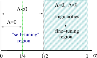
Figure 1: In this figure we illustrate the regions of $\alpha$ where, barring stability issues, “self-tuning” mechanisms can be realised without introduction of singularities. The case with positive bulk cosmological constant is excluded for all values of $\alpha$.

We now follow our discussion in sections 4 and 5 in order to see if there is also in this case a problem with instabilities and, if so, estimate the amount of fine-tuning required.

Taking into account the leading exponential terms for large $y$ using the second or third solution above (51), gives an effective cosmological constant of order

$$\Lambda_{\text{eff}}\sim M_{p}^{4}\,{\rm exp}\left\{-4\,y_{c}\,\sqrt{-\frac{\Lambda\kappa_{5}^{2}}{6}}\right\}$$ (53)

which leads to the requirement

$${\rm exp}\left\{4\,y_{c}\sqrt{-\frac{\Lambda\kappa_{5}^{2}}{6}}\right\}>10^{120}$$ (54)

For the case $\lambda<0$ (second solution in (51)), the stability analysis in section 5 can now be followed, again using the leading contributions at large $y$ for the solution. The requirement to cancel the divergent term coming from (36) gives

$$\tilde{\lambda}^{1/\alpha}\,{\rm exp}\left\{-\frac{2(3-2\alpha)}{2\alpha-1}\,y_{c}\sqrt{-\frac{\Lambda\kappa_{5}^{2}}{6}}\right\}<1$$ (55)

which implies, using (54),

$$\tilde{\lambda}^{1/\alpha}<10^{-\frac{60(3-2\alpha)}{(1-2\alpha)}},$$ (56)

or expressed in terms of an effective cosmological constant

$$\tilde{\lambda}^{\frac{1}{\alpha}}<\left(\frac{\Lambda_{\text{eff}}}{M_{p}^{4}}\right)^{\frac{3-2\alpha}{2(1-2\alpha)}}.$$ (57)

Thus we see that also in this case, strong fine-tuning is needed in order to obtain a stable result.

For the case $\lambda>0$ (third solution in (51)) the argument is modified. Now, the $y$ dependent fluctuations come with the wrong sign

$$S\supset\int d^{4}x\,dy\,\frac{\lambda\alpha\left(1-2\alpha\right)}{2}\,h(y)\left(\frac{d\delta\varphi}{dy}\right)^{2},$$ (58)

with

$$h(y)=\left(\cosh{\left[\sqrt{-\frac{\Lambda\kappa_{5}^{2}}{6}}\,\frac{4\alpha}{1-2\alpha}(|y|+C_{2})\right]}\sqrt{\frac{\lambda(2\alpha-1)\,C_{1}^{2\alpha}}{2\Lambda}}\right)^{\frac{1}{\alpha}}.$$ (59)

This term gives rise to tachyonic KK masses as we see below. There can be positive mass-squared terms from the expansion of the brane Lagrangian. Without fine-tuning they should be of the order of the Planck mass. To analyse the KK spectrum it is useful to redefine the fifth coordinate such that

$$\frac{du}{dy}=\frac{1}{h(y)}.$$ (60)

With this new coordinate we get a free Lagrangian

$$\int_{-y_{c}}^{y_{c}}dy\,h(y)\left(\frac{d\delta\varphi}{dy}\right)^{2}=\int_{-u_{c}}^{u_{c}}du\left(\frac{d\delta\varphi}{du}\right)^{2}.$$ (61)

We periodically continue our set-up beyond the cut-off $u_{c}$. A KK mode (with maximal amplitude on the brane) is,

$$\delta\varphi_{n}=a_{n}\cos\left(M_{n}u\right),$$ (62)

with KK mass

$$M_{n}=\frac{2\pi n}{u_{c}},\,\,\,n\in{\mathbb{Z}}.$$ (63)

If the KK masses were not tachyonic it would be reasonable to truncate the KK tower by a UV cut-off. For tachyonic KK modes one can think of a formally similar mechanism. Tachyonic modes signal an instability. They will stabilise by condensation and result in a different solution to the equations of motion. However, if the wave length of the condensed mode is much shorter than the shortest length characterising our solution one might not notice the difference. In $u$ coordinates, the shortest length appearing in the solution is

$$u\left(y=\infty\right)-u\left(y=y_{c}\right)\sim\frac{1}{M_{P}}\exp\left[-\frac{4\,y_{c}}{1-2\alpha}\sqrt{-\frac{\Lambda\kappa_{5}^{2}}{6}}\right],$$ (64)

where we assumed that all input parameters (except $\lambda$) are of order one in Planck units. Now, consider a mode with wavelength, $u_{c}/n\sim M_{p}^{-1}/n$, given by (64). Integrating over the extra dimension yields

$$\int_{-y_{c}}^{y_{c}}dy\,h(y)\left(\frac{d\delta\varphi_{n}}{dy}\right)^{2}\sim M_{p}\exp\left[\frac{8\,y_{c}}{1-2\alpha}\sqrt{-\frac{\Lambda\kappa_{5}^{2}}{6}}\right]\,a_{n}^{2}.$$ (65)

This tachyonic contribution can be balanced by contributions from expanding the brane Lagrangian. Without fine-tuning such a term will be of order one in Planck units. So, stabilisation of the relevant KK modes is possible if

$$\tilde{\lambda}^{\frac{1}{\alpha}}\exp\left[\frac{8\,y_{c}}{1-2\alpha}\sqrt{\frac{-\Lambda\kappa_{5}^{2}}{6}}\right]<1.$$ (66)

With the estimate for the lower bound on $y_{c}$ (54) we obtain a fine-tuning relation

$$\tilde{\lambda}^{\frac{1}{\alpha}}<10^{-\frac{240}{1-2\alpha}}.$$ (67)

Again we can express this as a function of the effective cosmological constant

$$\tilde{\lambda}^{\frac{1}{\alpha}}<\left(\frac{\Lambda_{\text{eff}}}{M_{p}^{4}}\right)^{\frac{2}{1-2\alpha}}.$$ (68)

8 Relation to Models with Three-Form Potential

In this section we relate our models to dual configurations where the scalar is replaced by a three-form gauge potential $A_{\it 3}$. In particular we see that the model discussed in [13] is dual to the case $\alpha=1/3$, as already observed in [17]. Focusing on the three-form, we consider the following 5d Lagrangian

$$S_{H}=\int d^{5}x\sqrt{-G}\,\frac{\lambda}{2\beta}\left(-\frac{H_{\it 4}^{2}}{4!}\right)^{\beta},$$ (69)

with $H_{\it 4}$ being an exact four-form

$$H_{NOPQ}=\partial_{\left[N\right.}A_{\left.OPQ\right]}.$$ (70)

Numerical factors are chosen for convenience. Instead of considering variations with respect to the three-form $A_{\it 3}$ we can enforce the Bianchi identity with a Lagrange multiplier term

$$S_{\text{LM}}=-\int d^{5}x\,\varphi\,\epsilon^{MNOPQ}\,\partial_{M}H_{NOPQ}$$ (71)

and take variations of the sum, $S_{H}+S_{\text{LM}}$, with respect to the four-form, $H_{\it 4}$, and the Lagrange multiplier, $\varphi$. The resulting equations of motion are

$$\partial_{M}\varphi\,\epsilon^{MNOPQ} =\sqrt{-G}\lambda\left(-\frac{H_{\it 4}^{2}}{4!}\right)^{\beta-1}H^{NOPQ},$$ (72)

$$\partial_{[M}H_{NOPQ]} =0.$$ (73)

The equation obtained by varying $S_{H}$ w.r.t. $A_{\it 3}$ is reproduced as the Bianchi identity, $\partial_{[M}\partial_{N]}\varphi=0$ and (72). To obtain the dual theory we solve the algebraic equation for $H_{\it 4}$ (72) by

$$H^{NOPQ}=\frac{\lambda^{-\frac{1}{2\beta-1}}}{\sqrt{-G}}\left(\partial_{K}\varphi\partial^{K}\varphi\right)^{\frac{1-\beta}{2\beta-1}}\epsilon^{MNOPQ}\partial_{M}\varphi.$$ (74)

Plugging this into the action, $S_{H}+S_{\text{LM}}$ provides the dual action

$$\tilde{S}=\int d^{5}x\sqrt{-G}\left(\frac{1-2\beta}{2\beta}\right)\lambda^{-\frac{1}{2\beta-1}}\left(\partial_{M}\varphi\partial^{M}\varphi\right)^{\frac{\beta}{2\beta-1}}.$$ (75)

In particular we see that the model in [13] is dual to our model with $\alpha=1/3$ and a bulk cosmological constant. In fact, the solution in [13] corresponds precisely to our third solution in the previous section with $\alpha=1/3$, negative bulk cosmological constant and $\lambda(2\alpha-1)<0$. Therefore the instability problem we have discussed above, has to be addressed in this self-tuning proposal as well, as already observed in [18]. With the results presented here this would then lead to a system with a positive cosmological constant, subject to a fine-tuning to be consistent with observations.

9 Conclusions

The possibility that the cosmological constant can be set to (almost) zero by means of extra dimensions, is definitely a very attractive idea. However, so far, all known self-tuning mechanisms of the cosmological constant in extra dimensions have been shown to require hidden fine-tunings, once closer analysis of the mechanism is performed. In the present paper we have discussed a self-tuning mechanism in five dimensions, which makes use of non standard kinetic terms for the self-tuning fields.

Starting with a (complex or real) scalar field with an unorthodox Lagrangian in five dimensions, we have shown that apparently consistent self-tuning solutions arise naturally, which can compensate and cancel the (classical part of the) 4d cosmological constant. A closer look revealed, unfortunately, that fluctuations around the self-tuning solution destabilise the mechanism, unless severe fine-tuning is reintroduced to obtain a small cosmological constant. Addition of a bulk cosmological constant does not improve the situation and the instability, or fine-tuning, persists, as we have shown.

Quite surprisingly, the conditions on our coupling $\lambda$ look very model dependent (on $\alpha$ and a bulk cosmological constant). Here, however we should notice that these are estimates. An accurate treatment should follow the discussion in section 6. Further, the condition on the smallness is not yet a fine-tuning condition. Fine-tuning means that bare quantities have to be chosen very precisely to cancel quantum corrections. The amount of fine-tuning is thus related to the cut-off dependence of quantum corrections. It might happen that taking into account anomalous dimensions of $\lambda$ results finally in a universal fine-tuning condition of the same amount as in the original cosmological constant problem.

Using our analysis, we have also demonstrated that the apparent self-tuning mechanism proposed in [13] is a particular case of our general class of models. This can be easily understood from the fact that the model in [13] uses a three-form potential, which is dual to a scalar field in five dimensions. Thus we have seen that so far a model with a fully consistent self-tuning mechanism (without a hidden fine-tuning) does not exist yet in five dimensions. We expect that similar type of problems might arise in higher dimensions.

References

- [1] S. Weinberg, Rev. Mod. Phys. 61 (1989) 1.
- [2] E. Witten, arXiv:hep-ph/0002297.
- [3] P. Binetruy, Int. J. Theor. Phys. 39 (2000) 1859 [arXiv:hep-ph/0005037].
- [4] U. Ellwanger, arXiv:hep-ph/0203252.
- [5] L. Randall and R. Sundrum, Phys. Rev. Lett. 83, 3370 (1999) [arXiv:hep-ph/9905221].
- [6] L. Randall and R. Sundrum, Phys. Rev. Lett. 83, 4690 (1999) [arXiv:hep-th/9906064].
- [7] O. DeWolfe, D. Z. Freedman, S. S. Gubser and A. Karch, Phys. Rev. D 62, 046008 (2000) [arXiv:hep-th/9909134].
- [8] S. Kachru, M. B. Schulz and E. Silverstein, Phys. Rev. D 62, 045021 (2000) [arXiv:hep-th/0001206].
- [9] N. Arkani-Hamed, S. Dimopoulos, N. Kaloper and R. Sundrum, Phys. Lett. B 480, 193 (2000) [arXiv:hep-th/0001197].
- [10] S. Förste, Z. Lalak, S. Lavignac and H. P. Nilles, Phys. Lett. B 481, 360 (2000) [arXiv:hep-th/0002164].
- [11] S. Förste, Z. Lalak, S. Lavignac and H. P. Nilles, JHEP 0009, 034 (2000) [arXiv:hep-th/0006139].
- [12] C. Csaki, J. Erlich, C. Grojean and T. J. Hollowood, Nucl. Phys. B 584, 359 (2000) [arXiv:hep-th/0004133].
- [13] J. E. Kim, B. Kyae and H. M. Lee, Nucl. Phys. B 613 (2001) 306 [arXiv:hep-th/0101027].
- [14] J. E. Kim, J. Phys. Conf. Ser. 259, 012005 (2010) [arXiv:1009.5071 [hep-th]].
- [15] I. Antoniadis, S. Cotsakis and I. Klaoudatou, arXiv:1005.3221 [hep-th].
- [16] I. Antoniadis, S. Cotsakis and I. Klaoudatou, Class. Quant. Grav. 27, 235018 (2010) [arXiv:1010.6175 [gr-qc]].
- [17] K. S. Choi, J. E. Kim and H. M. Lee, J. Korean Phys. Soc. 40 (2002) 207 [arXiv:hep-th/0201055].
- [18] A. J. M. Medved, J. Phys. G 28 (2002) 1169 [arXiv:hep-th/0109180].
- [19] J. W. Chen, M. A. Luty and E. Ponton, JHEP 0009 (2000) 012 [arXiv:hep-th/0003067].
- [20] S. M. Carroll and M. M. Guica, arXiv:hep-th/0302067.
- [21] I. Navarro, JCAP 0309 (2003) 004 [arXiv:hep-th/0302129].
- [22] Y. Aghababaie, C. P. Burgess, S. L. Parameswaran and F. Quevedo, Nucl. Phys. B 680 (2004) 389 [arXiv:hep-th/0304256].
- [23] Y. Aghababaie et al., JHEP 0309 (2003) 037 [arXiv:hep-th/0308064].
- [24] H. P. Nilles, A. Papazoglou and G. Tasinato, Nucl. Phys. B 677, 405 (2004) [arXiv:hep-th/0309042].
- [25] H. M. Lee, Phys. Lett. B 587 (2004) 117 [arXiv:hep-th/0309050].
- [26] J. Garriga and M. Porrati, JHEP 0408 (2004) 028 [arXiv:hep-th/0406158].
- [27] C. P. Burgess, F. Quevedo, G. Tasinato and I. Zavala, JHEP 0411 (2004) 069 [arXiv:hep-th/0408109].
- [28] C. Wetterich, Phys. Rev. D 81 (2010) 103508 [arXiv:1003.3809 [hep-th]].