version 22.1.2014

Lepton bound states in a fundamental
description of elementary forces

H.P. Morsch

HOFF, Brockmüllerstr. 11, D-52428 Jülich, Germany

E-mail: h.p.morsch@gmx.de

Abstract

In the flavour dependence hadrons and leptons show a mass relation, not expected in the Standard Model. This can be understood in an analysis, based on a particle Lagrangian with Maxwell term, boson-boson coupling and massless fermions (quantons), in which hadrons are described as stationary systems of quantons bound by an electric interaction, whereas leptons represent systems bound magnetically.

PACS/ keywords: 11.15.-q, 12.10.-g, 14.60.-z/ Hadron-lepton relation in the flavour dependence, well understood in a theory based on a Lagrangian with Maxwell term, boson-boson coupling and massless elementary fermions (quantons). Composite systems bound by electric and magnetic forces.

During the last decades our knowledge of the features of fundamental forces has increased largely due to strongly improved detector technologies, accelerators with higher energetic beams and better telescopes and new technologies in astrophysics. However, in the theoretical understanding the Standard Model of particle physics [2] (SM), established 40 years ago, still represents the state of our knowledge. It is a heuristic model constructed from first order gauge theories, different for each fundamental force (but gravitation could not be integrated in the SM). Starting from quantum electrodynamics (QED), each additional force requires a different Lagrangian with additional fields. Further, defaults in these theories to describe the flavour degree of freedom and fermion masses require still more fields. Mass has been explained by the Higgs-mechanism, but neutrino masses need also the postulation of heavy Majorana neutrinos. In total, this indicates clearly that the SM (which has many parameters, which cannot be determined within the model) is far from a fundamental theory of elementary forces, which should have no free parameters. In addition, a fundamental theory should have very few elementary fields, since close to the origin nature is expected to develop only from fields, which are present in the vacuum or can be generated out of it. Experimental evidence for the additional fields needed in the SM have not been found.

Even QED, the best known part of the SM, cannot be regarded as a fundamental theory, since the coupling constant $\alpha_{QED}\sim$1/137 is not understood from first principles. However, the precise prediction of spin properties suggests that QED is close to a fundamental theory. Only the divergencies at $r\to 0$ and $\infty$ appear to be in conflict with nature, which is known to develop in a smooth and finite way. Because of this, a fundamental theory is expected to have a more complex structure than the first order gauge theories in the SM.

A severe problem in the SM is the non-symmetry of hadrons and leptons. Hadrons are assumed to be complex particles composed of elementary fermions (quarks) bound by the strong interaction, whereas leptons are themselves considered as elementary fermions, which couple only by the weak interaction. However, in the flavour dependence of hadron and lepton masses in fig. 1 a relation may be seen (for increasing flavour number hadron and charged lepton masses approach each other), which could reveal that these particles are not completely independent. This is expected, since on a rather fundamental level hadrons and leptons should have a similar origin.

Quite recently a second order extension of QED has been studied [3, 4], which has been found to show all features expected of the long-sought fundamental theory. It is finite and capable to describe systems bound by different forces. Further, with massless elementary bosons and fermions (quantons) this model shows a coupling to the vacuum with average boson and fermion energies $E_{vac}=0$, and very important, it has no free parameters. Applied to the binding of light atoms [5], the self-consistently deduced coupling constant $\alpha$ is consistent with $\alpha_{QED}$, thus leading to an understanding of the fine structure constant. The flavour degree is contained in a discrete ambiguity of the radial extent of bound state solutions, the sum of which is constrained by a vacuum potential sum rule, see ref. [5].

It has to be mentioned that in the past different Lagrangians have been studied with the conclusion that higher order theories should be generally discarded, because they lead to unphysical solutions [7]. However, the important difference to the higher order theories discussed in ref. [7] is that in the present formalism the Lagrangian is gauge invariant and non-physical solutions can be eliminated by strict geometric, mass-radius and energy-momentum relations.

The Lagrangian has been used in the form

$${\cal L}=\frac{1}{\tilde{m}^{2}}\bar{\Psi}\ i\gamma_{\mu}D^{\mu}D_{\nu}D^{\nu}\Psi\ -\ \frac{1}{4}F_{\mu\nu}F^{\mu\nu}~{},$$ (1)

where $\tilde{m}$ is a mass parameter and $\Psi$ a two-component massless fermion field, $\Psi=(\Psi^{+},\Psi^{o})$ and $\bar{\Psi}=(\Psi^{-},\bar{\Psi}^{o})$, with charge and neutral part. Vector boson fields $A_{\mu}$ with coupling $g$ to fermions are contained in the covariant derivatives $D_{\mu}=\partial_{\mu}-i{g}A_{\mu}$. The second term of the Lagrangian represents the Maxwell term with Abelian field strength tensors $F^{\mu\nu}$ given by $F^{\mu\nu}=\partial^{\mu}A^{\nu}-\partial^{\nu}A^{\mu}$, which gives rise to both electic and magnetic effects.

By inserting $D^{\mu}=\partial^{\mu}-i{g}A^{\mu}$ and $D_{\nu}D^{\nu}=\partial_{\nu}\partial^{\nu}-ig(A_{\nu}\partial^{\nu}+\partial_{\nu}A^{\nu})-g^{2}A_{\nu}A^{\nu}$ in eq. (1), the first term of ${\cal L}$ gives rise to a number of different terms, which contain boson and fermion fields and/or their derivatives, see ref. [4]. All terms, which contain the derivative of the fermion field $\partial^{\nu}\Psi$, are related to a rather complex dynamics of the system. For stationary solutions, of only interest here, only two terms of the Lagrangian contribute

$${\cal L}_{2g}=\frac{-ig^{2}}{\tilde{m}^{2}}\ \bar{\Psi}\gamma_{\mu}[A^{\mu}\partial_{\nu}A^{\nu}]~{}\Psi\$$ (2)

and

$${\cal L}_{3g}=\frac{-g^{3}\ }{\tilde{m}^{2}}\ \bar{\Psi}\gamma_{\mu}[A^{\mu}A_{\nu}A^{\nu}]~{}\Psi\ .$$ (3)

The gauge condition $\partial_{\mu}A^{\mu}=0$ used for first order Lagrangians is replaced in the present case by $\partial(\partial_{\nu}A^{\nu})=0$.

Because of its high complexity a general study of the properties of the Lagrangian (1) appears to be rather difficult. So far only fermion matrix elements from the Lagrangians (2) and (3) have been evaluated (derived from generalised Feynman diagrams, see e.g. ref. [8]). However, this has been found to be an efficient and reliable method to generate bound state potentials from the Lagrangian. These matrix elements have been used in the form ${\cal M}=<g.s.|~{}K(\tilde{p}^{\prime}-\tilde{p})~{}|g.s.>\sim\bar{\psi}(\tilde{p}^{\prime})\ K(\tilde{p}^{\prime}-\tilde{p})~{}\psi(\tilde{p})$, where $\psi(\tilde{p})$ is a fermion wave function $\psi(\tilde{p})=\frac{1}{\tilde{m}^{3/2}}\Psi(p)\Psi(k)$ and $K(q)$ a kernel given by $K(q)=\frac{1}{\tilde{m}^{2(n+1)}}\ [O^{n}(q)\ O^{n}(q)]$, were n is the number of derivatives and/or boson fields. For the above Lagrangians (2) and (3) n=3 and $O^{3}(q)=\gamma_{\mu}A^{\mu}\partial_{\nu}A^{\nu}$ and $\gamma_{\mu}A^{\mu}A_{\nu}A^{\nu}$, respectively. This leads to

$${\cal M}_{2g}=\frac{\alpha^{2}}{\tilde{m}^{8}}\bar{\psi}(p^{\prime})\gamma_{\mu}A^{\mu}(q)~{}(\partial_{\nu}A^{\nu}(q))(\partial_{\sigma}A^{\sigma}(q))~{}\gamma_{\rho}A^{\rho}(q)\psi(p)\$$ (4)

and

$${\cal M}_{3g}=\frac{-{\alpha}^{3}}{\tilde{m}^{8}}~{}\bar{\psi}(p^{\prime})\gamma_{\mu}A^{\mu}(q)~{}A_{\nu}(q)A^{\nu}(q)~{}A_{\sigma}(q)A^{\sigma}(q)~{}\gamma_{\rho}A^{\rho}(q)\psi(p)\ ,$$ (5)

where $\alpha=g^{2}/4\pi$.

Before these matrix elements are discussed in detail, one may examine the properties of a simpler (first order) Lagrangian of the form ${\cal L}_{f.o.}=\bar{\Psi}\ i\gamma_{\mu}D^{\mu}\Psi\ -\ \frac{1}{4}F_{\mu\nu}F^{\mu\nu}$. This Lagrangian leads only to one matrix element ${\cal M}_{f.o.}=\frac{-{\alpha}}{\tilde{m}^{4}}~{}\bar{\psi}(p^{\prime})\gamma_{\mu}A^{\mu}(q)~{}\gamma_{\rho}A^{\rho}(q)\psi(p)$. By adding a matrix element with interchanged $\mu$ and $\rho$ (using $\frac{1}{2}(\gamma_{\mu}\gamma_{\rho}+\gamma_{\rho}\gamma_{\mu})=g_{\mu\rho}$) the $\gamma$-matrices can be removed. Further, by an equal time requirement of the two boson fields the matrix element can be written in the form ${\cal M}^{f}_{fo}=\bar{\psi}(p^{\prime})~{}V_{v}(q)~{}\psi(p)$, where $V_{v}(q)$ can be interpreted as boson-exchange interaction of vector structure $V_{v}(q)=\frac{-{\alpha}}{\tilde{m}^{4}}A_{\mu}(q)A^{\rho}(q)$. Since the two boson fields are relativistic, they overlap only momentarily and should not form a stable bound state potential $V_{v}(q)$. Therefore, the existence of a boson-exchange potential in form of the Coulomb potential $V_{coul}(r)=\alpha(\hbar c)~{}1/r$ between two relativistic particles with distance $r$ is not well understood (a non-relativistic approximation for the interaction of relativistic particles, like electrons and protons, is not justified a priori). If the charged particles are in motion with a velocity v relative to the potential, also magnetic effects occur. This leads to the Ampere force law $F_{m}(r)=\frac{\mu_{o}(\hbar c)}{2\pi}I^{2}/r$. Using $I=q\frac{v}{c}c$ and the Maxwell relation $\epsilon_{o}\mu_{o}c^{2}=1$, the Ampere potential $V_{m}(r)=\alpha(\hbar c)~{}(\frac{v}{c})^{2}/r$ is obtained, which has a structure similar to the Coulomb potential, but multiplied with a factor $(\frac{v}{c})^{2}$. Stationary particle states bound in such a potential have never been seriously considered.

Now possible bound state potentials for the second order Lagrangian (1) are discussed by inspecting the structure of the matrix elements ${\cal M}_{2g}$ and ${\cal M}_{3g}$. Again the $\gamma$-matrices can be removed by adding a matrix element with interchanged $\mu$ and $\rho$. Further, the derivatives of boson fields in ${\cal M}_{2g}$ may be written in the form $(\partial_{\nu}A^{\nu}(q))(\partial_{\sigma}A^{\sigma}(q))=\frac{1}{2}\partial_{\nu}[\partial_{\sigma}(A_{\mu}A^{\mu})^{\sigma}]^{\nu}$, using the above gauge condition. In addition, the two boson fields on the right and left of eq. (5) can be combined (analogue to the fermion wave functions) to (quasi) wave functions $W_{\mu}^{\nu}(q)=\frac{1}{\tilde{m}}A_{\mu}(q)A^{\nu}(q)$, whereas the remaining two boson fields may be understood as a boson-exchange interaction of vector structure $V_{\mu}^{\nu}(q)\sim W_{\mu}^{\nu}(q)$ ($\mu\neq\nu$) similar to that of first order theory discussed above. The fact that two boson fields can be combined to wave functions leads quite naturally to a finite theory, in which the wave functions are normalised.

Similar to the first order case, non-vanishing matrix elements can be obtained only, if there is spacial overlap of the boson fields at a given time. However, the important difference to the first order case is that in addition to the boson-exchange matrix element ${\cal M}_{3g}$ a second term of derivative structure ${\cal M}_{2g}$ exists, which leads to a dynamical stabilisation of the system. If a $q\bar{q}$ pair is created momentarily, this term leads to confinement, since the corresponding binding energy is positive. Consequently, the created fermion pair is locked in a bound state. The equal time requirement gives rise to a reduction of the fermion four-vectors to three-vectors in momentum or r-space, while the boson vectors are reduced to two dimensions. The boson wave functions $W_{\mu}^{\nu}(q)$ give scalar and vector components $w_{s}(q)$ and $w_{v}(q)$, whereas $V_{\mu}^{\nu}(q)$ yields an interaction potential $v_{v}(q)\sim w_{v}(q)$. In this way, the fermion matrix elements (4) and (5) can be written by

$${\cal M}^{f}_{2g}=\frac{\alpha^{2}}{2\tilde{m}^{6}}\bar{\psi}(p^{\prime})\ w_{s,v}(q)\partial^{2}w_{s,v}(q)\ \psi(p)\ ,$$ (6)

and

$${\cal M}^{f}_{3g}=\frac{-{\alpha}^{3}}{\tilde{m}^{5}}~{}\bar{\psi}(p^{\prime})w_{s,v}(q)~{}v_{v}(q)~{}w_{s,v}(q)\psi(p)\ .$$ (7)

The bosonic part of eq. (7) can also be written in the form of a matrix element, in which the wave functions $w_{s,v}(q)$ are connected by $v_{v}(q)$

$${\cal M}^{g}=\frac{-\alpha^{3}}{\tilde{m}^{2}}\ w_{s,v}(q)v_{v}(q)w_{s,v}(q).$$ (8)

This matrix element shows binding of two bosons in the potential $v_{v}(q)$. According to the virial theorem the term $\partial^{2}w_{s}(q)$ in eq. (6) is related to the kinetic energy of these bosons. In a transformation to r-space the bosonic part of eq. (6) gives rise to a Hamiltonian, which may be written in the form

$$-\frac{\alpha^{2}(\hbar c)^{2}F_{2g}}{4\tilde{m}}~{}\Big{(}\frac{d^{2}w_{s}(r)}{dr^{2}}+\frac{2}{r}\frac{dw_{s}(r)}{dr}\Big{)}+V_{2g}(r)~{}w_{s}(r)=E_{i}~{}w_{s}(r)~{},$$ (9)

where the factor $F_{2g}$ is due to the Fourier transformation of the boson kinetic energy. This leads to a binding potential

$$V_{2g}(r)=\frac{\alpha^{2}(\hbar c)^{2}F_{2g}}{4\tilde{m}}\ \Big{(}\frac{d^{2}w_{s}(r)}{dr^{2}}+\frac{2}{r}\frac{dw_{s}(r)}{dr}\Big{)}\frac{1}{\ w_{s}(r)}+E_{o}\ ,$$ (10)

where $E_{o}$ the energy of the lowest eigenstate. A connection to the vacuum can be made by assuming $E_{o}=\tilde{E}_{vac}=0$. This potential leads to a stabilisation of the system. It can be identified with the confinement potential, required in hadron potential models [9] and shows an almost linear increase towards larger radii.

Writing the matrix element ${\cal M}^{f}_{3g}$ in the form ${\cal M}^{f}_{3g}=\bar{\psi}(p^{\prime})\ V_{3g}(q)\ \psi(p)$, this leads to a three-boson potential

$${V}^{s,v}_{3g}(q)=\frac{-\alpha^{3}}{\tilde{m}^{2}}~{}w_{s,v}^{2}(q)v_{v}(q)\$$ (11)

with the interaction $v_{v}(q)\sim w_{v}(q)$. Fourier transformation to r-space yields a folding potential

$$V^{s,v}_{3g}(r)=-\frac{\alpha^{3}\hbar c}{\tilde{m}}\int dr^{\prime}w_{s,v}^{2}(r^{\prime})\ v_{v}(r-r^{\prime})~{}.$$ (12)

From the general structure of the fermion matrix element in eq. (7) one can see that there are two $q\bar{q}$ states (with quantum numbers $J^{\pi}=1^{-}$) with scalar and vector boson wave functions $w_{s,v}(r)$ and corresponding fermion wave functions $\psi_{s,v}(r)\sim w_{s,v}(r)$. Further, there are two $q\bar{q}$ p-states (with quantum numbers $J^{\pi}=0^{+}$) with similar wave functions, see e.g. ref. [6].

The fermion wave functions have to be orthogonal, leading to the constraint

$$\int r^{2}dr~{}\psi_{s}(r)\psi_{v}(r)=\int r^{2}dr~{}w_{s}(r)w_{v}(r)=<r_{w_{s},w_{v}}>=0\ .$$ (13)

To satisfy this condition, $w_{v}(r)$ may be written in the form of a p-wave function

$$w_{v}(r)=w_{v,o}~{}[w_{s}(r)+\beta R\ \frac{dw_{s}(r)}{dr}]~{},$$ (14)

where $w_{v,o}$ is obtained from the normalisation $2\pi\int rdr\ w_{v}^{2}(r)=1$ and $\beta R$ determined by $\beta R=-\int r^{2}dr~{}w_{s}(r)/\int r^{2}dr~{}[dw_{s}(r)/dr]$. Interestingly, orthogonality gives rise to another quite natural condition for the deepest bound state, requiring that the interaction takes place inside the bound state volume of $w_{s}^{2}(r)$. This leads to

$$|V^{v}_{3g}(r)|\sim{c}\ w^{2}_{s}(r)\ .$$ (15)

The conditions (13)-(15) lead to a boson wave function $w_{s}(r)$, which can be approximated by

$$w_{s}(r)=w_{s,o}\ exp\{-(r/b)^{\kappa}\}\ ,$$ (16)

where $w_{s,o}$ is fixed by the normalisation $2\pi\int rdr\ w_{s}^{2}(r)=1$. The parameters $b$ and $\kappa$ have to be determined by boundary conditions as discussed below. Different flavour states are obtained by solutions with different slope parameter $b$, which are constrained by a vacuum potential sum rule, see e.g. ref. [5]. The interaction $v_{v}(r)$ is given by $v_{v}(r)=\hbar c~{}w_{v}(r)$.

Binding energies have been calculated from the potentials $V_{ng}(r)$ by using the virial theorem in the form $4\pi[\int r^{2}dr~{}\psi^{2}(r)V_{ng}(r)-\frac{1}{2}\int r^{3}dr~{}\psi^{2}(r)\frac{d}{dr}V_{ng}(r)]=E_{f}$, where $\psi(r)$ are fermion wave functions with a form similar to the boson wave functions in eqs. (14) and (16). In addition, eq. (8) shows that $V^{s}_{3g}(r)$ can be interpreted as bound state of bosons. Its binding energy $E_{g}$ has been calculated by the corresponding form $2\pi[\int rdr~{}w_{s}^{2}(r)v_{v}(r)-\frac{1}{2}\int r^{2}dr~{}w_{s}^{2}(r)\frac{d}{dr}v_{v}(r)]=E_{g}$. For massless fermions the mass of the system $M^{s,v}$ is given by the absolute binding energies in $V_{2g}(r)$ and $V^{s,v}_{3g}(r)$, $M^{s,v}=-E^{3g}_{f_{s,v}}+E^{2g}_{f}$, while the reduced mass is given by $\tilde{m}=M^{s}/2$.

In order to make an evaluation of the potentials other constraints are needed, which connect the coupling constant $\alpha$ to the shape parameters and the mass parameter $\tilde{m}$. $(q\bar{q})^{n}$ systems can be bound by an electric interaction. One condition is the energy-momentum relation, important for relativistic bound states. For binding in the potential $V^{s}_{3g}(q)$ the negative fermion and boson binding energies $E_{f}^{s}$ and $E_{g}$ have to be compensated by their root mean square momenta $<q^{2}_{v}>=\int dq~{}q^{3}~{}v(q)/\int dq~{}q~{}v(q)$ in the potentials $V_{3g}(r)$ and $v_{v}(r)$, respectively

$$<q^{2}_{V_{3g}}>+<q^{2}_{v_{v}}>=(E_{f}^{s}+E_{g})^{2}\ .$$ (17)

Another condition can be derived from the confinement potential (10), see ref. [4], which leads to

$$Rat_{conf}=\frac{(\hbar c)^{2}}{\tilde{m}^{2}<r^{2}_{w_{s}}>}=1\ .$$ (18)

By these conditions all parameters are interrelated and can be uniquely determined for a given mass of the system. The above formalism has been discussed for electric binding of quantons in hadronic $q\bar{q}$ systems in ref. [4, 6], further for the description of light atomic systems in ref. [5]. Importantly, for atoms the deduced coupling constant has been found to be consistent with $\alpha_{QED}\sim 1/137$, thus leading to an understanding of this constant from first principles. For the much smaller hadronic $q\bar{q}$ bound states the magnitude of the coupling constant is significantly larger.

Now a new situation is discussed, in which the fermion fields are in relative motion with velocity v to lead to stationary systems, which are bound magnetically. This is not possible for uniform motion of the total density, e.g. as a rotation of a $q\bar{q}$-system (possible for an electrically bound system), but requires a more complex system with at least two fermions, in which the positive and negative fermions move in opposite direction to each other with a relative velocity $({v}/{c})$. This is possible in $(q\bar{q})^{n}q$ systems, requiring that the fermion momenta add up to zero, $\sum_{i=1,n}\vec{<q_{\psi_{i}}>}=0$. Described by fermion densities this leads to $<q^{2}_{V_{3g}}>=0$. Due to the opposite motion of positive and negative fermions, on the average all electric interactions cancel out. With a reduction of the potentials by a factor $({v}/{c})^{2}$ (see the first order case discussed above) this gives rise to an energy-momentum relation

$$<q^{2}_{v_{v}}>({v}/{c})^{2}=(E_{f}^{s}+E_{g})^{2}\ .$$ (19)

Another difference from electric bound states, p-wave states with nodes in the wave functions do not lead to stable magnetic bound states, thus allowing only one stable magnetic state with boson and fermion wave functions $w_{s}(r)$ and $\psi_{s}(r)$. Further, the confinement potential leads to the condition

$$Rat_{conf}=\frac{(\hbar c)^{2}({v}/{c})^{2}}{\tilde{m}^{2}<r^{2}_{w_{s}}>}=1\ .$$ (20)

Finally, $({v}/{c})^{2}$ has to be included in the bound state potential $V_{3g}(r)$. Altogether this gives three conditions, by which $({v}/{c})^{2}$ is determined

$$({v}/{c})^{2}_{conf}=\frac{\tilde{m}^{2}<r_{w_{s}}^{2}>}{(\hbar c)^{2}}\ ,$$ (21)

$$({v}/{c})^{2}_{mom}=(E^{s}_{f}+E_{g})^{2}/<q^{2}_{v_{v}}>\ ,$$ (22)

$$({v}/{c})^{2}_{pot}=(\alpha_{fit}^{3})/\alpha^{3}\ ,$$ (23)

where $\alpha_{fit}^{3}=\alpha^{3}({v}/{c})^{2}$ is the coupling constant in eq. (12) adjusted to get the binding energy $E_{f}^{s}$. Only if the same value of $({v}/{c})^{2}$ is obtained in all three expressions (21)-(23), a stable bound state is created.

The above formalism has been used to describe the structure of charged and neutral leptons $e$, $\mu$, $\tau$ and $\nu_{e}$, $\nu_{\mu}$, $\nu_{\tau}$, which are assumed as stationary $(q\bar{q})^{n}q$ systems bound magnetically. The shape parameter $\kappa$ has been taken from the analysis of hadrons [4], whereas the slope parameter and the coupling constant $\alpha$ has been adjusted to give the same value of $({v}/{c})^{2}$ from all three conditions (21)-(23).

First, neutrino bound states are discussed. Starting from a pure $q^{o}\bar{q}^{o}q^{o}$ structure, magnetic binding without motion of charge is not possible. However, a $q^{o}\bar{q}^{o}$ pair can change to two $(q^{+}q^{-})$ pairs, in which the positive and negative fermions move in opposite direction to each other with relative velocity $v/c$. This can lead to magnetic binding. Indeed, in such an analysis the three boundary conditions (21)-(23) can be fulfilled (which is far from trivial), leading to a system with a very small radius. This is conceivable, since the magnetic force is only strong enough at extremely small distances. First, the slope parameter $b$ has been varied to get the same value of $({v}/{c})^{2}$ from the relations (21) and (22); then $\alpha$ has been adjusted to get the same value of $({v}/{c})^{2}$ from relation (23). This was possible for all three neutrinos and confirms the conjecture that these systems are bound magnetically. The used parameters, masses, deduced mean square radii and values of $({v}/{c})^{2}$ are given in table 1. The masses have been used from ref. [10], which yield mass square differences $m_{\nu_{\mu}}^{2}-m_{\nu_{e}}^{2}=\Delta m^{2}_{sol}$ and $m_{\nu_{\tau}}^{2}-m_{\nu_{e}}^{2}=\Delta m^{2}_{atm}$ consistent with the values $\Delta m^{2}_{sol}\simeq 7.6\ 10^{-5}(eV)^{2}$ and $\Delta m^{2}_{atm}\simeq 2.4\ 10^{-3}(eV)^{2}$ deduced from neutrino oscillation experiments [11].

Results on the shape of the interaction $v_{v}(r)$ is given in the upper part of fig. 2 in comparison to the $1/r$ dependence of the Ampere potential. In the middle part the r-dependence of boson density and potentials $V_{eg}(r)$ are displayed, which shows that relation (15) is well fulfilled. The confinement potential $V_{2g}(r)$ is shown in the lower part, which has a form rather similar to that deduced for hadrons. Although the absolute magnitude is rather low for very small bound states, the positive binding energy in this potential is responsible for stabilisation of the system.

Table 1: Parameters ($b$ in fm) and masses, mean square radii (in fm) and deduced values of $({v}/{c})^{2}$ for the different systems with flavour number $n_{f}$.

$n_{f}$	System	$\kappa$	$b$	$\alpha$	mass	$<r^{2}_{w}>^{1/2}$	$({v}/{c})^{2}$
1	$\nu_{e}$	1.4	7.96 10-9	2.0	0.015 eV	6.8 10-9	6.7 10-38
2	$\nu_{\mu}$	1.4	3.96 10-9	2.0	0.01735 eV	3.4 10-9	2.2 10-38
3	$\nu_{\tau}$	1.4	2.25 10-9	2.0	0.0512 eV	1.9 10-9	6.4 10-38
1	$e$	1.4	3.95 10-10	2.0	0.51 MeV	3.4 10-10	1.9 10-25
2	$\mu$	1.4	2.65 10-10	2.0	105.7 MeV	2.3 10-10	3.7 10-21
3	$\tau$	1.4	1.98 10-10	2.0	1777 MeV	1.7 10-10	5.9 10-19

Table 1 shows indeed very small radii of the order of $10^{-9}$ fm. The extracted value of $\alpha$$\sim$2 may be used to show a qualitative relation between magnetic and electric bound states. For electric binding of $q\bar{q}$ systems rather similar values of $\alpha$ of 1.5 and 2.4 have been extracted for $\Phi$ and $J/\psi$ mesons with a masses of 1.02 and 3.10 GeV, respectively, and mean radii square of 0.15 and 0.016 fm², see ref. [4]. This may indicate that for $\nu_{e}$ the magnetic force gives rise to a bound state energy smaller than the electric force by a factor of about 10^-11 and a radius smaller by a factor of 3 10^-8.

The value of $({v}/{c})^{2}$ of several $10^{-38}$ leads to a total coupling constant $\alpha_{tot}=\alpha^{3}({v}/{c})^{2}$ of the order of 10^-37, which is only two orders of magnitude larger than the gravitational coupling $G_{N}m_{1}m_{2}/\hbar c=6.707~{}10^{-39}$. For composite systems larger radii are expected and the coupling constant should decrease further. This supports the conclusion of a previous less constrained neutrino analysis [10] that gravitation may be due to magnetic interactions of particles in matter. For a real proof of this conjecture calculations have to show that indeed the strict boundary conditions for magnetic bound states are fulfilled for gravitational systems. Preliminary studies [3] show that rotational velocities of galaxies are well described in the present approach (without dark matter contributions). However, it should be verified also that the complex dynamics of the present Lagrangian with a mixing of motion and bound state creation is consistent with astrophysical observations.

For charged leptons a quite similar structure as for neutrinos is expected. Again, for a pure $q^{o}\bar{q}^{o}q^{-}$ configuration no interactions take place. If the $q^{o}\bar{q}^{o}$ pair decays to two $q^{+}q^{-}$ pairs with opposite velocity v of positive and negative fermions, again a magnetic bound state should be formed, for with the conditions (21)-(23) are fulfilled. This is indeed the case, indicating that also charged leptons can be regarded as magnetic bound states, with radii still smaller than of neutrinos. The results are also given in table 1.

For the electron the boson-density and the potentials are given in the upper part of fig. 3, which show that the boundary condition (15) is well fulfilled. Also the Fourier transformed quantities are in good agreement, as shown in the middle part. The shape of the confinement potential $V_{2g}(r)$, displayed in the lower part, is also rather similar as for neutrinos. Importantly, as seen in the upper part of fig. 3, the average radius of several $10^{-10}$ fm is in agreement with results from M$\phi$ller scattering [12], from which the electron radis has been estimated to be $<10^{-9}$ fm.

Further, the magnetic bound state interpretation is in agreement with the anomalous moments of charged leptons. Writing the magnetic moment by $\vec{\mu}_{l}=\frac{e\hbar}{2m_{l}}\sum_{i}\int r^{2}dr\bar{\psi}_{i}(r)\vec{\frac{s}{\hbar}}\psi_{i}(r)$, the fact that two fermion densities are involved yields $\vec{\mu}_{l}=2~{}\frac{e\hbar}{2m_{l}}$. This is consistent with the $e$ and $\mu$ data, apart from a 1 ${}^{o}/_{oo}$ effect due to higher order mass corrections [13].

Table 2: Comparison of mass ratio squares $F_{m}^{2}$, mean radius squares $F_{rad}^{2}$ and resulting values of $({v}/{c})^{2}$ for charged leptons in comparison with the results in table 1 for the three different charged/neutral lepton pairs.

$n_{f}$	System	$F_{m}^{2}$	$F_{rad}^{2}$	$F_{m}^{2}F_{rad}^{2}({v}/{c})_{\nu}^{2}$	$({v}/{c})_{c}^{2}$
1	e, $\nu_{e}$	1.16 1015	2.5 10-3	1.9 10-25	1.9 10-25
2	$\mu,\nu_{\mu}$	3.71 1019	4.6 10-3	3.7 10-21	3.7 10-21
3	$\tau,\nu_{\tau}$	1.21 1021	8.0 10-3	6.2 10-19	5.9 10-19

It is interesting to compare the flavour dependence of electric and magnetic bound states. Whereas for electric $q\bar{q}$ bound states $\alpha^{3}$ increases as a fuction of $n_{f}$, see ref. [4], for magnetic bound states the product $\alpha^{3}({v}/{c})^{2}$ should change. The results in table 1 show that only $({v}/{c})^{2}$ changes, whereas $\alpha$ stays constant.

This independence on $\alpha$ for magnetic bound states allows to describe the different masses and corresponding $({v}/{c})^{2}$ values by a simple mass-radius relation. First, the relative velocity square of a charged lepton $({v}/{c})^{2}_{c}$ may be proportional to that of the corresponding neutrino multiplied with the square of the ratio of their masses $F_{m}^{2}=(m_{c}/m_{\nu})^{2}$. This cannot be entirely correct, because both the masses and radii of the systems change. Taking both mass ratio and $F_{rad}^{2}=<r^{2}_{c}>$/$<r^{2}_{\nu}>$ into account yields

$$({v}/{c})_{c}^{2}\simeq F_{m}^{2}F_{rad}^{2}({v}/{c})_{\nu}^{2}\ .$$ (24)

In table 2 the different ratios and products are given for the three flavour charged/neutral lepton pairs. This shows that the differences of the extracted velocities of charged and neutral leptons in table 1 are well described by the simple relation (24). By this, the different mass dependences of charged and neutral leptons in fig. 1 are well understood, arising from orthogonality of the wave functions of the different flavour states. Also it should be stressed that the good agreement between charged and neutral leptons has been achieved by using the neutrino masses from the ref. [10]. This supports the correctness of the extracted neutrino masses.

Finally it is important to mention that due to the $(q\bar{q})^{n}q$ structure of leptons mesons of $(q\bar{q})^{n}$ structure can decay only to lepton-antilepton pairs, whereas baryons of $(q\bar{q})^{n}q$ structure decay to baryon and lepton-antilepton pairs. These decays are weak due to an extremely small overlap of the very different hadron and lepton wave functions.

In conclusion, a new theoretical framework for the description of fundamental forces has been discussed, based on a generalisation of electromagnetic interactions. Compared to the SM, in which an understanding of the mass of different flavour states of hadrons and leptons requires supersymmetric fields, but also Higgs-field and Majorana neutrinos, in the present formalism none of these fields are needed.

With massless elementary fermions (quantons) and massless gauge bosons, a direct coupling to the absolute vacuum with average energy $\tilde{E}_{vac}=0$ is obtained; further, severe boundary conditions for electric and magnetic bound states are fulfilled, by which all parameters of the model are determined. This shows that all criteria of a fundamental theory of relativistic particle bound states are fulfilled, which leads most likely to a coherent description of all fundamental forces of nature. For more extended studies it could be advantageous, if other solutions of the Lagrangian (1) would be found, which go beyond the presently used evaluation of matrix elements.

Only a minimum of elementary fields is needed, one boson gauge field and charged and neutral fermion (quanton) fields (of electric and magnetic structure). Together with the fact that hadrons are understood as electric and leptons by magnetic bound states, this emphasizes the inherent symmetry of electic and magnet phenomena of Maxwell’s theory also in fundamental physics.

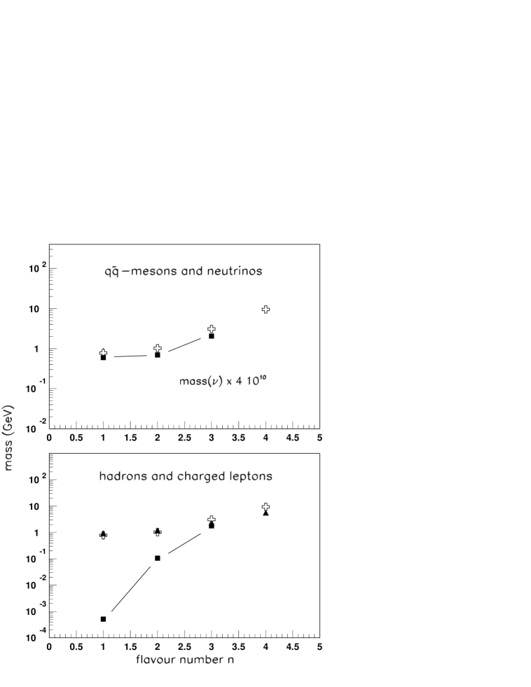
Figure 1: Flavour dependence of hadron and lepton masses. Upper part: $q\bar{q}$ meson masses (open crosses) as a function of the flavour number $f_{n}$=1-4 ($\omega$, $\Phi$, $J/\psi$ and $\Upsilon$) and masses of neutral leptons taken from ref. [10] ($f_{n}$=1-3 relate to $\nu_{e}$, $\nu_{\mu}$ and $\nu_{\tau}$), given by solid squares. Lower part: Similar plot for baryons (triangles), $q\bar{q}$ mesons (open crosses) and charged leptons (solid squares). For baryons $f_{n}$=1-4 represent nucleon, $(\Lambda,\Sigma)$, $\Lambda_{c}$ and $\Lambda_{b}$, for leptons $f_{n}$=1-3 correspond to $e$, $\mu$ and $\tau$. The straight lines are to guide the eye.

Figure 2: Self-consistent solution for the $\nu_{e}$ system. Upper part: Relative interaction $v_{v}(r)$ in comparison with the Ampere potential $(\sim 1/r)$ given by dot-dashed line. Middle part: Boson density $w_{s}^{2}(r)$ (dot-dashed line) and boson-exchange potentials $|V^{s,v}_{3g}(r)|$ given by dashed and solid lines, respectively. Lower part: Deduced confinement potential $V_{2g}(r)$.

Figure 3: Self-consistent solution for the electron system. Upper part: Boson density $w_{s}^{2}(r)$ (dot-dashed line) and boson-exchange potentials $|V^{s,v}_{3g}(r)|$ given by dashed and solid lines, respectively. Middle part: Fourier transformed boson density $w_{s}^{2}(q)$ (dot-dashed line) and boson-exchange potential $|V^{v}_{3g}(q)|$ given by solid line. Lower part: Deduced confinement potential $V_{2g}(r)$.

References

- [1]
-
[2]
Review of particle properties, K. Nakamura et al.,
J. Phys. G 37, 075021 (2010);
http://pdg.lbl.gov/ and refs. therein - [3] H.P. Morsch, EPJ Web of Conferences 28, 12068 (2012), Hadron Collider Physics Symposium, Paris 2011 (open access)
- [4] H.P. Morsch, Universal Journal of Physics and App. 1, 252 (2013), arXiv 1112.6345 [gen-ph]
- [5] H.P. Morsch, arXiv 1104.2574 [hep-ph]
- [6] H.P. Morsch, arXiv 1210.0244 [gen-ph]
- [7] J.Z. Simon, Phys. Rev. D 41, 3720 (1990); A. Foussats, E. Manavella, C. Repetto, O.P. Zandron, and O.S. Zandron, Int. J. theor. Phys. 34, 1 (1995); V.V. Nesterenko, J. Phys. A: Math. Gen. 22, 1673 (1989); and refs. therein
- [8] see e.g. I.J.R. Aitchison and A.J.G. Hey, “Gauge theories in particle physics”, Adam Hilger Ltd, Bristol, 1982; or M.E. Peskin and D.V. Schroeder, “An introduction to quantum field theory”, Addison-Wesley Publ. 1995
- [9] R. Barbieri, R. Kögerler, Z. Kunszt, and R. Gatto, Nucl. Phys. B 105, 125 (1976); E. Eichten, K.Gottfried, T. Kinoshita, K.D. Lane, and T.M. Yan, Phys. Rev. D 17, 3090 (1978); S. Godfrey and N. Isgur, Phys. Rev. D 32, 189 (1985); D. Ebert, R.N. Faustov, and V.O. Galkin, Phys. Rev. D 67, 014027 (2003); and refs. therein
- [10] H.P. Morsch, arXiv 1104.2576 [hep-ph], v1
-
[11]
T. Schwetz, M. Tortola, and J.W.F.Valle, New
J. Phys. 10, 113011 (2008);
K. Nakamura and S.T. Petcov, JPG 37, 37 (2010) and refs. therein - [12] Mller scattering, see www.electronformfactor.com
- [13] J. Schwinger, Phys. Rev. 73, 416 (1948)