Quantum Percolation Transition from Graphene to Graphane:
Graph Theoretical Approach

Abstract

Graphane is obtained by perfectly hydrogenating graphene. There exists an intermediate material, partially hydrogenated graphene (which we call hydrographene), interpolating from pure graphene to pure graphane. It has various intriguing electronic and magnetic properties. We investigate a metal-insulator transition, employing a quantum-site percolation model together with a graph theoretical approach. Hydrographene is an exceptional case in which electronic properties cannot be determined solely by the density of states at the Fermi energy. Though there are plenty of zero energy state in wide range of hydrogenation density, most of them are insulating states. We also demonstrate that it shows a bulk ferromagnetic property based on the Lieb theory.

Graphene is one of the main topics in condensed matter physics because of its unusual electronic propertiesGraphEx ; NetoRev . It is a promising material to design future nanoelectronic devices. To make a device it is necessary to confine electrons within a certain finite domain. However, this is impossible in a graphene sheet by applying electric field due to the Klein tunneling effect, which is an intrinsic nature of Dirac electrons. One method is to cut graphene to form a required domain. Resultant graphene derivatives such as graphene nanoribbonsRibbon and graphene nanodisksDisk show remarkable electronic and magnetic properties.

Recently graphane has been attracting much attentionSofo ; Elias ; Balog ; Savche . It is a graphene derivative obtained by perfectly hydrogenating graphene (Fig.1). Graphene is a semimetal with each carbon forming an sp² orbital, while graphane is an insulator with each carbon forming an sp³ orbital. Graphane provides us with an alternative method of confining electrons within a finite domain, since $\pi$-electrons are excluded from hydrogenated carbons. Namely, by dehydrogenating a finite region of a graphane sheet, electron can be confined within this region. By dehydrogenating a graphane sheet according to a circuit pattern, in principle it is possible to fabricate a graphene-graphane complex, embodying various electronic functionsNovPhys .

In this paper, we explore an intermediate material, partially hydrogenated graphene, which interpolates from pure graphene to pure graphaneBalog . Let us call it hydrographene. There are two types of hydrogenation, single-sided percolation and double-sided percolation. Employing a graph theoretical approach to the site-percolation modelPercoBook , we present an intuitive and physical picture revealing the electronic and magnetic properties of hydrographene with hydrogenation density $q$, $0\leq q\leq 1$. As $q$ increases, there occurs a metal-insulator transition at $q_{\text{c}}$. It is mapped to a ferromagnet-paramagnet transition in a Potts model with $q_{\text{c}}$ corresponding to a critical temperature $T_{\text{c}}$. We remark that hydrographene is an exceptional case in which electronic properties cannot be determined solely by the density of states (DOS) at the Fermi energy. This is because there emerge a number of insulating states which contribute to the DOS at the Fermi energy but not to the conductivity. We also show that it is a bulk ferromagnet in the context of the Lieb theory. We find that single-sided hydrogenation is more efficient to form large magnetic moment than double-sided hydrogenation.

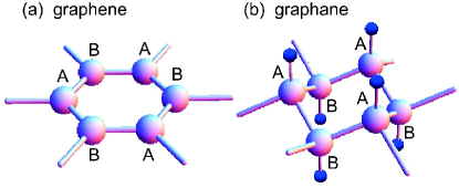
Figure 1: (Color online) (a) Illustration of graphene. There are carbons on a honeycomb lattice. They are grouped in two inequivalent sites A and B. (b) Illustration of graphane. Hydrogens are attached upwardly to A sites, and downwardly to B sites. A honeycomb lattice is distorted.

Model: In hydrographene a finite density of hydrogens are absorbed randomly to grapheneBalog . Carbons with absorbed hydrogen form an sp³ bond, where no $\pi$-electron exists. To simulate this fact we model the system by the Hamiltonian,

$$H=\sum_{\left\langle i,j\right\rangle}tc_{i}^{\dagger}c_{j}+V{\sum_{r}}^{\prime}c_{r}^{\dagger}c_{r},$$ (1)

where $c_{j}$ ($c_{i}^{\dagger}$) is the annihilation (creation) operator of $\pi$-electron, $t=2.7$ [eV] is the transfer energy, and $\left\langle i,j\right\rangle$ denotes the next-nearest neighbor sites of the honeycomb lattice. To exclude the electron at the hydrogenated site $r$ we have imposed an infinitely large on-site potential $V$ at $r$. Thus the sum ${\sum_{r}^{\prime}}$ runs over the lattice sites where carbons are hydrogenated.

We analyze a quantum site-percolation problem based on this Hamiltonian. Electromagnetic properties depend on percolation networks (Fig.2), where hydrogenated carbons have been removed from the network. The resultant carbon network is nothing but a graph with vertices corresponding to carbons. The model Hamiltonian has one-to-one correspondence to the adjacency matrix of a graph. Though the Hamiltonian is noninteracting, the problem is highly nontrivial because percolation network is highly nontrivial.

Graphene is a bipartite system made of carbons at two inequivalent sites (A and B sites) on a honeycomb lattice, as illustrated in Fig.1(a). These carbons can absorb hydrogens randomly. The reaction with hydrogen is reversible, so that the original metallic state and the lattice spacing can be restored by annealingElias . However, the way of attachment is opposite between the A and B sites in graphane [Fig.1(b)]. As a matter of convenience, hydrogens are absorbed upwardly to A sites and downwardly to B sites. We can investigate two types of percolation problems in hydrographene. In one case, hydrogenation occurs randomly on both A and B sites. We call it double-sided percolation. In the other case, hydrogenation occurs only on A sites. We call it single-sided percolation. Single-sided hydrogenation can be manufactured by resting graphene on a Silica surfaceElias .

The number of lattice sites with no defects is $N_{\text{c}}$. We assume $N_{\text{c}}$ is even for simplicity. We define the hydrogenation density by $q=M/N_{\text{c}}$ for double-sided hydrogenation and $q=2M/N_{\text{c}}$ for single-sided hydrogenation, where $M$ is the number of hydrogenated carbons, $M={\sum_{r}^{\prime}}$. We choose the positions of hydrogenated carbons by the Monte Carlo method. Physical quantities are to be determined by taking the statistical average.

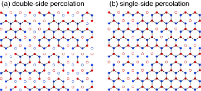
Figure 2: (Color online) Graph representation of percolation network in a honeycomb lattice. (a) 30% hydrogenation on the two sides. The system is not connected. (b) 30% hydrogenation on one side. The system is connected.

Isolated carbons: We refer to carbons with no adjacent carbons as isolated carbons, to those with one adjacent carbon as edge carbons, to those with two adjacent carbons as corner carbons, and to those with three adjacent carbons as bulk carbons. We apply a combinatorial theory and estimate the numbers of these different types of carbons by using the fact that each site is occupied with probability $q$. We also use the quantity $p=1-q$ in what follows.

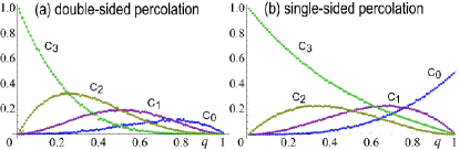
Figure 3: (Color online) The numbers of isolated carbons $C_{3}$, edge carbons $C_{2}$, corner carbons $C_{1}$ and bulk carbons $C_{0}$ in unit of $N_{\text{c}}$. The horizontal axis is the hydrogenation density $q$.

In the case of double-sided percolation, we calculate the number of isolated carbons to be $C_{0}=pq^{3}N_{\text{c}}$, that of edge carbons to be $C_{1}=3p^{2}q^{2}N_{\text{c}}$, that of corner carbons to be $C_{2}=3p^{3}qN_{\text{c}}$ and that of bulk carbons to be $C_{3}=p^{4}N_{\text{c}}$. They satisfy the relation $C_{0}+C_{1}+C_{2}+C_{3}=pN_{\text{c}}$. The total bond number is $\frac{1}{2}\left(C_{1}+2C_{2}+3C_{3}\right)=\frac{3}{2}p^{2}N_{\text{c}}$.

In the case of single-sided percolation, we calculate the number of isolated carbons to be $C_{0}=\frac{1}{2}q^{3}N_{\text{c}}$, that of edge carbons to be $C_{1}=\frac{3}{2}pq^{2}N_{\text{c}}$, that of corner carbons to be $C_{2}=\frac{3}{2}p^{2}qN_{\text{c}}$ and that of bulk carbons to be $C_{3}=\frac{1}{2}\left(p^{3}+p\right)N_{\text{c}}$. They satisfy the relation $C_{0}+C_{1}+C_{2}+C_{3}=\frac{1}{2}\left(p+1\right)N_{\text{c}}$. The total bond number is $\frac{1}{2}\left(C_{1}+2C_{2}+3C_{3}\right)=3pN_{\text{c}}$.

We show the numbers of various types of carbons estimated in this way in Fig.3. In order to verify that the combinatorial theory yields correct results, we have also carried out numerical calculations, and found that the results agree completely between them as in Fig.3.

Zero-energy states: We investigate the number of the zero-energy state $N_{0}$. It is given by diagonalizing the Hamiltonian, or equivalently by the difference between the dimension and the rank of the Hamiltonian, $N_{0}=\dim H-$rank$H$. The analysis is quite different between double-sided and single-sided percolations.

We first discuss the double-sided case. We show the numerical results in Fig.4(a), where we have adopted the periodic boundary condition to the unit cell with sizes $100$. We have also given the number of isolated carbons in the same figure. Note that one isolated carbon yields one zero mode. It is observed that most part of the zero modes have arisen from isolated carbons for high density hydrogenation limit ($q\approx 1$). A comment is in order. A metallic conductivity is proportional to $N_{0}$. However, this is not the case in hydrographene since isolated carbons cannot carry electric charges. We expect a metal-insulater transition to occur, about which we give a detailed discussion soon after in this paper.

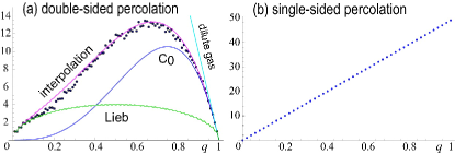
Figure 4: (Color online) The number of the zero energy states. The unit cell size is 100. The average is taken 1000 times.

We give physical interpretations of the zero modes. In the low density hydrogenation limit ($q\approx 0$), all sites are connected, i. e. the cluster number is only one. We can apply the Lieb theorem, which states that the number of the zero energy states is determined by the difference of the A-site and B-site. It is exactly obtained as

$$N_{0}^{\text{L}}=\sum_{s=0}^{M}\left|M-2s\right|\left(\begin{array}[]{c}N_{\text{c}}/2\\ s\end{array}\right)\left(\begin{array}[]{c}N_{\text{c}}/2\\ M-s\end{array}\right)\left(\begin{array}[]{c}N_{\text{c}}\\ M\end{array}\right)^{-1}$$ (2)

in terms of binomial coefficients. The distribution is symmetric at $M=N_{\text{c}}/2$. We have shown $N_{0}^{\text{L}}$ by the choice of $N_{\text{c}}=100$ in Fig.4(a). By taking $N_{\text{c}}\rightarrow\infty$, we obtain

$$N_{0}^{\text{L}}=\sqrt{2N_{\text{c}}pq/\pi}.$$ (3)

On the other hand, in the high density hydrogenation limit ($q\approx 1$), we can apply the dilute gas model. Every sites are isolated or unconnected with each other and give zero energy states. Then the number of zero is simply given by

$$N_{0}^{\text{D}}=N_{\text{c}}(1-q).$$ (4)

We have shown $N_{0}^{\text{D}}$ by the choice of $N_{\text{c}}=100$ in Fig.4(a).

A simple interpolating formula reads as

$$N_{0}\simeq C_{0}+\frac{1}{6}C_{1}+\frac{C_{2}+C_{3}}{C_{0}+C_{1}+C_{2}+C_{3}}N_{0}^{L},$$ (5)

where $C_{0}$, $C_{1}$, $C_{2}$ and $C_{3}$ are the numbers of isolated carbons, edge carbons, corner carbons and bulk carbons, respectively. It explains the numerical result reasonably well, as in Fig.4(a). The first and second terms represent the contributions from the isolated and edge carbons, respectively. The third term follows from the Lieb theorem with an appropriate correction.

We now discuss the zero-energy states in single-sided percolation. The number of the zero-energy states in each cluster is given by $N_{0}^{\text{cluster}}=\left|N_{B}^{\text{cluster}}-N_{A}^{\text{cluster}}\right|$ in general. Here, $N_{B}^{\text{cluster}}>N_{A}^{\text{cluster}}$ since only A sites are hydrogenated. Hence, the total number of the zero-energy states is given by

$$N_{0}=\sum N_{0}^{\text{cluster}}=N_{B}-N_{A}=qN_{\text{c}}.$$ (6)

This is confirmed perfectly by the numerical result in Fig.4(b). Thus, the numbers of the zero-energy states are very different between one-sided and double-sided hydrogenations.

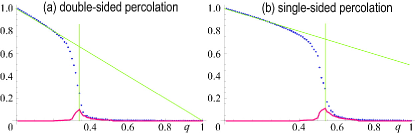
Figure 5: (Color online) The maximum cluster size (black dots) and the second maximum cluster size (red curves) for various hydrogenation density $q$ in unit of $N_{c}$. The unit cell size is 10000. The average is taken 100 times.

Metal-insulator transition: The bulk electronic properties of hydrographene is closely related to the connectivity of graph. We have calculated numerically the maximum cluster size $N^{\text{mc}}$ as a function of hydrogenation in the system with $N_{\text{c}}=10^{4}$, which we show in Fig.5. The ratio $N^{\text{mc}}/N_{\text{c}}$ is approximately equals to the percolation probability $P(q)$. It is by definition the probability for an infinitely large cluster to appear in an infinitely large system. In the present system it may be interpreted as a probability that the right-hand side and the left-hand side of a hydrographene sheet is connected by a cluster.

It is seen in Fig.5 that the maximum cluster size decreases almost linearly as $q$ increases, and suddenly becomes zero at a critical density $q_{c}$. This is a characteristic feature of a phase transition. Indeed, it is a phase transition since the present percolation system is mapped to the ferromagnet as we point out later: See (9). For double-sided percolation the critical density is determined as $q_{c}=0.32$, which is consistent with the well-known resultPercoBook on percolation in the honeycomb lattice. For single-sided percolation the critical density is determined as $q_{c}=0.55$.

The percolation probability is closely related to the conductance of hydrographene. For $q<q_{c}$, there is a large cluster around the sample. Thus the hydrographene is metallic. On the other hand, the hydrographene is insulator for $q>q_{c}$ because there is no such cluster. Namely, a percolation-induced metal-insulator transition occurs at $q=q_{c}$. It is intriguing that there is a large amount of the zero-energy states even though $q>q_{c}$. This is highly contrasted with the normal metal, where the metal or insulator can be determined by the existence of the zero-energy states. In hydrographene, the connectivity of carbon network plays a crucial role for the metal-insulator transition.

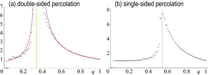
Figure 6: (Color online) The mean finite cluster size for various hydrogenation density $q$. The unit cell size is 40000. The average is taken 100 times.

We have also calculated numerically the mean size of finite cluster $S\left(q\right)$ as a function of hydrogenation, which we show in Fig.6. It diverge at $q_{c}=0.31$, indicating a critical behavior

$$S\left(p\right)\varpropto\left|q-q_{c}\right|^{-1}$$ (7)

for double-sided hydrogenation.

Magnetization: We proceed to analyze the magnetic property of hydrographene. We are able to make a general argument with respect to the magnetic moment. According to the Lieb theorem valid to the bipartite system at half-filling in connected graph, the magnetization $M$ is determined by the difference between the numbers $N_{A}$ and $N_{B}$ of the A and B sites in each cluster, $M=\frac{1}{2}\left|N_{A}-N_{B}\right|$, where the spin direction is arbitrary in general. The magnetization of hydrographene is determined by that of the largest cluster, since it is dominant: See Fig.5. We show the numerically calculated magnetization as a function of $q$ in Fig.7. It is well approximated by the relation

$$M(q)=P\left(q\right)N_{0}^{\text{L}},$$ (8)

where $N_{0}^{\text{L}}$ is given by eq.(3) for double-sided hydrogenation and eq.(6) for single-sided hydrogenation: See Fig.7(b). The system is ferromagnet for $q<q_{c}$, and paramagnet for $q>q_{c}$.

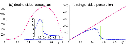
Figure 7: (Color online) The magnetization in unit of $\hbar/2$ in the presence (red dots) and absence (blue dots) of ferromagnetic coupling for various hydrogenation density $q$. A black curve represents the formula (8). Inset: An extended figure of the magnetization without ferromagnetic coupling. The unit cell size is 10000. The average is taken 500 times.

The maximum magnetization per site is obtained $M=3\times 10^{-3}$ at $q=0.21$ for double-sided hydrogenation and $M=0.17$ at $q=0.44$ for single-sided hydrogenation. Single-sided hydrogenation is about 500 times more efficient than double-sided hydrogenation because only A sites are hydrogenated in single-sided hydrogenation. The magnetization is proportional to the number of the sites. In other words, hydrographene shows the bulk magnetism, which is highly contrasted with the edge magnetism in graphene nanoribbons and nanodisks, where magnetization is proportional to the number of carbons along the edge. Bulk magnetism is desirable because edge magnetism disappears in the thermodynamic limit.

A comment is in order. It is intriguing that the magnetization is zero for the perfect single-sided hydrographene ($q=1$), which is in contradiction with the previous resultZhou obtained based on a density functional theory study. This is not surprising since the direction of magnetization is arbitrary in each cluster in our noninteracting model, as we have noted. The spin directions of two adjacent clusters may be aligned due to an exchange interaction if it is present, and it is probable that all clusters have the same spin direction. The maximum magnetization per site is obtained $M=0.13$ at $q=0.68$ for double-sided hydrogenation: See Fig.7(a). On the other hand, the magnetization increases linearly as a function of the hydrogenation parameter $q$ for single-sided hydrogenation: See Fig.7(b). This reproduces the resultZhou for the perfect single-sided hydrographene ($q=1$).

Percolation and ferromagnet: There exists a close relation between the percolation problem and the ferromagnet. Indeed, the percolation problem is mapped to the zero-state Potts model on Kagomé lattice via the Kasteleyn-Fortuin mappingKF . The hydrogenation parameter $q$ corresponds to the temperature $T$ of a ferromagnet,

$$q=\exp\left(-J/kT\right),$$ (9)

with $J$ being the exchange stiffness. The percolation probability $P\left(q\right)$ is mapped to the magnetization as a function of temperature $T$. Thus, the metal-insulator transition corresponds to the ferromagnet-paramagnet transition. Furthermore, the critical behavior (7) corresponds to the Curie-Weiss law of the susceptibility. We anticipate various properties familiar in ferromagnet to be translated into hydrographene via the Kasteleyn-Fortuin mapping.

In summary, we have discovered various intriguing electronic and magnetic properties of hydrographene based on a quantum-percolation model. We have proposed a new-type of percolation, single-sided percolation, which is qualitatively different from the usual percolation on honeycomb lattice. Hydrographene is an ideal system to investigate from the viewpoint of quantum site-percolation transition.

I am very much grateful to N. Nagaosa for fruitful discussions on the subject. This work was supported in part by Grants-in-Aid for Scientific Research from the Ministry of Education, Science, Sports and Culture No. 22740196.

References

- (1) K. S. Novoselov, et al., Science 306, 666 (2004). K. S. Novoselov, et al., Nature 438, 197 (2005). Y. Zhang, et al., Nature 438, 201 (2005).
- (2) A. H. Castro Neto, F. Guinea, N. M. R. Peres, K. S. Novoselov and A. K. Geim, Rev. Mod. Phys. 81, 109 (2009).
- (3) M. Fujita, et al., J. Phys. Soc. Jpn. 65, 1920 (1996), M. Ezawa, Phys. Rev. B, 73, 045432 (2006), L. Brey, and H. A. Fertig, Phys. Rev. B, 73, 235411 (2006).
- (4) M. Ezawa, Phys. Rev. B 76, 245415 (2007): M. Ezawa, Physica E 40, 1421-1423 (2008), J. Fernández-Rossier, and J. J. Palacios, Phys. Rev. Lett. 99, 177204 (2007), W. L. Wang, S. Meng and E. Kaxiras, Nano Letters 8, 241 (2008), P. Potasz, A. D. Güçlü and P. Hawrylak, Phys. Rev. B 81, 033403 (2010).
- (5) J.O. Sofo, A.S. Chaudhari, G.D. Barber, Phys. Rev. B 75, 153401 (2007).
- (6) D. C. Elias, R. R. Nair, T. M. G. Mohiuddin, S. V. Morozov, P. Blake, M. P. Halsall, A. C. Ferrari, D. W. Boukhvalov, M. I. Katsnelson, A. K. Geim, K. S. Novoselov, Science 323, 610 (2009).
- (7) R. Balog, B. Jorgensen, L. Nilsson, M. Andersen, E. Rienks, M. Bianchi, M. Fanetti, E. Lagsgaard, A. Baraldi, S. Lizzit, Z. Sljivancanin, F. Besenbacher, B. Hammer, T. G. Pedersen, P. Hofmann and L. Hornekar, Nature Materials 9, 315 (2010).
- (8) A Savchenko, Science 323, 589 (2009).
- (9) K. S. Novoselov, Physics World 27-30 Aug. (2009).
- (10) D. Stauffer, "Introduction to Percolation Theory" (Taylor & Francis, London, 1985).
- (11) J. Zhou, Q. Wang, Q. Sun, X. S. Chen, Y. Kawazoe and P. Jena, Nano Lett. 9, 3867 (2009).
- (12) P.W. Kasteleyn and C.M. Fortuin, J. Phys. Soc. Japan 26 (Suppl.) 11 (1969): C.M. Fortuin and P.W. Ksteleyn, Physica 57, 536 (1972).