Loschmidt echo in one-dimensional interacting Bose gases

Abstract

We explore Loschmidt echo in two regimes of one-dimensional (1D) interacting Bose gases: the strongly interacting Tonks-Girardeau (TG) regime, and the weakly-interacting mean-field regime. We find that the Loschmidt echo of a TG gas decays as a Gaussian when small perturbations are added to the Hamiltonian (the exponent is proportional to the number of particles and the magnitude of a small perturbation squared). In the mean-field regime the Loschmidt echo decays faster for larger interparticle interactions (nonlinearity), and it shows richer behavior than the TG Loschmidt echo dynamics, with oscillations superimposed on the overall decay.

I Introduction

The understanding of why an isolated (interacting many-body) system, which is initially say far from equilibrium, in many cases macroscopically undergoes irreversible evolution towards an equilibrium state, despite the fact that the microscopic laws are reversible, has intrigued scientists ever since the first disputes between Boltzmann and Loschmidt on this topic Loschmidt ; Boltzman . In principle, if the time was reversed at a given instance, the system would evolve back into the initial state. However, such a reversal is for all practical purposes impossible due to high sensitivity to small errors and interaction of the system with the environment. The quantity that measures sensitivity of quantum motion to perturbations is called Loschmidt echo or fidelity Peres ; Rodolfo ; Jacquod ; Cerruti ; Prosen (for a review see e.g. Gorin ). Fidelity tells us what is the probability that system will end up in the initial state after forward evolution for time $t$, followed by the slightly imperfect time reversed evolution for the same time $t$. In quantum mechanics time evolution from an initial state $\psi_{0}$ is given by the unitary operator $\hat{U}(t)=\exp(-i\hat{H}t/\hbar)$ via $\psi(t)=\exp(-i\hat{H}t/\hbar)\psi_{0}$, and the echo dynamics can be formally written as

$$F(t)=|\langle\psi_{0}|\exp(i\hat{H^{\prime}}t/\hbar)\exp(-i\hat{H}t/\hbar)|\psi_{0}\rangle|^{2}.$$ (1)

Here $\hat{H}$ is the Hamiltonian of the unperturbed system, and $\hat{H^{\prime}}=\hat{H}+\hat{V_{\varepsilon}}$ is the slightly perturbed Hamiltonian Gorin . One can think about this quantity as measuring the stability of quantum motion Peres , i.e., it tells us the overlap of the two states $\psi(t)$ and $\psi^{\prime}(t)$, the former is evolved forward in time by $\hat{H}$, and the latter by $\hat{H^{\prime}}$:

$$F(t)=|\langle\psi^{\prime}(t)|\psi(t)\rangle|^{2}.$$ (2)

In quantum systems, depending on the strength of the perturbation and the properties of the nonperturbed Hamiltonian, three different decay regimes of Loschmidt echo are usually identified: the Gaussian perturbative regime Jacquod ; Cerruti , the exponential Fermi golden rule regime Jacquod ; Cerruti ; Prosen ; Rodolfo , and the Lyapunov regime Rodolfo .

Motivated by the recent progress in experiments and theory on ultracold atomic gases Bloch2008 , where the influence of the environment can be made very small, and the strength of the atom-atom interactions can be tuned Bloch2008 , we are motivated to investigate Loschmidt echo dynamics in those systems. In particular, we focus on one-dimensional (1D) Bose gases which were experimentally realized OneD even in the strongly correlated regime of Tonks-Girardeau (TG) bosons TG2004 ; Kinoshita2006 , both in TG2004 and out of equilibrium Kinoshita2006 . The realization of the TG gas in atomic waveguides was proposed by Olshanii Olshanii . The 1D atomic gases can be described with the Lieb-Liniger model Lieb1963 , which for weak interactions is well-described by the Nonlinear Schrödinger equation (Gross-Pitaevskii theory) Bloch2008 , whereas for sufficiently strong interactions one enters the Tonks-Girardeau regime, where exact solutions can be found via Fermi-Bose mapping Girardeau1960 . This method was used to study out-of-equilibrium dynamics in the strongly correlated regime (e.g., see Girardeau2000 ; Rigol2005 ; Minguzzi2005 ; Rigol2006 ; delCampo2006 ; Pezer2007 ). The Loschmidt echo was within the mean-field Gross-Pitaevskii theory addressed in Refs. Manfredi2008 ; Martin2008 . We would also like to point out at a study of orthogonality catastrophe (and the relation to Loschmidt echo) in an ultracold Fermi gas coupled to a single cubit Goold2011 .

Here we demonstrate, with exact numerical calculation, that for small random stationary perturbation, the Loschmidt echo for a TG gas decays as a Gaussian with decay constant proportional to the number of particles and the square of the amplitude of the perturbation. We analytically derive the Gaussian behavior of TG fidelity within approximation presented by Peres Peres . In the mean-field regime the Loschmidt echo decays faster for larger interparticle interactions (nonlinearity), and it shows richer behavior than the TG Loschmidt echo dynamics, with oscillations superimposed on the overall decay.

II The physical system and the corresponding model

Consider a gas of $N$ identical bosons in a one-dimensional (1D) space, which interact via pointlike interactions, described by the Hamiltonian

$$H=\sum_{i=1}^{N}\left[-\frac{\hbar^{2}}{2m}\frac{\partial^{2}}{\partial X_{i}^{2}}+U(X_{i})\right]+g_{1D}\sum_{1\leq i<j\leq N}\delta(X_{i}-X_{j}).$$ (3)

Such a system can be realized with ultracold bosonic atoms trapped in effectively 1D atomic waveguides OneD ; TG2004 ; Kinoshita2006 , where $U(X)$ is the axial trapping potential, and $g_{1D}=2\hbar^{2}a_{3D}[ma_{\bot}^{2}(1-Ca_{3D}/\sqrt{2}a_{\bot})]^{-1}$ is the effective 1D coupling strength; $a_{3D}$ stands for the three-dimensional s-wave scattering length, $a_{\bot}=\sqrt{\hbar/m\omega_{\bot}}$ is the transverse width of the trap, and $C=1.4603$ Olshanii . By varying $\omega_{\bot}$ the system can be tuned from the mean field regime described by the Gross-Pitaevskii equation, up to the strongly-interacting Tonks-Girardeau regime ($g_{1D}\rightarrow\infty$). In equilibrium, different regimes of these 1D gases are usually characterized by a dimensionless parameter $\gamma=mg_{1D}/\hbar^{2}n_{1D}$, where $n_{1D}$ stands for the linear atomic density. For $\gamma\ll 1$ the gas is in mean field regime and for $\gamma\gg 1$ it is in the strongly interacting regime (we consider repulsive interactions $\gamma>0$) Lieb1963 ; Olshanii ; TG2004 ; Kinoshita2006 . One can tune $\gamma$ by say changing the transverse confinement frequency. In our calculations, we use Hamiltonian (3) in its dimensionless form

$$H=\sum_{i=1}^{N}\left[-\frac{\partial^{2}}{\partial x_{i}^{2}}+V(x_{i})\right]+2c\sum_{i<j}^{N}\delta(x_{i}-x_{j}).$$ (4)

where $x=X/X_{0}$ ($X_{0}$ is the spatial scale which we choose to be $1\,\mu$m). Here we consider ⁸⁷Rb atoms with the 3D scattering length $a_{3D}=5.3$ nm TG2004 ; Kinoshita2006 . Energy is in units of $E_{0}=\hbar^{2}/2mX_{0}^{2}=3.82\cdot 10^{-32}$ J, and time is in units of $T_{0}=2mX_{0}^{2}/\hbar=2.8$ ms. The dimensionless axial potential is $V(x)=U(X)/E_{0}$, and the interactions strength parameter is $2c=g_{1D}/X_{0}E_{0}$.

III Loschmidt echo of a Tonks-Girardeau gas

For the Tonks-Girardeau gas, the interaction strength is infinite $c\rightarrow\infty$, that is, the bosons are ”impenetrable” Girardeau1960 . Consequently, an exact (static and time-dependent) solution of this model can be written via Girardeau’s Fermi-Bose mapping Girardeau1960 ; Girardeau2000

$$\psi_{B}(x_{1},\ldots,x_{N},t)=\prod_{1\leq i<j\leq N}\mbox{sgn}(x_{i}-x_{j})\psi_{F}(x_{1},\ldots,x_{N},t),$$ (5)

where $\psi_{F}$ denotes a wave function describing $N$ noninteracting spin polarized fermions in the external potential $V(x)$. In our simulations we consider up to $N=70$ particles. The system is initially (for times $t\leq 0$) in the ground state of a container like potential,

$$V_{L}(x)=V_{0}\{1+\tanh[V_{s}(x-L/2)]/2-\tanh[V_{s}(x+L/2)]/2\},$$ (6)

where $V_{0}=500$, $V_{s}=4$, and $L=15$ (corresponding to $15\,\mu$m). At $t=0$ we suddenly expand the width of the container to twice its original width, that is, the potential at times $t>0$ is $V_{2L}(x)$. In order to calculate the fidelity $F(t)$, we must evolve the TG gas in the new potential $V_{2L}(x)$, and in the potential $V_{2L}^{\prime}(x)=V_{2L}(x)+V_{\varepsilon}(x)$ starting from identical initial states. Here $V_{\varepsilon}(x)$ is a small noise potential of amplitude $\varepsilon$. The Loschmidt echo $F(t)=|\langle\psi_{B}^{\prime}(t)|\psi_{B}(t)\rangle|^{2}$ is calculated from the knowledge of the TG many-body states $\psi_{B}(t)$ and $\psi_{B}^{\prime}(t)$ corresponding to the evolution in potentials $V_{2L}(x)$ and $V_{2L}^{\prime}(x)$, respectively.

The fermionic wave function $\psi_{F}$ can in our case be written as a Slater determinant, $\psi_{F}(x_{1},\ldots,x_{N},t)=\det_{m,n=1}^{N}[\psi_{m}(x_{n},t)]/\sqrt{N!}$, where $\psi_{m}(x,t)$, $m=1,\ldots,N$, satisfy the single-particle Schrödinger equation

$$i\frac{\partial\psi_{m}(x,t)}{\partial t}=\left[-\frac{\partial^{2}}{\partial x^{2}}+V_{2L}(x)\right]\psi_{m}(x,t),$$ (7)

and equivalently for $\psi_{m}^{{}^{\prime}}(x,t)$ which evolve in $V_{2L}^{\prime}(x)$. The initial conditions are such that $\psi_{m}(x,0)=\psi_{m}^{{}^{\prime}}(x,0)$ is the $m$-th single particle eigenstate of the initial container potential $V_{L}(x)$. The Loschmidt echo for a Tonks-Girardeau gas can be written in a form convenient for calculation:

$$|\langle\psi_{B}^{\prime}(t)|\psi_{B}(t)\rangle|^{2} = |\frac{1}{N!}\int dx_{1}\cdots dx_{N}\sum_{\sigma_{1}}(-)^{\sigma_{1}}\prod_{i=1}^{N}\psi^{{}^{\prime}*}_{\sigma_{1}(i)}(x_{i},t)\sum_{\sigma_{2}}(-)^{\sigma_{2}}\prod_{j=1}^{N}\psi_{\sigma_{2}(j)}(x_{j},t)|^{2}$$ (8)

$$= |\frac{1}{N!}\sum_{\sigma_{1}}\sum_{\sigma_{2}}(-)^{\sigma_{1}}(-)^{\sigma_{2}}\prod_{i=1}^{N}P_{\sigma_{1}(i)\sigma_{2}(i)}(t)|^{2}$$

$$= |\det\mathbf{P}(t)|^{2},$$

where $\sigma$ denotes a permutation in $N$ indices, $(-)^{\sigma}$ is its signature, and

$$P_{ij}(t)=\int\psi_{i}^{{}^{\prime}*}(x,t)\psi_{j}(x,t)dx.$$ (9)

In writing relation (8) we used a definition of the determinant. Since at $t=0$ we have $P_{ij}(0)=\delta_{ij}$, that motivates us to define the fidelity product

$$F_{P}(t)=\prod_{i=1}^{N}P_{ii}(t)P_{ii}^{*}(t).$$ (10)

Thus, in calculation of the fidelity product we assume that all off diagonal elements of the matrix (9) are zero i.e $P_{ij}(t)=0$ for $i\neq j$ for all times. It can be interpreted as if we evolve the $N$ particles fully independently of each other (including statistics) starting from the $N$ initial states $\psi_{m}(x,0)$, $m=1,\ldots,N$, calculate $N$ different fidelities for these states, and multiply them to obtain the product fidelity. The value $F(t)$ is identical for noninteracting spinless fermions and interacting TG bosons; note that Eq. (8) is identical to the formula used by Goold et al. in Ref. Goold2011 studying the orthogonality catastrophe for ultracold fermions. Thus, $F_{P}$ and $F$ will distinguish the influence of antysymmetrization in the case of noninteracting fermions, or TG interactions and symmetrization in the case of bosons, with dynamics which does not include neither statistics nor interactions into account. We would like to emphasize that derivation of (8) and (9) does not require that we initiate the dynamics from the ground state of the TG gas in the initial trap; we could have chosen any excited TG eigenstate as initial condition as well.

In order to calculate the fidelity $F(t)$, we must evolve the single particle states $\psi_{j}(x,t)$ [$\psi_{j}^{{}^{\prime}}(x,t)$, respectively], in the potential $V_{2L}(x)$ [$V_{2L}(x)+V_{\varepsilon}(x)$], starting from the first $N$ single-particle eigenstates of $V_{L}(x)$. The evolution is performed via standard linear superposition in terms of the eigenstates $\phi_{m}(x)$ of the final container potential $V_{2L}(x)$ (which are calculated numerically):

$$\psi_{j}(x,t)=\sum_{m}a_{m}^{j}\phi_{m}(x)\exp(-iE_{m}t),$$ (11)

and

$$\psi_{j}^{\prime}(x,t)=\sum_{m}a_{m}^{j^{\prime}}\phi_{m}^{\prime}(x)\exp(-iE_{m}^{\prime}t).$$ (12)

We numerically calculate the coefficients $a_{n}^{j^{\prime}}=\int\phi_{m}^{{}^{\prime}*}(x)\psi_{j}(x,0)dx$ and $a_{n}^{j}=\int\phi_{m}^{*}(x)\psi_{j}(x,0)dx$ for $j=1,\ldots,70$, and $m=1,\ldots,210$ which is sufficient for the parameters we used. The noise potential is constructed as follows: $x$-space is numerically simulated by using $2048$ equidistant points in the interval $x\in[-30,30]$. From this array we construct a random array $V_{\textrm{rand}}(x)=|FT^{-1}[\exp(-k^{4}/K_{cut}^{4})FT[\textrm{rand}(x)]]|$ of the same length, where $\textrm{rand}(x)$ is a random number between $0$ and $1$, $FT$ stands for the Fourier transform, $K_{cut}$ is the cut-off wave vector (set to $K_{cut}=53$) introduced to make the discrete numerical potential sufficiently ”smooth” from point to point. Finally the noise potential is obtained via $V_{\varepsilon}(x)=\varepsilon[V_{\textrm{rand}}(x)-\bar{V}_{\textrm{rand}}]$, where $\varepsilon$ is the amplitude of the perturbation, and $\bar{V}_{\textrm{rand}}$ is the mean value of $V_{\textrm{rand}}(x)$. Such a potential can be constructed optically for 1D Bose gases Billy2008 .

The fidelity depends on the particle number $N$, the amplitude of noise $\varepsilon$, but also on the particular realization of $V_{\varepsilon}(x)$, hence, we calculate all quantities (e.g., the Loschmidt echo) for 50 different realizations of $V_{\varepsilon}(x)$, and then perform the average over the noise ensemble: $\langle F(t)\rangle_{noise}$.

In Fig. 1(a) we show the fidelity $\langle F(t)\rangle_{noise}$ as a function of time, for three different numbers of particles, $N=10$, $20$ and $50$ with $\varepsilon=0.05$. We find that in the TG regime, the Loschmidt echo decays as a Gaussian: $\langle F(t)\rangle_{noise}=\exp(-\langle\lambda(N,\varepsilon)\rangle t^{2})$; solid black lines represent the Gaussian curves fitted to the numerically obtained values. We point out that in every single realization of the noise, the fidelity for a TG gas decays as a Gaussian, with small fluctuations in the value of the exponent. The error bars in Fig. 1(a) represent the standard deviation of the fidelity at a given time. Note that the standard deviation gets smaller with increasing particle number $N$, which means that for sufficiently large $N$ it suffices to calculate fidelity decay for a single realization of the potential to obtain reliable values for $\lambda(N,\varepsilon)$. It s interesting to compare the fidelity with the fidelity-product $\langle F_{P}(t)\rangle_{noise}$, which can also be fitted well with the Gaussian function as illustrated in Fig. 1(b). We find that the product $\langle F_{P}(t)\rangle_{noise}$ is systematically below the value of the fidelity.

In Fig. 2 we depict the dependence of the fidelity, that is, of the exponent $\langle\lambda(N,\varepsilon)\rangle$, on the number of particles $N$ and $\varepsilon$. In Fig. 2(a) we plot $\langle\lambda(N,\varepsilon)\rangle/\varepsilon^{2}$ as a function of $\varepsilon$ for different values of $N$; evidently we have $\langle\lambda(N,\varepsilon)\rangle\propto\varepsilon^{2}$. In Fig. 2(b) we plot $\langle\lambda(N,\varepsilon)\rangle/N$ as a function of $N$ for $\varepsilon=0.05$; we clearly see that $\langle\lambda(N,\varepsilon)\rangle\propto N$ for sufficiently large $N$ (already for $N>20$).

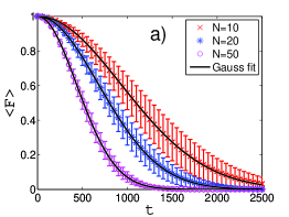
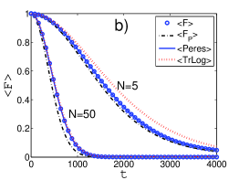
Figure 1: (color online) Decay of the Loschmidt echo (fidelity) with time for $\varepsilon=0.05$. (a) The averaged values $\langle F(t)\rangle_{noise}$ for $N=10$ (crosses), $N=20$ (asterisks), and $N=50$ (circles). Solid black lines represent the Gaussian functions fitted to the numerically obtained values. Error bars depict the standard deviation for 50 different realizations of the noise potential $V_{\varepsilon}(x)$. (b) The fidelity $\langle F(t)\rangle_{noise}$ (circles), fidelity product $\langle F_{P}(t)\rangle_{noise}$ (black dot-dashed lines), the values obtained via $\det(\mathbf{PP}^{\dagger})$, where $P_{ij}=\sum_{n}a_{n}^{i*}a_{n}^{j}\exp(i\omega_{n}t)$ is obtained via approximation presented by Peres Peres (blue line), and the fidelity obtained via trace-log formula Eq. (14) (red dotted line).

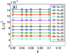
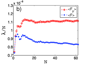
Figure 2: (color online) The Gaussian exponent of the fidelity as a function of $\varepsilon$ and $N$. (a) The quantities $\langle\lambda\rangle/\varepsilon^{2}$ are plotted for different particle numbers, and they are ordered just as in the legend (higher lines are for larger values of $N$); obviously $\langle\lambda\rangle\propto\varepsilon^{2}$. (b) The quantities $\langle\lambda_{P}\rangle/N$ (red circles, upper line) and $\langle\lambda\rangle/N$ (blue asterisks, lower line), are plotted as a function of $N$ for $\varepsilon=0.05$. For larger $N$ the lines become horizontal indicating that $\langle\lambda\rangle\propto N\propto\langle\lambda_{P}\rangle$.

In order to understand numerical results of Fig. 1 and Fig. 2, we analytically explore the properties of the fidelity for a single realization of $V_{\varepsilon}(x)$. To this end we use an approximation from Peres Peres , where to first order in $\varepsilon$ one has $\int dx\phi_{j}^{{}^{\prime}*}\phi_{i}\approx\delta_{ij}$, and $a_{m}^{j}\approx a_{m}^{j^{\prime}}$. The elements of the matrix $\mathbf{P}$, which yield the fidelity via Eq. (8), are then written as $P_{ij}=\sum_{n}a_{n}^{i*}a_{n}^{j}\exp(i\omega_{n}t)$, where $\omega_{n}=E_{n}^{\prime}-E_{n}\approx\langle\phi_{n}|V_{\varepsilon}|\phi_{n}\rangle$. In Fig. 1(b) we plot the fidelity obtained with this approximation (blue line) and the one obtained with the exact numerical evolution (blue circles); the agreement is excellent. The diagonal elements $|P_{ii}(t)|^{2}$ can be interpreted as single-particle fidelities corresponding to the initial states $\psi_{i}(x,0)$. It is straightforward to see that $|P_{ii}(t)|^{2}=\sum_{n,m}|a_{n}^{i}|^{2}|a_{m}^{i}|^{2}\cos[(\omega_{n}-\omega_{m})t]$, however, we note that in our simulations only a few terms contribute to the sum above, yielding oscillatory behavior of the single particle fidelities with relatively high amplitudes of the oscillation. Now we turn to the TG gas and our observation that the decay of fidelity is Gaussian. In order to derive this we use the trace-log formula for the determinants:

$$F(t)=\exp(\textrm{Tr}(\log(\mathbf{PP}^{\dagger}))).$$ (13)

We can approximate $\mathbf{PP}^{\dagger}\approx\mathbf{1}+\mathbf{Q_{1}}t-\mathbf{Q_{2}}t^{2}+\mathcal{O}(t^{3})$, where $\Delta_{nm}=\omega_{n}-\omega_{m}$, $[Q_{1}]_{ij}=i\sum_{k=1}^{N}\sum_{n,m}a_{n}^{i*}a_{n}^{k}a_{m}^{j}a_{m}^{k*}\Delta_{nm}$, and $[Q_{2}]_{ij}=\frac{1}{2}\sum_{k=1}^{N}\sum_{n,m}a_{n}^{i*}a_{n}^{k}a_{m}^{j}a_{m}^{k*}\Delta_{nm}^{2}$. Next we expand the logarithm in trace-log formula which yields

$$F(t)=\exp(-\textrm{Tr}\mathbf{Q_{2}}t^{2}),$$ (14)

i.e., a Gaussian function. In our derivation we used $\textrm{Tr}\mathbf{Q_{1}}=0$. Red dotted line in Fig. 1(b) shows that Eq. (14) is an excellent approximation for larger $N$. The dependence of $\langle\lambda(N,\varepsilon)\rangle$ on $\varepsilon$ follows from the fact that $\Delta_{nm}^{2}\propto\varepsilon^{2}$, whereas $\textrm{Tr}\mathbf{Q_{2}}\propto N$ (see Fig. 2).

In the rest of this section we argue that $F_{P}(t)<F(t)$, i.e., that the fidelity product is smaller than the fidelity. Obviously we need only diagonal elements of matrix $\mathbf{PP}^{\dagger}$ to construct either $F(t)$ or $F_{P}(t)$, which we write as

$$(\mathbf{PP}^{\dagger})_{ii}=|P_{ii}(t)|^{2}+\sum_{k=1,k\neq i}^{N}|P_{ik}(t)|^{2}.$$ (15)

For the first term we can write $|P_{ii}(t)|^{2}=1-\alpha_{i}(t)$ where $\alpha_{i}(t)$ is some function of time with properties $\alpha_{i}(0)=0$ and $0\leq\alpha_{i}(t)\leq 1$ due to relation (9). For the second term we write $\sum_{k=1,k\neq i}^{N}|P_{ik}(t)|^{2}=\beta_{i}(t)$ where $\beta_{i}(0)=0$ and $\beta_{i}(t)\geq 0$. It follows that $(\mathbf{PP}^{\dagger})_{ii}=1-(\alpha_{i}(t)-\beta_{i}(t))$. By applying the trace-log formula in the same manner as before, we get for the fidelity $F(t)=\exp(-\sum_{i=1}^{N}\alpha_{i}(t)+\sum_{i=1}^{N}\beta_{i}(t))$. The fidelity product corresponds to $\exp(-\sum_{i=1}^{N}\alpha_{i}(t))$, which yields $F(t)=F_{P}(t)\exp(\sum_{i=1}^{N}\beta_{i}(t))$; since $\sum_{i=1}^{N}\beta_{i}(t)\geq 0$ we have $F(t)\geq F_{P}(t)$. Averaging over noise does not change this relation.

IV Fidelity in the mean field regime

In this section we consider Loschmidt echo in the mean field regime, that is, by employing the Gross-Pitaevskii theory. The dynamics of Bose-Einsten condensates (BECs) is within the framework of this theory described by using the nonlinear Schrödinger equation (NLSE), which we write in dimensionless form:

$$i\frac{\partial\Phi(x,t)}{\partial t}=\left[-\frac{\partial^{2}}{\partial x^{2}}+V(x)\right]\Phi(x,t)+\tilde{g}_{1D}N|\Phi(x,t)|^{2}\Phi(x,t),$$ (16)

where $\tilde{g}_{1D}=2mX_{0}g_{1D}/\hbar^{2}$ is the dimensionless coupling strength and $\int|\Phi(x,t)|^{2}dx=1$; here we choose $\tilde{g}_{1D}=0.04$, which can be experimentally obtained by tuning the transverse confinement frequency to $\omega_{\bot}/2\pi\approx 240$ Hz, and with $N=50$. With those parameters the system is in the mean field regime with $\gamma\approx 0.01$. All parameters are identical as in the simulations of a TG gas, except that now $\omega_{\bot}$ is smaller.

To compute the fidelity of interacting BECs we repeat the same procedure as for the TG gas: first we prepare the condensate in the ground state of the container like potential $V_{L}(x)$ (i.e. we solve numerically the stationary NLSE), second we suddenly expand the container to $V_{2L}(x)$, and solve numerically the time-dependent NLSE in the expanded potential without noise [$V_{2L}(x)$], and with noise [$V_{2L}^{\prime}(x)$], with identical initial conditions. This gives us $\Phi(x,t)$ and $\Phi^{\prime}(x,t)$ from which we calculate the fidelity

$$F_{GP}(t)=|\int\Phi^{{}^{\prime}*}(x,t)\Phi(x,t)dx|^{2}.$$ (17)

However, note that since we investigate the fidelity of a gas with $N$ particles, the mean-field $N$-particle wavefunction is a product state, $\psi_{GP}(x_{1},\ldots,x_{N},t)=\prod_{j=1}^{N}\Phi(x_{j},t)$, and therefore the $N$-particle mean-field fidelity is

$$F_{GP}^{N}(t)=|\int\psi_{GP}^{{}^{\prime}*}\psi_{GP}dx_{1}\ldots dx_{N}|^{2}=[F_{GP}(t)]^{N}.$$ (18)

Finally, we average over 50 different realizations of the potential to obtain $\langle F_{GP}(t)\rangle_{noise}$ and $\langle F_{GP}^{N}(t)\rangle_{noise}$.

In Fig. 3(a) we plot $\langle F_{GP}(t)\rangle_{noise}$ and its standard deviation for noninteracting and weakly-interacting BECs. We see that oscillations are superimposed on the overall decay in contrast to the TG gas case. We find that in the mean-field regime described by the Gross-Pitaevskii equation the fidelity decays faster for larger nonlinearity (interaction strength). It is worthy to point out that $F_{GP}(t)$ is very dependent on the particular realization of $V_{\varepsilon}(x)$, which is not the case for the TG gas. This is illustrated in Fig. 3(b) where we show dynamics of $F_{GP}(t)$ for two different realizations of the noise potential; we observe a large dependence of $F_{GP}(t)$ on a particular realization of the noise. This is a consequence of the fact that the oscillation frequency of fidelity $|P_{11}(t)|^{2}=\sum_{n,m}|a_{n}^{1}|^{2}|a_{m}^{1}|^{2}\cos[(\omega_{n}-\omega_{m})t]$ for the noninteracting BEC essentially depends on the difference between only several frequencies which is very noise sensitive, and this behavior is inherited in the nonlinear mean-field regime.

Finally, in Fig. 4 we compare the fidelities of the noninteracting BEC, the weakly-interacting BEC, and the TG gas. Note that for proper comparison one should compare $F_{GP}^{N}(t)$ with $F(t)$. We see that the mean-field fidelity shows richer behavior. In the regime of parameters we used, we find that $\langle F_{GP}^{N}(t)\rangle_{noise}$ decays faster than the TG regime fidelity in the first part of the decay dynamics, but later the mean-field regime fidelity decay slows down in comparison to the TG gas decay.

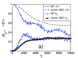
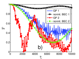
Figure 3: (a) Noise-averaged fidelities of evolving BECs for $N=50$ and $\varepsilon=0.05$, and standard deviations from the noise-average. The averaged fidelity for a noninteracting BEC is shown with the black dot-dashed line, and its standard deviation with open black circles. The averaged fidelity for a weakly-interacting BEC is shown with the blue solid line, and its standard deviation with closed blue circles. (b) Fidelities of the evolving BECs for two different realizations of the noise potential.

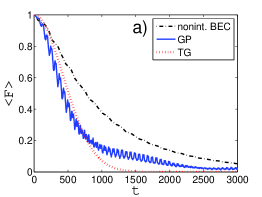
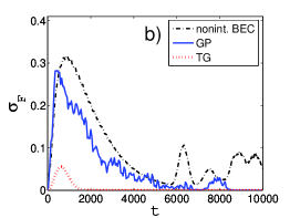
Figure 4: Comparison of the averaged fidelities (a) and their standard deviations (b) for the TG gas ($\langle F(t)\rangle_{noise}$, red dotted line), the weakly-interacting BEC ($\langle F_{GP}^{N}(t)\rangle_{noise}$, solid blue line), and the noninteracting BEC (black dot-dashed line), for the same number of particles. The parameters are $N=50$ and $\varepsilon=0.05$.

V Conclusion

In conclusion, we have explored Loschmidt echo (fidelity) in two regimes of one-dimensional interacting Bose gases: the strongly interacting TG regime, and the weakly-interacting mean-field regime described within the Gross-Pitaevskii theory. The gas is initially in the ground state of a trapping potential that is suddenly broadened, and the decay of fidelity is studied numerically by using a small spatial noise perturbation. We find (numerically and analytically) that the fidelity of the TG gas decays as a Gaussian with the exponent proportional to the number of particles and the magnitude of the small perturbation squared (see Fig. 1 and Fig. 2). Our results do not depend on the details of trapping potential; we have obtained the same behavior for a gas that is initially loaded in the ground state of the harmonic oscillator potential, which is subsequently suddenly broadened. Furthermore we find that Gaussian decay remains if we initiate the dynamics from some excited initial state or from a superposition of such states. In the mean-field regime the Loschmidt echo decays faster for larger interparticle interactions (nonlinearity), and it shows richer behavior than TG Loschmidt echo dynamics with oscillations superimposed on the overall decay (see Fig. 3 and Fig. 4); it also has much larger sensitivity on the noise (see Fig. 3(b)). Finally, we would like to mention that perhaps the most interesting regime of Loschmidt echo dynamics would be for intermediate Lieb-Liniger interactions, which seem to be exactly solvable only for specific external potential configurations Jukic .