Coordinate descent algorithms for nonconvex penalized regression, with applications to biological feature selection

Abstract

A number of variable selection methods have been proposed involving nonconvex penalty functions. These methods, which include the smoothly clipped absolute deviation (SCAD) penalty and the minimax concave penalty (MCP), have been demonstrated to have attractive theoretical properties, but model fitting is not a straightforward task, and the resulting solutions may be unstable. Here, we demonstrate the potential of coordinate descent algorithms for fitting these models, establishing theoretical convergence properties and demonstrating that they are significantly faster than competing approaches. In addition, we demonstrate the utility of convexity diagnostics to determine regions of the parameter space in which the objective function is locally convex, even though the penalty is not. Our simulation study and data examples indicate that nonconvex penalties like MCP and SCAD are worthwhile alternatives to the lasso in many applications. In particular, our numerical results suggest that MCP is the preferred approach among the three methods.

and

t1Supported in part by NIH Grant T32GM077973-05. t2Supported in part by NIH Grant R01CA120988 and NSF Grant DMS-08-05670.

1 Introduction

Variable selection is an important issue in regression. Typically, measurements are obtained for a large number of potential predictors in order to avoid missing an important link between a predictive factor and the outcome. This practice has only increased in recent years, as the low cost and easy implementation of automated methods for data collection and storage has led to an abundance of problems for which the number of variables is large in comparison to the sample size.

To reduce variability and obtain a more interpretable model, we often seek a smaller subset of important variables. However, searching through subsets of potential predictors for an adequate smaller model can be unstable [Breiman (1996)] and is computationally unfeasible even in modest dimensions.

To avoid these drawbacks, a number of penalized regression methods have been proposed in recent years that perform subset selection in a continuous fashion. Penalized regression procedures accomplish this by shrinking coefficients toward zero in addition to setting some coefficients exactly equal to zero (thereby selecting the remaining variables). The most popular penalized regression method is the lasso [Tibshirani (1996)]. Although the lasso has many attractive properties, the shrinkage introduced by the lasso results in significant bias toward 0 for large regression coefficients.

Other authors have proposed alternative penalties, designed to diminish this bias. Two such proposals are the smoothly clipped absolute deviation (SCAD) penalty [Fan and Li (2001)] and the mimimax concave penalty [MCP; Zhang (2010)]. In proposing SCAD and MCP, their authors established that SCAD and MCP regression models have the so-called oracle property, meaning that, in the asymptotic sense, they perform as well as if the analyst had known in advance which coefficients were zero and which were nonzero.

However, the penalty functions for SCAD and MCP are nonconvex, which introduces numerical challenges in fitting these models. For the lasso, which does possess a convex penalty, least angle regression [LARS; Efron et al. (2004)] is a remarkably efficient method for computing an entire path of lasso solutions in the same order of time as a least squares fit. For nonconvex penalties, Zou and Li (2008) have proposed making a local linear approximation (LLA) to the penalty, thereby yielding an objective function that can be optimized using the LARS algorithm.

More recently, coordinate descent algorithms for fitting lasso-penalized models have been shown to be competitive with the LARS algorithm, particularly in high dimensions [Friedman et al. (2007); Wu and Lange (2008); Friedman, Hastie and Tibshirani (2010)]. In this paper we investigate the application of coordinate descent algorithms to SCAD and MCP regression models, for which the penalty is nonconvex. We provide implementations of these algorithms through the publicly available R package, ncvreg (available at http://cran.r-project.org).

Methods for high-dimensional regression and variable selection have applications in many scientific fields, particularly those in high-throughput biomedical studies. In this article we apply the methods to two such studies—a genetic association study and a gene expression study—each possessing a different motivation for sparse regression models. In genetic association studies, very few genetic markers are expected to be associated with the phenotype of interest. Thus, the underlying data-generating process is likely to be highly sparse, and sparse regression methods likely to perform well. Gene expression studies may also have sparse underlying representations; however, even when they are relatively “dense,” there may be separate motivations for sparse regression models. For example, data from microarray experiments may be used to discover biomarkers and design diagnostic assays. To be practical in clinical settings, such assays must use only a small number of probes [Yu et al. (2007)].

In Section 2 we describe algorithms for fitting linear regression models penalized by MCP and SCAD, and discuss their convergence. In Section 3 we discuss the modification of those algorithms for fitting logistic regression models. Issues of stability, local convexity and diagnostic measures for investigating these concerns are discussed, along with the selection of tuning parameters, in Section 4. The numerical efficiency of the proposed algorithm is investigated in Section 5 and compared with LLA algorithms. The statistical properties of lasso, SCAD and MCP are also investigated and compared using simulated data (Section 5) and applied to biomedical data (Section 6).

2 Linear regression with nonconvex penalties

Suppose we have $n$ observations, each of which contains measurements of an outcome $y_{i}$ and $p$ features $\{x_{i1},\ldots,x_{ip}\}$. We assume without loss of generality that the features have been standardized such that $\sum_{i=1}^{n}x_{ij}=0$, $n^{-1}\sum_{i=1}^{n}x_{ij}^{2}=1$ and $\sum_{i=1}^{n}y_{i}=0$. This ensures that the penalty is applied equally to all covariates in an equivariant manner, and eliminates the need for an intercept. This is standard practice in regularized estimation; estimates are then transformed back to their original scale after the penalized models have been fit, at which point an intercept is introduced.

We will consider models in which the expected value of the outcome depends on the covariates through the linear function $\mathrm{E}(\mathbf{y})=\bolds{\eta}=\mathbf{X}\bolds{\beta}$. The problem of interest involves estimating the vector of regression coefficients $\bolds{\beta}$. Penalized regression methods accomplish this by minimizing an objective function $Q$ that is composed of a loss function plus a penalty function. In this section we take the loss function to be squared error loss:

$$Q_{\lambda,\gamma}(\bolds{\beta})=\frac{1}{2n}\sum_{i=1}^{n}(y_{i}-\eta_{i})^{2}+\sum_{j=1}^{p}p_{\lambda,\gamma}(|\beta_{j}|),$$ (1)

where $p_{\lambda,\gamma}(\cdot)$ is a function of the coefficients indexed by a parameter $\lambda$ that controls the tradeoff between the loss function and penalty, and that also may be shaped by one or more tuning parameters $\gamma$. This approach produces a spectrum of solutions depending on the value of $\lambda$; such methods are often referred to as regularization methods, with $\lambda$ the regularization parameter.

To find the value of $\bolds{\beta}$ that optimizes (1), the LLA algorithm makes a linear approximation to the penalty, then uses the LARS algorithm to compute the solution. This process is repeated iteratively until convergence for each value of $\lambda$ over a grid. Details of the algorithm and its implementation may be found in Zou and Li (2008).

The LLA algorithm is inherently inefficient to some extent, in that it uses the path-tracing LARS algorithm to produce updates to the regression coefficients. For example, over a grid of 100 values for $\lambda$ that averages 10 iterations until convergence at each point, the LLA algorithm must calculate 1000 lasso paths to produce a single approximation to the MCP or SCAD path.

An alternative to LLA is to use a coordinate descent approach. Coordinate descent algorithms optimize a target function with respect to a single parameter at a time, iteratively cycling through all parameters until convergence is reached. The idea is simple but efficient—each pass over the parameters requires only $O(np)$ operations. If the number of iterations is smaller than $p$, the solution is reached with even less computation burden than the $np^{2}$ operations required to solve a linear regression problem by QR decomposition. Furthermore, since the computational burden increases only linearly with $p$, coordinate descent algorithms can be applied to very high-dimensional problems.

Coordinate descent algorithms are ideal for problems that have a simple closed form solution in a single dimension but lack one in higher dimensions. The basic structure of a coordinate descent algorithm is, simply: For $j$ in $\{1,\ldots,p\}$, to partially optimize $Q$ with respect to $\beta_{j}$ with the remaining elements of $\bolds{\beta}$ fixed at their most recently updated values. Like the LLA algorithm, coordinate descent algorithms iterate until convergence is reached, and this process is repeated over a grid of values for $\lambda$ to produce a path of solutions.

The efficiency of coordinate descent algorithms comes from two sources: (1) updates can be computed very rapidly, and (2) if we are computing a continuous path of solutions (see Section 2.4), our initial values will never be far from the solution and few iterations will be required. Rapid updates are possible because the minimization of $Q$ with respect to $\beta_{j}$ can be obtained from the univariate regression of the current residuals $\mathbf{r}=\mathbf{y}-\mathbf{X}\bolds{\beta}$ on $\mathbf{x}_{j}$, at a cost of $O(n)$ operations. The specific form of these updates depends on the penalty and whether linear or logistic regression is being performed, and will be discussed further in their respective sections.

In this section we describe coordinate descent algorithms for least squares regression penalized by SCAD and MCP, as well as investigate the convergence of these algorithms.

2.1 MCP

Zhang (2010) proposed the MCP, defined on $[0,\infty)$ by

$$p_{\lambda,\gamma}(\theta) = \cases{\displaystyle\lambda\theta-\frac{\theta^{2}}{2\gamma},&\quad if $\theta\leq\gamma\lambda$,\cr\displaystyle\frac{1}{2}\gamma\lambda^{2},&\quad if $\theta>\gamma\lambda$,}$$

$$p_{\lambda,\gamma}^{\prime}(\theta) = \cases{\displaystyle\lambda-\frac{\theta}{\gamma},&\quad if $\theta\leq\gamma\lambda$,\cr 0,&\quad if $\theta>\gamma\lambda$}$$

for $\lambda\geq 0$ and $\gamma>1$. The rationale behind the penalty can be understood by considering its derivative: MCP begins by applying the same rate of penalization as the lasso, but continuously relaxes that penalization until, when $\theta>\gamma\lambda$, the rate of penalization drops to 0. The penalty is illustrated in Figure 1.

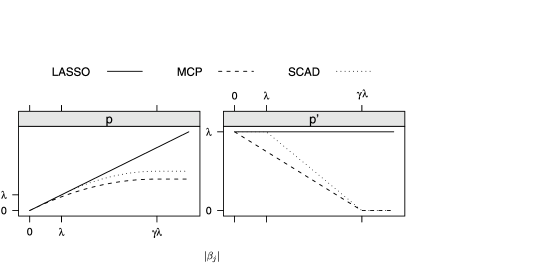
Figure 1: Shapes of the lasso, SCAD and MCP penalty functions. The panel on the left plots the penalties themselves, whereas the panel on the right plots the derivative of the penalty. Note that none of the penalties are differentiable at $\beta_{j}=0$.

The rationale behind the MCP can also be understood by considering its univariate solution. Consider the simple linear regression of $\mathbf{y}$ upon $\mathbf{x}$, with unpenalized least squares solution $z=n^{-1}\mathbf{x}^{\prime}\mathbf{y}$ (recall that $\mathbf{x}$ has been standardized so that $\mathbf{x}^{\prime}\mathbf{x}=n$). For this simple linear regression problem, the MCP estimator has the following closed form:

$$\hat{\beta}=f_{\mathrm{MCP}}(z,\lambda,\gamma)=\cases{\displaystyle\frac{S(z,\lambda)}{1-1/\gamma},&\quad if $|z|\leq\gamma\lambda$,\cr z,&\quad if $|z|>\gamma\lambda$,}$$ (3)

where $S$ is the soft-thresholding operator [Donoho and Johnstone (1994)] defined for $\lambda\geq 0$ by

$$S(z,\lambda)=\cases{z-\lambda,&\quad if $z>\lambda$,\cr 0,&\quad if $|z|\leq\lambda$,\cr z+\lambda,&\quad if $z<-\lambda$.}$$ (4)

Noting that $S(z,\lambda)$ is the univariate solution to the lasso, we can observe by comparison that MCP scales the lasso solution back toward the unpenalized solution by an amount that depends on $\gamma$. As $\gamma\to\infty$, the MCP and lasso solutions are the same. As $\gamma\to 1$, the MCP solution becomes the hard thresholding estimate $zI_{|z|>\lambda}$. Thus, in the univariate sense, the MCP produces the “firm shrinkage” estimator of Gao and Bruce (1997).

In the special case of an orthonormal design matrix, subset selection is equivalent to hard-thresholding, the lasso is equivalent to soft-thresholding, and MCP is equivalent to firm-thresholding. Thus, the lasso may be thought of as performing a kind of multivariate soft-thresholding, subset selection as multivariate hard-thresholding, and the MCP as multivariate firm-thresholding.

The univariate solution of the MCP is employed by the coordinate descent algorithm to obtain the coordinate-wise minimizer of the objective function. In this setting, however, the role of the unpenalized solution is now played by the unpenalized regression of $\mathbf{x}_{j}$’s partial residuals on $\mathbf{x}_{j}$, and denoted $z_{j}$. Introducing the notation $-j$ to refer to the portion that remains after the $j$th column or element is removed, the partial residuals of $\mathbf{x}_{j}$ are $\mathbf{r}_{-j}=\mathbf{y}-\mathbf{X}_{-j}\bolds{\beta}_{-j}$, where $\bolds{\beta}_{-j}$ is the most recently updated value of $\bolds{\beta}$. Thus, at step $j$ of iteration $m$, the following three calculations are made:

• calculate

  $$z_{j}=n^{-1}\mathbf{x}_{j}^{\prime}\mathbf{r}_{-j}=n^{-1}\mathbf{x}_{j}^{\prime}\mathbf{r}+\beta_{j}^{(m)},$$

• update $\beta_{j}^{(m+1)}\leftarrow f_{\mathrm{MCP}}(z_{j},\lambda,\gamma)$,

• update $\mathbf{r}\leftarrow\mathbf{r}-(\beta_{j}^{(m+1)}-\beta_{j}^{(m)})\mathbf{x}_{j}$,

where the last step ensures that $\mathbf{r}$ always holds the current values of the residuals. Note that $z_{j}$ can be obtained by regressing $\mathbf{x}_{j}$ on either the partial residuals or the current residuals; using the current residuals is more computationally efficient, however, as it does not require recalculating partial residuals for each update.

2.2 SCAD

The SCAD penalty Fan and Li (2001) defined on $[0,\infty)$ is given by

$$p_{\lambda,\gamma}(\theta) = \cases{\lambda\theta,&\quad if $\theta\leq\lambda$,\cr\displaystyle\frac{\gamma\lambda\theta-0.5(\theta^{2}+\lambda^{2})}{\gamma-1},&\quad if $\lambda<\theta\leq\gamma\lambda$,\cr\displaystyle\frac{\lambda^{2}(\gamma^{2}-1)}{2(\gamma-1)},&\quad if $\theta>\gamma\lambda$,}$$

$$p_{\lambda}^{\prime}(\theta) = \cases{\lambda,&\quad if $\theta\leq\lambda$,\cr\displaystyle\frac{\gamma\lambda-\theta}{\gamma-1},&\quad if $\lambda<\theta\leq\gamma\lambda$,\cr 0,&\quad if $\theta>\gamma\lambda$}$$

for $\lambda\geq 0$ and $\gamma>2$. The rationale behind the penalty is similar to that of MCP. Both penalties begin by applying the same rate of penalization as the lasso, and reduce that rate to 0 as $\theta$ gets further away from zero; the difference is in the way that they make the transition. The SCAD penalty is also illustrated in Figure 1.

The univariate solution for a SCAD-penalized regression coefficient is as follows, where again $z$ is the unpenalized linear regression solution:

$$\hat{\beta}=f_{\mathrm{SCAD}}(z,\lambda,\gamma)=\cases{S(z,\lambda),&\quad if $|z|\leq 2\lambda$,\cr\displaystyle\frac{S(z,\gamma\lambda/({\gamma-1}))}{1-1/(\gamma-1)},&\quad if $2\lambda<|z|\leq\gamma\lambda$,\cr z,&\quad if $|z|>\gamma\lambda$.}$$ (6)

This solution is similar to, although not the same as, the MCP solution/firm shrinkage estimator. Both penalties rescale the soft-thresholding solution toward the unpenalized solution. However, although SCAD has soft-thresholding as the limiting case when $\gamma\to\infty$, it does not have hard thresholding as the limiting case when $\gamma\to 2$. This univariate solution plays the same role in the coordinate descent algorithm for SCAD as $f_{\mathrm{MCP}}(z_{j},\lambda,\gamma)$ played for MCP.

2.3 Convergence

We now consider the convergence of coordinate descent algorithms for SCAD and MCP. We begin with the following lemma.

Lemma 1

Let $Q_{j,\lambda,\gamma}(\beta)$ denote the objective function $Q$, defined in (1), as a function of the single variable $\beta_{j}$, with the remaining elements of $\bolds{\beta}$ fixed. For the SCAD penalty with $\gamma>2$ and for the MCP with $\gamma>1$, $Q_{j,\lambda,\gamma}(\beta)$ is a convex function of $\beta_{j}$ for all $j$.

From this lemma, we can establish the following convergence properties of coordinate descent algorithms for SCAD and MCP.

Proposition 1

Let $\{\bolds{\beta}^{(k)}\}$ denote the sequence of coefficients produced at each iteration of the coordinate descent algorithms for SCAD and MCP. For all $k=0,1,2,\ldots,$

$$Q_{\lambda,\gamma}\bigl{(}\bolds{\beta}^{(k+1)}\bigr{)}\leq Q_{\lambda,\gamma}\bigl{(}\bolds{\beta}^{(k)}\bigr{)}.$$

Furthermore, the sequence is guaranteed to converge to a point that is both a local minimum and a global coordinate-wise minimum of $Q_{\lambda,\gamma}$.

Because the penalty functions of SCAD and MCP are not convex, neither the coordinate descent algorithms proposed here nor the LLA algorithm are guaranteed to converge to a global minimum in general. However, it is possible for the objective function $Q$ to be convex with respect to $\bolds{\beta}$ even though it contains a nonconvex penalty component. In particular, letting $c_{*}$ denote the minimum eigenvalue of $n^{-1}\mathbf{X}^{\prime}\mathbf{X}$, the MCP objective function is convex if $\gamma>1/c_{*}$, while the SCAD objective function is convex if $\gamma>1+1/c_{*}$ [Zhang (2010)]. If this is the case, then the coordinate descent algorithms converge to the global minimum. Section 4 discusses this issue further with respect to high-dimensional settings.

2.4 Pathwise optimization and initial values

Usually, we are interested in obtaining $\hat{\bolds{\beta}}$ not just for a single value of $\lambda$, but for a range of values extending from a maximum value $\lambda_{\max}$ for which all penalized coefficients are 0 down to $\lambda=0$ or to a minimum value $\lambda_{\min}$ at which the model becomes excessively large or ceases to be identifiable. When the objective function is strictly convex, the estimated coefficients vary continuously with $\lambda\in[\lambda_{\min},\ \lambda_{\max}]$ and produce a path of solutions regularized by $\lambda$. Examples of such paths may be seen in Figures 2 and 5.

Because the coefficient paths are continuous (under strictly convex objective functions), a reasonable approach to choosing initial values is to start at one extreme of the path and use the estimate $\hat{\bolds{\beta}}$ from the previous value of $\lambda$ as the initial value for the next value of $\lambda$. For MCP and SCAD, we can easily determine $\lambda_{\max}$, the smallest value for which all penalized coefficients are 0. From (3) and (6), it is clear that $\lambda_{\max}=z_{\max}$, where $z_{\max}=\max_{j}\{n^{-1}\mathbf{x}_{j}^{\prime}\mathbf{y}\}$ [for logistic regression (Section 3) $\lambda_{\max}$ is again equal to ${\max}_{j}\{z_{j}\}$, albeit with $z_{j}$ as defined in (10) and the quadratic approximation taken with respect to the intercept-only model]. Thus, by starting at $\lambda_{\max}$ with $\bolds{\beta}^{(0)}=\mathbf{0}$ and proceeding toward $\lambda_{\min}$, we can ensure that the initial values will never be far from the solution.

For all the numerical results in this paper, we follow the approach of Friedman, Hastie and Tibshirani (2010) and compute solutions along a grid of 100 $\lambda$ values that are equally spaced on the log scale.

3 Logistic regression with nonconvex penalties

For logistic regression, it is not possible to eliminate the need for an intercept by centering the response variable. For logistic regression, then, $\mathbf{y}$ will denote the original vector of 0–1 responses. Correspondingly, although $\mathbf{X}$ is still standardized, it now contains an unpenalized column of 1’s for the intercept, with corresponding coefficient $\beta_{0}$. The expected value of $\mathbf{y}$ once again depends on the linear function $\bolds{\eta}=\mathbf{X}\bolds{\beta}$, although the model is now

$$P(y_{i}=1|x_{i1},\ldots,x_{ip})=\pi_{i}=\frac{e^{\eta_{i}}}{1+e^{\eta_{i}}}.$$ (7)

Estimation of the coefficients is now accomplished via minimization of the objective function

$$\qquad Q_{\lambda,\gamma}(\bolds{\beta})=-\frac{1}{n}\sum_{i=1}^{n}\{y_{i}\log{\pi_{i}}+(1-y_{i})\log{(1-\pi_{i})}\}+\sum_{j=1}^{p}p_{\lambda,\gamma}(|\beta_{j}|).$$ (8)

Minimization can be approached by first obtaining a quadratic approximation to the loss function based on a Taylor series expansion about the value of the regression coefficients at the beginning of the current iteration, $\bolds{\beta}^{(m)}$. Doing so results in the familiar form of the iteratively reweighted least squares algorithm commonly used to fit generalized linear models [McCullagh and Nelder (1989)]:

$$Q_{\lambda,\gamma}(\bolds{\beta})\approx\frac{1}{2n}(\tilde{\mathbf{y}}-\mathbf{X}\bolds{\beta})^{\prime}\mathbf{W}(\tilde{\mathbf{y}}-\mathbf{X}\bolds{\beta})+\sum_{j=1}^{p}p_{\lambda,\gamma}(|\beta_{j}|),$$ (9)

where $\tilde{\mathbf{y}}$, the working response, is defined by

$$\tilde{\mathbf{y}}=\mathbf{X}\bolds{\beta}^{(m)}+\mathbf{W}^{-1}(\mathbf{y}-\bolds{\pi})$$

and $\mathbf{W}$ is a diagonal matrix of weights, with elements

$$w_{i}=\pi_{i}(1-\pi_{i}),$$

and $\bolds{\pi}$ is evaluated at $\bolds{\beta}^{(m)}$. We focus on logistic regression here, but the same approach could be applied to fit penalized versions of any generalized linear model, provided that the quantities $\tilde{\mathbf{y}}$ and $\mathbf{W}$ [as well as the residuals $\mathbf{r}\equiv\tilde{\mathbf{y}}-\mathbf{X}\bolds{\beta}^{(m)}$, which depend on $\tilde{\mathbf{y}}$ implicitly] are replaced with expressions specific to the particular response distribution and link function.

With this representation, the local linear approximation (LLA) and coordinate descent (CD) algorithms can be extended to logistic regression in a rather straightforward manner. At iteration $m$, the following two steps are taken:

Approximate the loss function based on $\bolds{\beta}^{(m)}$.

Execute one iteration of the LLA/CD algorithm, obtaining $\bolds{\beta}^{(m+1)}$. These two steps are then iterated until convergence for each value of $\lambda$. Note that for the coordinate descent algorithm, step (2) loops over all the covariates. Note also that step 2 must now involve the updating of the intercept term, which may be accomplished without modification of the underlying framework by setting $\lambda=0$ for the intercept term.

The local linear approximation is extended in a straightforward manner to reweighted least squares by distributing $\mathbf{W}$, obtaining the transformed covariates and response variable $\mathbf{W}^{1/2}\mathbf{X}$ and $\mathbf{W}^{1/2}\tilde{\mathbf{y}}$, respectively. The implications for coordinate descent algorithms are discussed in the next section.

Briefly, we note that, as is the case for the traditional iteratively reweighted least squares algorithm applied to generalized linear models, neither algorithm (LLA/CD) is guaranteed to converge for logistic regression. However, provided that adequate safeguards are in place to protect against model saturation, we have not observed failure to converge to be a problem for either algorithm.

3.1 Fixed scale solution

The presence of observation weights changes the form of the coordinate-wise updates. Let $v_{j}=n^{-1}\mathbf{x}_{j}^{\prime}\mathbf{W}\mathbf{x}_{j}$, and redefine $\mathbf{r}=\mathbf{W}^{-1}(\mathbf{y}-\bolds{\pi})$ and

$$z_{j} = \frac{1}{n}\mathbf{x}_{j}^{\prime}\mathbf{W}(\tilde{\mathbf{y}}-\mathbf{X}_{-j}\bolds{\beta}_{-j})$$ (10)

$$= \frac{1}{n}\mathbf{x}_{j}^{\prime}\mathbf{W}\mathbf{r}+v_{j}\beta_{j}^{(m)}.$$ (11)

Now, the coordinate-descent update for MCP is

$$\beta_{j}\leftarrow\cases{\displaystyle\frac{S(z_{j},\lambda)}{v_{j}-1/\gamma},&\quad if $|z_{j}|\leq v_{j}\gamma\lambda$,\cr\displaystyle\frac{z_{j}}{v_{j}},&\quad if $|z_{j}|>v_{j}\gamma\lambda$}$$ (12)

for $\gamma>1/v_{j}$ and for SCAD,

$$\beta_{j}\leftarrow\cases{\displaystyle\frac{S(z_{j},\lambda)}{v_{j}},&\quad if $|z_{j}|\leq\lambda(v_{j}+1)$,\cr\displaystyle\frac{S(z_{j},\gamma\lambda/(\gamma-1))}{v_{j}-1/(\gamma-1)},&\quad if $\lambda(v_{j}+1)<|z_{j}|\leq v_{j}\gamma\lambda$,\cr\displaystyle\frac{z_{j}}{v_{j}},&\quad if $|z_{j}|>v_{j}\gamma\lambda$}$$ (13)

for $\gamma>1+1/v_{j}$. Updating of $\mathbf{r}$ proceeds as in the linear regression case.

As is evident from comparing (3)/(6) with (12)/(13), portions of both numerator and denominator are being reweighted in logistic regression. In comparison, for linear regression, $v_{j}$ is always equal to 1 and this term drops out of the solution.

This reweighting, however, introduces some difficulties with respect to the choice and interpretation of the $\gamma$ parameter. In linear regression, the scaling factor by which solutions are adjusted toward their unpenalized solution is a constant [$1-1/\gamma$ for MCP, $1-1/(\gamma-1)$ for SCAD] for all values of $\lambda$ and for each covariate. Furthermore, for standardized covariates, this constant has a universal interpretation for all linear regression problems, meaning that theoretical arguments and numerical simulations investigating $\gamma$ do not need to be rescaled and reinterpreted in the context of applied problems.

In logistic regression, however, this scaling factor is constantly changing, and is different for each covariate. This makes choosing an appropriate value for $\gamma$ difficult in applied settings and robs the parameter of a consistent interpretation.

To illustrate the consequences of this issue, consider an attempt to perform logistic regression updates using $\gamma=3.7$, the value suggested for linear regression in Fan and Li (2001). Because $w_{i}$ cannot exceed 0.25, $\gamma$ cannot exceed $1/v_{j}$ and the solution is discontinuous and unstable. Note that this problem does not arise from the use of any particular algorithm—it is a direct consequence of the poorly behaved objective function with this value of $\gamma$.

3.2 Adaptive rescaling

To resolve these difficulties, we propose an adaptive rescaling of the penalty parameter $\gamma$ to match the continually changing scale of the covariates. This can be accomplished by simply replacing $p_{\lambda,\gamma}(|\beta_{j}|)$ with $p_{\lambda,\gamma}(|v_{j}\beta_{j}|)$. The algorithmic consequences for the LLA algorithm are straightforward. For coordinate descent, the updating steps become simple extensions of the linear regression solutions:

$$\beta_{j}\leftarrow\frac{f(z_{j},\lambda,\gamma)}{v_{j}}.$$

Note that, for MCP,

$$\frac{S(z_{j},\lambda)}{v_{j}(1-1/\gamma)}=\frac{S(z_{j},\lambda)}{v_{j}-1/\gamma^{*}},$$

where $\gamma^{*}=\gamma/v_{j}$. Thus, the adaptively rescaled solution is still minimizing the objective function (9), albeit with an alternate set of shape parameters $\{\gamma_{j}^{*}\}$ that are unknown until convergence is attained.

Note that rescaling by $v_{j}$ does not affect the magnitude of the penalty ($\lambda$), only the range over which the penalty is applied ($\gamma$). Is it logical to apply different scales to different variables? Keep in mind that, since $\mathbf{x}_{j}^{\prime}\mathbf{x}_{j}=n$ for all $j$, the rescaling factor $v_{j}$ will tend to be quite similar for all covariates. However, consider the case where a covariate is predominantly associated with observations for which $\hat{\pi}_{i}$ is close to 0 or 1. For such a covariate, adaptive rescaling will extend the range over which the penalization is applied. This seems to be a reasonable course of action, as large changes in this coefficient produce only small changes in the model’s fit, and provide less compelling evidence of a covariate’s importance.

SCAD does not have the property that its adaptively rescaled solution is equal to a solution of the regular SCAD objective function with different shape parameters. This is due to the fact that the scale of the penalty is tied to the scale of the coefficient by the $\theta<\lambda$ clause. One could make this clause more flexible by reparameterizing SCAD so that $p^{\prime}(\theta)=\lambda$ in the region $\theta<\gamma_{2}\lambda$, where $\gamma_{2}$ would be an additional tuning parameter. In this generalized case, adaptively rescaled SCAD would minimize a version of the original objective function in which the $\gamma$ parameters are rescaled by $v_{j}$, as in the MCP case.

As we will see in Section 5, this adaptive rescaling increases interpretability and makes it easier to select $\gamma$.

4 Convexity, stability and selection of tuning parameters

4.1 Convexity and stability

As mentioned in Section 2.3, the MCP/SCAD-penalized linear regression objective function is convex provided that $\gamma>1/c_{*}$ (MCP) or $\gamma>1+1/c_{*}$ (SCAD). This result can be extended to logistic regression as well via the following proposition.

Proposition 2

Let $c_{*}(\bolds{\beta})$ denote the minimum eigenvalue of $n^{-1}\mathbf{X}^{\prime}\mathbf{W}\mathbf{X}$, where $\mathbf{W}$ is evaluated at $\bolds{\beta}$. Then the objective function defined in (8) is a convex function of $\bolds{\beta}$ on the region where $c_{*}(\bolds{\beta})>1/\gamma$ for MCP, and where $c_{*}(\bolds{\beta})>1/(\gamma-1)$ for SCAD.

A convex objective function is desirable for (at least) two reasons. First, for any algorithm (such as coordinate descent) which converges to a critical point of the objective function, convexity ensures that the algorithm converges to the unique global minimum. Second, convexity ensures that $\hat{\bolds{\beta}}$ is continuous with respect to $\lambda$, which in turn ensures good initial values for the scheme described in Section 2.4, thereby reducing the number of iterations required by the algorithm.

There are obvious practical benefits to using an algorithm that converges rapidly to the unique global solution. However, convexity may also be desirable from a statistical perspective. In the absence of convexity, $\hat{\bolds{\beta}}$ is not necessarily continuous with respect to the data—that is, a small change in the data may produce a large change in the estimate. Such estimators tend to have high variance [Breiman (1996); Bruce and Gao (1996)] in addition to being unattractive from a logical perspective. Furthermore, discontinuity with respect to $\lambda$ increases the difficulty of choosing a good value for the regularization parameter.

4.2 Local convexity diagnostics

However, it is not always necessary to attain global convexity. In high-dimensional settings where $p>n$, global convexity is neither possible nor relevant. In such settings, sparse solutions for which the number of nonzero coefficients is much lower than $p$ are desired. Provided that the objective function is convex in the local region that contains these sparse solutions, we will still have stable estimates and smooth coefficient paths in the parameter space of interest.

Of considerable practical interest, then, is a diagnostic that would indicate, for nonconvex penalties such as SCAD and MCP, which regions of the coefficient paths are locally convex and which are not. Here, we introduce a definition for local convexity and a diagnostic measure which can be easily computed from the data and which can indicate which regions of the coefficient paths retain the benefits of convexity and which do not.

Recall the conditions for global convexity: $\gamma$ must be greater than $1/c_{*}$ for MCP ($1+1/c_{*}$ for SCAD), where $c_{*}$ denoted the minimum eigenvalue of $n^{-1}\mathbf{X}^{\prime}\mathbf{X}$. We propose modifying this cutoff so that only the covariates with nonzero coefficients (the covariates which are “active” in the model) are included in the calculation of $c_{*}$. Note that neither $\gamma$ nor $\mathbf{X}$ change with $\lambda$. What does vary with $\lambda$ is set of active covariates; generally speaking, this will increase as $\lambda$ decreases (with correlated/collinear data, however, exceptions are possible). Thus, local convexity of the objective function will not be an issue for large $\lambda$, but may cease to hold as $\lambda$ is lowered past some critical value $\lambda^{*}$.

Specifically, let $\hat{\bolds{\beta}}(\lambda)$ denote the minimizer of (1) for a certain value of $\lambda$, $A(\lambda)=\{j\dvtx\hat{\beta}_{j}(\lambda)\neq 0\}$ denote the active set of covariates, $U(\lambda)=A(\lambda)\cup A(\lambda^{-})$ denote the set of covariates that are either currently active given a value $\lambda$ or that will become active imminently upon the lowering of $\lambda$ by an infinitesimal amount, and let $\mathbf{X}_{U}(\lambda)$ denote the design matrix formed from only those covariates for which $j\in U(\lambda)$, with $c_{*}(\lambda)$ denoting the minimum eigenvalue of $n^{-1}{\mathbf{X}_{U(\lambda)}}^{\prime}\mathbf{X}_{U(\lambda)}$. Now, letting

$$\lambda^{*}=\inf\{\lambda\dvtx\gamma>1/c_{*}(\lambda)\}\qquad\mbox{for MCP}\hskip 25.5pt$$

and

$$\lambda^{*}=\inf\{\lambda\dvtx\gamma>1+1/c_{*}(\lambda)\}\qquad\mbox{for SCAD,}$$

we define the $\lambda$ interval over which the objective function is “locally convex” to be $(\infty,\lambda^{*})$. Correspondingly, the objective function is locally nonconvex (and globally nonconvex) in the region $[\lambda^{*},0]$. Because $c_{*}(\lambda)$ changes only when the composition of $U(\lambda)$ changes, it is clear that $\lambda^{*}$ must be a value of $\lambda$ for which $A(\lambda)\neq A(\lambda^{-})$.

For logistic regression, let $c_{*}(\lambda)$ represent the minimum eigenvalue of $n^{-1}{\mathbf{X}_{U(\lambda)}}^{\prime}\mathbf{W}\mathbf{X}_{U(\lambda)}-\mathbf{D}_{p}$, where $\mathbf{W}$ is evaluated at $\hat{\bolds{\beta}}(\lambda)$ and $\mathbf{D}_{p}$ is a diagonal matrix that depends on the penalty function. For the fixed scale estimation of Section 3.1, $\mathbf{D}_{p}$ has elements $\{1/\gamma\}$ for MCP and $\{1/(\gamma-1)\}$ for SCAD, while for the adaptively rescaled estimation of Section 3.2, $\mathbf{D}_{p}$ has elements $\{n^{-1}\mathbf{x}_{k}^{\prime}\mathbf{W}\mathbf{x}_{k}/\gamma\}$ for MCP and $\{n^{-1}\mathbf{x}_{k}^{\prime}\mathbf{W}\mathbf{x}_{k}/(\gamma-1)\}$ for SCAD. For $c_{*}(\lambda)$ defined in this manner, $\lambda^{*}$ equals the smallest value of $\lambda$ such that $c_{*}(\lambda)>0$.

Figure 2: Example MCP coefficient paths for simulated data where $p>n$. The shaded region is the region in which the objective function is not locally convex. Note that the solutions are continuous and stable in the locally convex regions, but discontinuous and erratic otherwise.

The practical benefit of these diagnostics can be seen in Figure 2, which depicts examples of coefficient paths from simulated data in which $n=20$ and $p=50$. As is readily apparent, solutions are smooth and well behaved in the unshaded, locally convex region, but discontinuous and noisy in the shaded region which lies to the right of $\lambda^{*}$. Figure 2 contains only MCP paths; the corresponding figures for SCAD paths look very similar. Figure 2 displays linear regression paths; paths for logistic regression can be seen in Figure 5.

The noisy solutions in the shaded region of Figure 2 may arise from numerical convergence to suboptimal solutions, inherent statistical variability arising from minimization of a nonconvex function, or a combination of both; either way, however, the figure makes a compelling argument that practitioners of regression methods involving nonconvex penalties should know which region their solution resides in.

4.3 Selection of $\gamma$ and $\lambda$

Estimation using MCP and SCAD models depends on the choice of the tuning parameters $\gamma$ and $\lambda$. This is usually accomplished with cross-validation or using an information criterion such as AIC or BIC. Each approach has its shortcomings.

Information criteria derived using asymptotic arguments for unpenalized regression models are on questionable ground when applied to penalized regression problems where $p>n$. Furthermore, defining the number of parameters in models with penalization and shrinkage present is complicated and affects lasso, MCP and SCAD differently. Finally, we have observed that AIC and BIC have a tendency, in some settings, to select local mimima in the nonconvex region of the objective function.

Cross-validation does not suffer from these issues; on the other hand, it is computationally intensive, particularly when performed over a two-dimensional grid of values for $\gamma$ and $\lambda$, some of which may not possess convex objective functions and, as a result, converge slowly. This places a barrier in the way of examining the choice of $\gamma$, and may lead practitioners to use default values that are not appropriate in the context of a particular problem.

It is desirable to select a value of $\gamma$ that produces parsimonious models while avoiding the aforementioned pitfalls of nonconvexity. Thus, we suggest the following hybrid approach, using BIC, cross-validation and convexity diagnostics in combination, which we have observed to work well in practice. For a path of solutions with a given value of $\gamma$, use AIC/BIC to select $\lambda$ and use the aforementioned convexity diagnostics to determine the locally convex regions of the solution path. If the chosen solution lies in the region below $\lambda^{*}$, increase $\gamma$ to make the penalty more convex. On the other hand, if the chosen solution lies well above $\lambda^{*}$, one can lower $\gamma$ without fear of nonconvexity. Once this process has been iterated a few times to find a value of $\gamma$ that seems to produce an appropriate balance between parsimony and convexity, use cross-validation to choose $\lambda$ for this value of $\gamma$. This approach is illustrated in Section 6.

5 Numerical results

5.1 Computational efficiency

In this section we assess the computational efficiency of the coordinate descent and LLA algorithms for fitting MCP and SCAD regression models. We examine the time required to fit the entire coefficient path for linear and logistic regression models.

In these simulations, the response for linear regression was generated from the standard normal distribution, while for logistic regression, the response was generated as a Bernoulli random variable with $P(y_{i}=1)=0.5$ for all $i$.

To investigate whether or not the coordinate descent algorithm experiences difficulty in the presence of correlated predictors, covariate values were generated in one of two ways: independently from the standard normal distribution (i.e., no correlation between the covariates), and from a multivariate normal distribution with a pairwise correlation of $\rho=0.9$ between all covariates.

To ensure that the comparison between the algorithms was fair and not unduly influenced by failures to converge brought on by nonconvexity or model saturation, $n$ was chosen to equal 1000 and $\gamma$ was set equal to $1/c_{*}$, thereby ensuring a convex objective function for linear regression. This does not necessarily ensure that the logistic regression objective function is convex, although with adaptive rescaling, it works reasonably well. In all of the cases investigated, the LLA and coordinate descent algorithms converged to the same path (within the accuracy of the convergence criteria). The median times required to fit the entire coefficient path are presented as a function of $p$ in Figure 3.

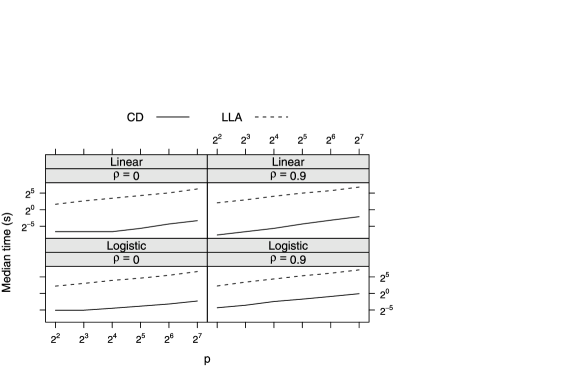
Figure 3: Time required (in seconds) to fit the entire coefficient paths for linear and logistic regression, employing either the local linear approximation (LLA) algorithm or the coordinate descent (CD) algorithm. Both axes are on the log scale. Times displayed are averaged over 100 independently generated data sets. The coordinate descent algorithm is at least 100 times faster than the LLA algorithm at all points.

Interestingly, the slope of both lines in Figure 3 is close to 1 in each setting (on the log scale), implying that both coordinate descent and LLA exhibit a linear increase in computational burden with respect to $p$ over the range of $p$ investigated here. However, coordinate descent algorithm is drastically more efficient—up to 1000 times faster. The coordinate descent algorithm is somewhat (2–5 times) slower in the presence of highly correlated covariates, although it is still at least 100 times faster than LLA in all settings investigated.

5.2 Comparison of MCP, SCAD and lasso

We now turn our attention to the statistical properties of MCP and SCAD in comparison with the lasso. We will examine two instructive sets of simulations, comparing these nonconvex penalty methods to the lasso. The first set is a simple series designed to illustrate the primary differences between the methods. The second set is more complex, and designed to mimic the applications to real data in Section 6.

In the simple settings, covariate values were generated independently from the standard normal distribution. The sample sizes were $n=100$ for linear regression and $n=400$ for logistic regression. In the complex settings, the design matrices from the actual data sets were used.

For each data set, the MCP and SCAD coefficient paths were fit using the coordinate descent algorithm described in this paper, and lasso paths were fit using the glmnet package [Friedman, Hastie and Tibshirani (2010)]. Tenfold cross-validation was used to choose $\lambda$.

Setting 1. We begin with a collection of simple models in which there are four nonzero coefficients, two of which equal to $+s$, the other two equal to $-s$. Given these values of the coefficient vector, responses were generated from the normal distribution with mean $\eta_{i}$ and variance 1 for linear regression, and for logistic regression, responses were generated according to (7).

For the simulations in this setting, we used the single value $\gamma=3$ in order to illustrate that reasonable results can be obtained without investigation of the tuning parameter if adaptive rescaling is used for penalized logistic regression. Presumably, the performance of both MCP and SCAD would be improved if $\gamma$ was chosen in a more careful manner, tailored to each setting; nevertheless, the simulations succeed in demonstrating the primary statistical differences between the methods.

We investigate the estimation efficiency of MCP, SCAD and lasso as $s$ and $p$ are varied. These results are shown in Figure 4.

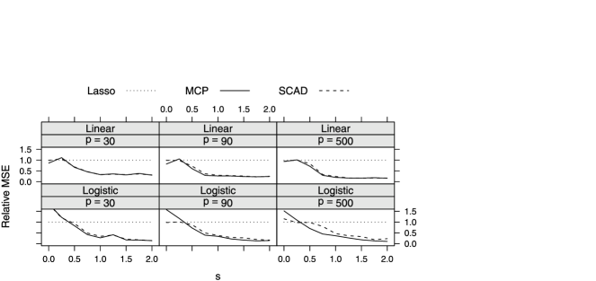
Figure 4: Relative (to the lasso) mean squared error for MCP- and SCAD-penalized linear and logistic regression. MSE was calculated for each penalty on 100 independently generated data sets, and the ratio of the medians is plotted. MCP and SCAD greatly outperform lasso for large coefficients, but not necessarily for small coefficients.

Figure 4 illustrates the primary difference between MCP/SCAD and lasso. MCP and SCAD are more aggressive modeling strategies, in the sense that they allow coefficients to take on large values much more easily than lasso. As a result, they are capable of greatly outperforming the lasso when large coefficients are present in the underlying model. However, the shrinkage applied by the lasso is beneficial when coefficients are small, as seen in the regions of Figure 4 in which $s$ is near zero. In such settings, MCP and SCAD are more likely to overfit the noisy data. This is true for both linear and logistic regression. This tendency is worse for logistic regression than it is for linear regression, worse for MCP than it is for SCAD, and worse when $\gamma$ is closer to 1 (results supporting this final comparison not shown).

Setting 2. In this setting we examine the performance of MCP, SCAD and lasso for the kinds of design matrices often seen in biomedical applications, where covariates contain complicated patterns of correlation and high levels of multicollinearity. Section 6 describes in greater detail the two data sets, which we will refer to here as “Genetic Association” and “Microarray,” but it is worth noting here that for the Genetic Association case, $n=800$ and $p=532$, while for the Microarray case, $n=38$ and $p=7129$.

In both simulations the design matrix was held constant while the coefficient and response vectors changed from replication to replication. In the Genetic Association case, 5 coefficient values were randomly generated from the exponential distribution with rate parameter 3, given a random ($+/-$) sign, and randomly assigned to one of the 532 SNPs (the rest of the coefficients were zero). In the Microarray case, 100 coefficient values were randomly generated from the normal distribution with mean 0 and standard deviation 3, and randomly assigned among the 7129 features. Once the coefficient vectors were generated, responses were generated according to (7). This was repeated 500 times for each case, and the results are displayed in Table 1.

=260pt Misclassification Penalty error (%) Model size Correct (%) Genetic association    MCP ($\gamma=1.5$) 38.7 02.1 54.7    SCAD ($\gamma=2.5$) 38.7 09.5 25.0    Lasso 38.8 12.6 20.6 Microarray    MCP ($\gamma=5$) 19.7 04.3 03.2    MCP ($\gamma=20$) 16.7 07.5 04.3    SCAD ($\gamma=20$) 16.4 08.7 04.3    Lasso 16.2 08.8 04.3

Table 1: Simulation results: Setting 2% correct refers to the percent of variables selected by the model that had nonzero coefficients in the generating model

The Genetic Association simulation—reflecting the presumed underlying biology in these kinds of studies—was designed to be quite sparse. We expected the more sparse MCP method to outperform the lasso here, and it does. All methods achieve similar predictive accuracy, but MCP does so using far fewer variables and with a much lower percentage of spurious covariates in the model.

The Microarray simulation was designed to be unfavorable to sparse modeling—a large number of nonzero coefficients, many of which are close to zero. As is further discussed in Section 6, $\gamma$ should be large in this case; when $\gamma=5$, MCP produces models with diminished accuracy in terms of both prediction and variable selection. However, it is not the case that lasso is clearly superior to MCP here; if $\gamma$ is chosen appropriately, the predictive accuracy of the lasso can be retained, with gains in parsimony, by applying MCP with $\gamma=20$.

In the microarray simulation, the percentage of variables selected that have a nonzero coefficient in the generating model is quite low for all methods. This is largely due to high correlation among the features. The methods achieve good predictive accuracy by finding predictors that are highly correlated with true covariates, but are unable to distinguish the causative factors from the rest in the network of interdependent gene expression levels. This is not an impediment for screening and diagnostic applications, although it may or may not be helpful for elucidating the pathway of disease.

SCAD, the design of which has similarities to both MCP and lasso, lies in between the two methodologies. However, in these two cases, SCAD is more similar to lasso than it is to MCP.

6 Applications

6.1 Genetic association

Genetic association studies have become a widely used tool for detecting links between genetic markers and diseases. The example that we will consider here involves data from a case-control study of age-related macular degeneration consisting of 400 cases and 400 controls. We confine our analysis to 30 genes that previous biological studies have suggested may be related to the disease. These genes contained 532 markers with acceptably high call rates and minor allele frequencies. Logistic regression models penalized by lasso, SCAD and MCP were fit to the data assuming an additive effect for all markers (i.e., for a homozygous dominant marker, $x_{ij}=2$, for a heterozygous marker, $x_{ij}=1$, and for a homozygous recessive marker, $x_{ij}=0$). As an illustration of computational savings in a practical setting, the LLA algorithm required 17 minutes to produce a single MCP path of solutions, as compared to 2.5 seconds for coordinate descent.

As described in Section 4.3, we used BIC and convexity diagnostics to choose an appropriate value of $\gamma$; this is illustrated in the top half of Figure 5. The biological expectation is that few markers are associated with the disease; this is observed empirically as well, as a low value of $\gamma=1.5$ was observed to balance sparsity and convexity in this setting. In a similar fashion, $\gamma=2.5$ was chosen for SCAD.

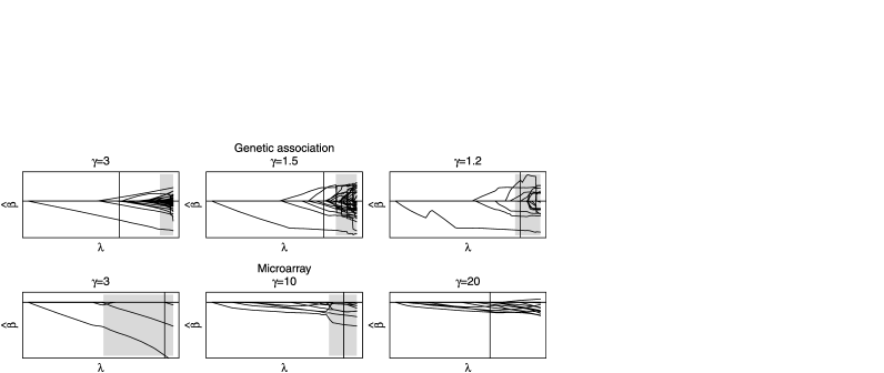
Figure 5: MCP coefficient paths for various values of $\gamma$ for the two studies of Section 6. The shaded region depicts areas that are not locally convex, and a vertical line is drawn at the value of $\lambda$ selected by BIC. For the sparse genetic association data, small values of $\gamma$ produce the best fit; for the dense microarray data, large values are preferred.

Ten-fold cross-validation was then used to choose $\lambda$ for MCP, SCAD and lasso. The number of parameters in the selected model, along with the corresponding cross-validation errors, are listed in Table 2. The results indicate that MCP is better suited to handle this sparse regression problem than either SCAD or lasso, achieving a modest reduction in cross-validated prediction error while producing a much more sparse model. As one would expect, the SCAD results are in between MCP and lasso.

Table 2: Genetic association results

Penalty	Model size	CV error (%)
MCP	007	39.4
SCAD	025	40.6
Lasso	103	40.9

6.2 Gene expression

Next, we examine the gene expression study of leukemia patients presented in Golub et al. (1999). In the study the expression levels of 7129 genes were recorded for 27 patients with acute lymphoblastic leukemia (ALL) and 11 patients with acute myeloid leukemia (AML). Expression levels for an additional 34 patients were measured and reserved as a test set. Logistic regression models penalized by lasso, SCAD and MCP were fit to the training data.

Biologically, this problem is more dense than the earlier application. Potentially, a large number of genes are affected by the two types of leukemia. In addition, the sample size is much smaller for this problem. These two factors suggest that a higher value of $\gamma$ is appropriate, an intuition borne out in Figure 5. The figure suggests that $\gamma\approx 20$ may be needed in order to obtain an adequately convex objective function for this problem (we used $\gamma=20$ for both MCP and SCAD).

With $\gamma$ so large, MCP and SCAD are quite similar to lasso; indeed, all three methods classify the test set observations in the same way, correctly classifying 31$/$34. Analyzing the same data, Park and Hastie (2007) find that lasso-penalized logistic regression is comparable with or more accurate than several other competing methods often applied to high-dimensional classification problems. The same would therefore apply to MCP and SCAD as well; however, MCP achieved its success using only 11 predictors, compared to 13 for lasso and SCAD. This is an important consideration for screening and diagnostic applications such as this one, where the goal is often to develop an accurate test using as few features as possible in order to control cost.

Note that, even in a problem such as this one with a sample size of 38 and a dozen features selected, there may still be an advantage to the sparsity of MCP and the parsimonious models it produces. To take advantage of MCP, however, it is essential to choose $\gamma$ wisely—using the value $\gamma=5$ (much too sparse for this problem) tripled the test error to 9$/$34. We are not aware of any method that can achieve prediction accuracy comparable to MCP while using only 11 features or fewer.

7 Discussion

The results from the simulation studies and data examples considered in this paper provide compelling evidence that nonconvex penalties like MCP and SCAD are worthwhile alternatives to the lasso in many applications. In particular, the numerical results suggest that MCP is often the preferred approach among the three methods.

Many researchers and practitioners have been reluctant to embrace these methods due to their lack of convexity, and for good reason: nonconvex objective functions are difficult to optimize and often produce unstable solutions. However, we provide here a fast, efficient and stable algorithm for fitting MCP and SCAD models, as well as introduce diagnostic measures to indicate which regions of a coefficient path are locally convex and which are not. Furthermore, we introduce an adaptive rescaling for logistic regression which makes selection of the tuning parameter $\gamma$ much easier and more intuitive. All of these innovations are publicly available as an open-source R package (http://cran.r-project.org) called ncvreg. We hope that these efforts remove some of the barriers to the further study and use of these methods in both research and practice.

Appendix

Although the objective functions under consideration in this paper are not differentiable, they possess directional derivatives and directional second derivatives at all points $\bolds{\beta}$ and in all directions $\mathbf{u}$ for $\bolds{\beta},\mathbf{u}\in\mathbb{R}^{p}$. We use $d_{\mathbf{u}}Q$ and $d_{\mathbf{u}}^{2}Q$ to represent the derivative and second derivative of $Q$ in the direction $\mathbf{u}$.

Proof of Lemma 1 For all $\beta_{j}\in(-\infty,\infty)$,

$$\min\{d_{-}^{2}Q_{j,\lambda,\gamma}(\beta),d_{+}^{2}Q_{j,\lambda,\gamma}(\beta)\}\geq\cases{\displaystyle 1-\frac{1}{\gamma}&\quad for MCP,\cr\displaystyle 1-\frac{1}{\gamma-1}&\quad for SCAD.}$$

Thus, $Q_{j,\lambda,\gamma}(\beta)$ is a strictly convex function on $(-\infty,\infty)$ if $\gamma>1$ for MCP and if $\gamma>2$ for SCAD.

Proof of Proposition 1 Tseng (2001) establishes sufficient conditions for the convergence of cyclic coordinate descent algorithms to coordinate-wise minima. The strict convexity in each coordinate direction established in Lemma 1 satisfies the conditions of Theorems 4.1 and 5.1 of that article. Because $Q$ is continuous, either theorem can be directly applied to demonstrate that the coordinate descent algorithms proposed in this paper converge to coordinate-wise minima. Furthermore, because all directional derivatives exist, every coordinate-wise minimum is also a local minimum.

Proof of Proposition 2 For all $\bolds{\beta}\in\mathbb{R}^{p}$,

$$\min\limits_{\mathbf{u}}\{d_{\mathbf{u}}^{2}Q_{\lambda,\gamma}(\bolds{\beta})\}\geq\cases{\displaystyle\frac{1}{n}\mathbf{X}^{\prime}\mathbf{W}\mathbf{X}-\frac{1}{\gamma}\mathbf{I}&\quad for MCP,\cr\displaystyle\frac{1}{n}\mathbf{X}^{\prime}\mathbf{W}\mathbf{X}-\frac{1}{\gamma-1}\mathbf{I}&\quad for SCAD.}$$

Thus, $Q_{\lambda,\gamma}(\bolds{\beta})$ is a convex function on the region for which $c_{*}(\bolds{\beta})>1/\gamma$ for MCP, and where $c_{*}(\bolds{\beta})>1/(\gamma-1)$ for SCAD.

References

- Breiman (1996) Breiman, L. (1996). Heuristics of instability and stabilization in model selection. Ann. Statist. 24 2350–2383. \MR1425957
- Bruce and Gao (1996) Bruce, A. G. and Gao, H. Y. (1996). Understanding WaveShrink: Variance and bias estimation. Biometrika 83 727–745. \MR1440040
- Donoho and Johnstone (1994) Donoho, D. L. and Johnstone, J. M. (1994). Ideal spatial adaptation by wavelet shrinkage. Biometrika 81 425–455. \MR1311089
- Efron et al. (2004) Efron, B., Hastie, T., Johnstone, I. and Tibshirani, R. (2004). Least angle regression. Ann. Statist. 32 407–451. \MR2060166
- Fan and Li (2001) Fan, J. and Li, R. (2001). Variable selection via nonconcave penalized likelihood and its oracle properties. J. Amer. Statist. Assoc. 96 1348–1361. \MR1946581
- Friedman, Hastie and Tibshirani (2010) Friedman, J., Hastie, T. and Tibshirani, R. (2010). Regularization paths for generalized linear models via coordinate descent. J. Statist. Softw. 33 1–22.
- Friedman et al. (2007) Friedman, J., Hastie, T., Höfling, H. and Tibshirani, R. (2007). Pathwise coordinate optimization. Ann. Appl. Statist. 1 302–332. \MR2415737
- Gao and Bruce (1997) Gao, H. Y. and Bruce, A. G. (1997). WaveShrink with firm shrinkage. Statist. Sinica 7 855–874. \MR1488646
- Golub et al. (1999) Golub, T. R., Slonim, D. K., Tamayo, P., Huard, C., Gaasenbeek, M., Mesirov, J. P., Coller, H., Loh, M. L., Downing, J. R., Caligiuri, M. A. et al. (1999). Molecular classification of cancer: Class discovery and class prediction by gene expression monitoring. Science 286 531–536.
- McCullagh and Nelder (1989) McCullagh, P. and Nelder, J. A. (1989). Generalized Linear Models. Chapman and Hall/CRC, Boca Raton, FL.
- Park and Hastie (2007) Park, M. Y. and Hastie, T. (2007). L1 regularization path algorithm for generalized linear models. J. Roy. Statist. Soc. Ser. B 69 659–677. \MR2370074
- Tibshirani (1996) Tibshirani, R. (1996). Regression shrinkage and selection via the lasso. J. Roy. Statist. Soc. Ser. B 58 267–288. \MR1379242
- Tseng (2001) Tseng, P. (2001). Convergence of a block coordinate descent method for nondifferentiable minimization. J. Optim. Theory Appl. 109 475–494. \MR1835069
- Wu and Lange (2008) Wu, T. T. and Lange, K. (2008). Coordinate descent algorithms for lasso penalized regression. Ann. Appl. Statist. 2 224–244. \MR2415601
- Yu et al. (2007) Yu, J., Yu, J., Almal, A. A., Dhanasekaran, S. M., Ghosh, D., Worzel, W. P. and Chinnaiyan, A. M. (2007). Feature selection and molecular classification of cancer using genetic programming. Neoplasia 9 292–303.
- Zhang (2010) Zhang, C. H. (2010). Nearly unbiased variable selection under minimax concave penalty. Ann. Statist. 38 894–942. \MR2604701
- Zou and Li (2008) Zou, H. and Li, R. (2008). One-step sparse estimates in nonconcave penalized likelihood models. Ann. Statist. 36 1509–1533. \MR2435443