Polarons in suspended carbon nanotubes

Abstract

We prove theoretically the possibility of electric-field controlled polaron formation involving flexural (bending) modes in suspended carbon nanotubes. Upon increasing the field, the ground state of the system with a single extra electron undergoes a first order phase transition between an extended state and a localized polaron state. For a common experimental setup, the threshold electric field is only of order $\simeq 10^{-2}$ V/$\mu$m.

Due to their unique material properies, carbon nanotubes make ideal flexible nano-rods for mechanical applications r1 . Coupling their mechanical motion to electronic degrees of freedom leads to non-linear dynamics r4 . Current technology r2 allows for the fabrication of ultra-clean nanotubes in which electrons propagate ballistically r1.5 rather than diffusively. In combination with a high quality factor r3 , this allows for resonant excitation and coherent manipulation of discrete degrees of freedom. The envisioned devices may find application in quantum information processing.

In current devices, a discrete spectrum is obtained by embedding a quantum dot on a suspended nanotube r4 ; r2 . In this paper we prove the possibility of the controlable formation of discrete states of a different kind, namely polarons. The setup is shown in Figure 1. It consists of an ultra-clean carbon nanotube cantilever. We consider a single wall semi-conducting nanotube. The setup is similar to the nano-relay proposed in Ref. r5, and to the experimental setup of Ref. r6, , but operated in a different regime, namely that of a single electron on the cantilever.

If the electron enters the suspended part of the tube, it experiences a force $\bm{F}=-{\rm e}\bm{E}$. The electric field $\bm{E}$ may be due to an external source, or to an induced image charge in the substrate below the cantilever. The force $\bm{F}$ deforms the tube. As a result, the potential energy of the electron is lowered. Thus the tube deformation produces a potential well that may trap the electron.

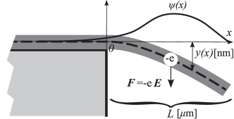
Figure 1: Setup: A single wall carbon nanotube cantilever of length $L$. The supported part of the tube rests on an insulating substrate. An electron that enters the suspended part of the tube experiences a force $\bm{F}=-{\rm e}\bm{E}$ perpendicular to the tube. As a result the tube is deformed so that each point $x$ on the tube undergoes a displacement $y(x)$ perpendicular to the $x$-axis. The electron wave function $\psi(x)$ is also indicated.

The trapping of an electron in a lattice deformation in a bulk solid is a well-studied topic r7 . The resulting quasi-particle is called a polaron. Previous studies of polarons in carbon nanotubes r8 considered only axial stretching and radial breathing modes of the tube, while our study concentrates on macroscopic flexural (bending) modes.

Our main results are contained in Fig. 3. At small electric fields, the ground state consists of an undeformed tube and an extended electron. As the field is increased beyond a critical value, the system undergoes a first order phase transition to a localized polaron state. For realistic values of a suspended tube length $L=1$ $\mu$m, and tube radius $r=1$ nm, the threshold electric field is $0.031$ V/$\mu$m and the tip deviation is $0.54$ nm. This is the field that would be produced by an image charge induced in a metallic substrate $0.10$ $\mu$m below the tube.

We start our analysis by noting that the typical energy scale for the polaron state is set by the electron confinement energy $\varepsilon_{e}=\hbar^{2}/2m^{*}L^{2}$, where $m^{*}$ is the effective electron mass. The ratio $\hbar\omega_{0}/\varepsilon_{e}$, where $\omega_{0}$ is the frequency of the lowest flexural mode of the tube, turns out to equal $0.09$, independent of $r$ or $L$. This ratio is small essentially because electrons weigh much less than carbon atoms. We therefore neglect the zero point motion (associated with energy $\hbar\omega_{0}$) of the cantilever and treat its displacement as a classical variable.

The supported part of the tube is tightly clamped to the substrate by van der Waals forces and cannot be deformed. We take the tube-element that was at $\bm{r}_{0}=x\,\hat{\bm{x}}$ to be displaced to $\bm{r}=x\,\hat{\bm{x}}+y(x)\,\hat{\bm{y}}$ under deformation. This is valid in the small deflection regime where ${\rm max}\{|y(x)|\}\ll L$. The system is described by two fields, namely, the tube profile $y(x)$ and the wave function $\psi(x)$ of the single electron in the conduction band. The boundary conditions on the tube profile are $y(x\leq 0)=y^{\prime}(x\leq 0)=0$ and $y^{\prime\prime}(L)=y^{\prime\prime\prime}(L)=0$. The boundary conditions on the wave function are $\psi(-\infty)=\psi(L)=0$. The wave function can be taken as real, and is normalized.

The ground state configuration is obtained by minimizing the energy functional

$$H[\psi,y]=\int_{-\infty}^{L}dx\,\underbrace{\frac{\hbar^{2}}{2m^{*}}\left(\partial_{x}\psi\right)^{2}}_{=T}+\underbrace{eEy\psi^{2}}_{=V}+\underbrace{\frac{YI}{2}\left(\partial_{x}^{2}y\right)^{2}}_{=U}.$$ (1)

The term $T$ is the kinetic energy of the electron. The effective mass $m^{*}$ is inversely proportional to the radius $r$ of the nanotube r9 . For zig-zag nanotubes $m^{*}=1.8\,m_{e}a_{0}/r$ where $m_{e}$ is the true electron mass and $a_{0}$ is the Bohr radius. For tubes with chiralities other than zig-zag, the proportionality constant is different, but of the same order of magnitude.

If the electron is at position $x$ in the suspended part of the tube, it has undergone a vertical displacement $y(x)$ in the direction of the electrostatic force $-e\bm{E}$. This means that the electron sees a potential well with the same profile as the tube. The term $V$ in Eq. (1) accounts for this.

The term $U$ is the elastic energy of the deformed tube r10 . In the small deflection approximation, the energy stored in stretching modes is smaller than the energy stored in flexural modes by a factor of order $[y(L)/L]^{2}\ll 1$. We therefore only take bending energy into account. $Y$ is Young’s modulus. It is a material constant, independent of tube dimensions. $I\simeq\pi gr^{3}$ is the second moment of area of the tube cross-section. Here $g$ is the thickness of the cylinder wall of the nanotube. Good agreement with nanotube elasticity experiments is obtained by taking $g=6.4\,a_{0}$ (equal to the interlayer distance in graphite) and $Y=1.2\times 10^{12}$ Pa r11 .

It is convenient to introduce dimensionless quantities $h=\frac{2m^{*}L^{2}}{\hbar^{2}}H$, $\phi=\sqrt{L}\psi$, $f=\frac{YI}{eEL^{3}}y$, and $z=x/L$. The dimensionless energy functional $h[\phi,f]$ is explicitly given by

$$h[\phi,f]=\int_{-\infty}^{1}dz\,(\partial_{z}\phi)^{2}+\alpha\left[f\phi^{2}+\frac{1}{2}(\partial_{z}^{2}f)^{2}\right].$$ (2)

It depends on a single parameter, the dimensionless coupling constant $\alpha=2m^{*}(eE)^{2}L^{5}/\hbar^{2}YI$.

Two classes of solutions, or phases, can be distinguished in the system. The first class comprises extended electronic states, in which the magnitude of the wave function is sizable over the whole length of the tube. (We consider a tube with total length $\gg L$.) For such states, the average charge in the suspended part of the tube is vanishingly small. As a result, the force exerted on the tube by the electric field, and hence the deformation of the tube, is zero. The total energy of such a state is equal to the kinetic energy of the electron. Therefore the extended state spectrum forms a continuum bounded form below by zero. The lowest extended state energy is zero, corresponding to an electron wave function with an infinite wavelength.

The second class of states is of the polaron type. These consist of an electron trapped in the potential well associated with the tube deformation that the electron itself produces. The electron wave function $\phi$ decays exponentially into the supported part of the tube, i.e $\phi=\phi_{0}e^{\kappa z}$ for $z<0$, where $\kappa$ is the inverse localization length. Due to the negative potential energy of the trapped electron, the total energy of the state can become negative. When this happens, the ground state of the system is of the polaron variety, since all extended states have positive energies. Otherwise the polaron state is meta-stable, since there exists an extended state of zero energy. Our task is to determine into which of these two classes the groud state falls for a given value of $\alpha$.

In the limit $\kappa\ll 1$, where the wave function penetrates deep into the susported part of the tube, it is straight-forward to estimate the leading order in $\kappa$ contributions of the various terms in Eq. 2. (See Appendix A for detail of the calculation.) The energy is dominated by a positive contribution $\sim\kappa$ of the kinetic energy density in the suspended part of the tube. All other contributions are $\sim\kappa^{2}$ or smaller. This implies that the transition to the polaron state has to be first order: because $\lim_{\kappa\to 0^{+}}\partial_{\kappa}h$ is positive and cannot change sign, the slope of $h$ can only vanish at non-zero $\kappa$.

Since we are dealing with a first, rather than a second order transition, an expansion of the energy in an order parameter such as $\kappa$ is of little further use. We therefore proceed to a variational calculation. For given $\phi$ we find the optimal tube profile $f_{0}[\phi]$ by minimizing the energy $h[\phi,f]$ with respect to the tube profile $f$. This is substituted back into $h$ to obtain $h_{\rm var}[\phi]=h[\phi,f_{0}[\phi]]$, which is then varied over a family of trial wave functions $\phi_{\rm var}$. We choose a single parameter family

$$\phi_{\rm var}(z)=N(\kappa)\left\{\begin{array}[]{ll}e^{\kappa z}&\mbox{if $z<0$;}\\ \left[(1+\kappa)z+1\right](1-z)&\mbox{if $0\leq z\leq 1$.}\end{array}\right.$$ (3)

with $N(\kappa)^{-2}=(15+16\kappa+7\kappa^{2}+\kappa^{3})/30\kappa$ ensuring normalization. The trail wave function has the correct from in the supported part of the tube, is smooth at $z=0$, and satisfies the boundary condition $\phi(1)=0$ at the suspended end of the tube. The variational parameter is $\kappa$. Straight-forward but tedious algebra then yields $h_{\rm var}(\kappa)$ as a rational function where both numerator and denominator are sixth-order polinomials in $\kappa$. (See Appendix B for more detail.)

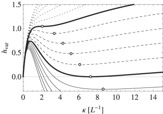
Figure 2: First order phase transition: The energy $h_{\rm var}$ versus the dimensionless inverse localization length $\kappa$, calculated for the trail wave function (3), for several values of the coupling constant $\alpha$. The dotted curves correspond to $\alpha<\alpha_{\rm min}^{\rm var}$, where the variational calculation predicts no polaron state. The upper thick curve corresponds to $\alpha=\alpha_{\rm min}^{\rm var}=350.0$. The dashed curves correspond to $\alpha_{\rm min}^{\rm var}<\alpha<\alpha_{c}^{\rm var}$ where the variational calculation predicts a meta-stable polaron state. The thick lower curve corresponds to $\alpha=\alpha_{c}^{\rm var}=431.5$. The solid curves correspond to $\alpha>\alpha_{c}^{\rm var}$ where the variational curve predicts a polaron ground state. Circles indicate the minima corresponding to the polaron state.

Note as an aside that, to leading order in $\kappa$, we find $h_{\rm eff}=8\kappa/3$, consistent with the discussion in the previous paragraph. Figure 2 shows $h_{\rm var}$ versus $\kappa$ for various values of $\alpha$.

The best estimate for the energy for given $\alpha$ is obtained by minimizing $h_{\rm var}(\kappa)$ with respect to $\kappa$ on the interval $[0,\infty)$. The following results are found: For $\alpha<350.0$ (dotted curves in Figure 2), $h_{\rm var}$ is a monotonically increasing function of $\kappa$ so that the minimum is $h_{\rm var}=0$ which occurs at $\kappa=0$. The implication is that here the ground state is extended. At $\alpha>\alpha^{\rm(var)}_{\rm min}=350.0$, a local minimum develops at $\kappa>\kappa_{\rm min}^{\rm var}=2.044$. For $\alpha^{\rm(var)}_{\rm min}<\alpha<\alpha^{\rm var}_{c}=431.5$ (dashed curves in Figure 2) this minimum has a positive energy and therefore corresponds to a meta-stable state. Finally, for $\alpha>\alpha^{\rm(var)}_{c}$ (thin solid curves in Figure 2), the energy of the polaron state becomes negative so that the polaron state is stable.

Next we numerically minimize $h[\phi,f]$ with respect to $\phi$ and $f$, with appropriate boundary conditions and subject to the constraint that $\phi$ is normalized. Details about the numerical method can be found in Appendix C.

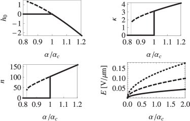
Figure 3: Results of the numerical calculation: In the top panels and in the bottom left panel, solid curves indicate ground state properties. Dashed curves indicate properties of the meta-stable polaron state. A thin vertical line indicates the value of $\alpha/\alpha_{c}$ below which no polaron solutions exist. The critical value of $\alpha$ is $\alpha_{c}=306.9$. Top left: The minimal values $h_{0}$ of the (dimensionless) energy $h[\phi,f]$ (cf. Eq. (2)) vs. $\alpha/\alpha_{c}$. Top right: The dimensionless inverse localization length $\kappa$ in the suspended part of the tube vs. $\alpha/\alpha_{c}$. Bottom left: The ratio $n=U/\hbar\omega_{0}$ between the bending energy and the lowest phonon energy vs. $\alpha/\alpha_{c}$. Bottom right: The electric field $E$ as a function of $\alpha/\alpha_{c}$, for a suspended section of length $L=1$ $\mu$m, and three different tube radii $r$. The solid curve is for $r=1$ nm, the dashed curve for $r=1.5$ nm and the dotted curve for $r=2$ nm.

Thus we find $\alpha_{c}=306.9$. (See the top-left panel of Figure 3.) This value of $\alpha_{c}$ is lower than the upper bound derived by means of the variational calculation above, as it should be. It is also of the same order of magnitude as the variational upper bound, indicating that the variational calculation is reasonably accurate. We further obtain the value of $\alpha_{\rm min}$, the smallest value of $\alpha$ for which polaron states exist as $\alpha_{\rm min}=254.5=0.8293\alpha_{c}$.

At $\alpha=\alpha_{c}$ we obtain a critical tip displacement $f_{c}(1)=0.138$. Reinstating units and eliminating the electric field in favour of $\alpha_{c}$ we obtain $y_{c}(L)/L=0.138\hbar\sqrt{\alpha_{c}/2m^{*}YIL}$. The critical tip displacement scales like $r^{-1}L^{1/2}$. For realistic values $L=1$ $\mu$m and $r=1$ nm, we find $y_{c}(L)=0.54$ nm.

We also calculate $n=U/\hbar\omega_{0}$, where $U$ is the bending energy and $\omega_{0}=3.52\sqrt{YI/\rho}/L^{2}$ r7 is the angular frequency of the lowest harmonic of the suspended tube. Here $\rho=0.671\,Mr/a_{0}^{2}$ is the mass per unit length of the tube, and $M$ is the mass of a carbon atom. Appendix D provides more detail. The quantity $n$, being the ratio between the energy stored in the deformed tube and the energy of a single phonon, is an estimate of the number of phonons involved in the tube deformation. In the lower left panel of Figure 3, $n$ is plotted as a function of $\alpha$. We see that when the transition to the polaron state occurs, there are on the order of a hundred phonons in the tube. The fact that $n$ is large in the polaron state provides additional a posteriori justification for treating the tube deformation classically.

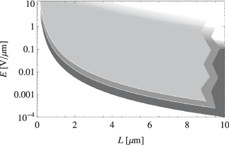
Figure 4: Phase diagram: The three different shaded regions correspond to different tube radii (assuming zig-zag tubes): The dark gray region is for $r=1$ nm, the gray region is for $r=1.5$ nm and the light gray region is for $r=2$ nm. In each case the shaded region indicates where the ground state is a polaron. At large $L$, the upper planes have been cut away to reveal the planes below. At large $E$ the shaded regions fade to white to emphasize that the upper boundaries of the shaded regions do not represent a phase transition.

An important question to ask is whether values of $\alpha$ that are of the order $\alpha_{c}$ and larger can be reached for realistic values of the length $L$, radius $r$, and external electric field $E$. Typical radii are of the order $1$ nm. Typical lengths are of the order $1$ $\mu$m. An upper bound on the electric field is provided by the breakdown field of the insulating elements in the setup. These are typically made of ${\rm SiO}_{2}$ for which the breakdown field is $\sim 10$ V/$\mu$m. In the bottom right panel of Figure 3, we plot the electric field $E$ versus the corresponding $\alpha$ for $L=1$ $\mu$m and three values of $r$ ranging from $1$ to $2$ nm. We see that producing a coupling constant in excess of $\alpha_{c}$ requires an electric field of $0.031$ V/$\mu$m for the thinnest tubes and $0.12$ V/$\mu$m for the thickest tubes. These are quite reasonable values, well below the breakdown field of ${\rm SiO}_{2}$. It is also of the same order as the field produced by an image charge in a metallic substrate $\sim 0.1$ $\mu$m below the cantelever.

It is informative to draw a phase diagram, indicating the region in parameter space where the ground state is of the polaron variety. There are two conditions that have to be met. Firstly, as we have discussed above, the coupling constant must be large enough, i.e. $\alpha(r,L,E)>\alpha_{c}=306.9$. There is however another condition: The deflection $y(L)$ of the tube’s free tip must be much smaller than the length $L$ of the suspended section. When $|y(l)|\simeq L$, the tube will likely come into contact with one of the surrounding elements of the setup, for instance the supporting substrate at $x=0$. Owing to van der Waals forces the tube will adhere to whatever it comes in contact with. When this happens, the coupling between electron motion and tube profile is destroyed. Of course, when this condition is not met, the small deflection approximation, on which our analysis relied, also breaks down. Appendix E provides more detail. In Figure 4 we show three cuts through the phase diagram in the $E$–$L$ plane, for $r=1,\,1.5,$ and $2$ nm respectively. In each case the polaron phase is indicated by a shaded region. We see that the value of the largest allowed electric field is always several orders of magnitude larger than the smallest allowed electric field.

In conclusion, we found that the coupling between the electron and the tube is controlled by a dimensionless coupling constant $\alpha=2m^{*}(eE)^{2}L^{5}/\hbar^{2}YI$. At strong coupling (large $\alpha$) the ground state of the system is a polaron, i.e. the electron is trapped in the deformation of the cantilever that it itself produces. As the coupling is decreased beyond the critical value of $\alpha_{c}=306.9$, a first order phase transition occurs. Below the transition point, the ground state consists of an undeformed tube and an extended electron wave function. For realistic values $L=1$ $\mu$m for the length of the suspended tube and $r=1$ nm for the tube radius, an electric field of $0.031$ V/$\mu$m is required to realize the polaron phase and the critical tip displacement is $0.54$ nm. The magnitude of the threshold electric field is the same as that produced by an image charge in a metallic substrate $0.10$ $\mu$m below the cantelever.

In future work we plan to study the nonlinear dynamics of a single polaron as well as the interaction between polarons in the same or adjacent suspended tubes. The eventual aim is to exploit the coupling between mechanical and electrical degrees of freedom for the coherent manipulation of the quantum state of the polaron.

Appendix A Expanding the energy in small $\kappa$

In the main text it is stated that at small inverse localization lengths $\kappa$, the energy $h$ is dominated by a positive contribution of order $\kappa$. Here we provide a detailed analysis.

Setting

$$\frac{\delta}{\delta\phi(x)}(h-\varepsilon\int_{-\infty}^{1}dz\,\phi^{2})=\frac{\delta}{\delta f(x)}(h-\varepsilon\int_{-\infty}^{1}dz\,\phi^{2})=0$$ (4)

and using the boundary conditions

$$\phi(z=1)=\lim_{z\to-\infty}\phi(z)=0,$$ (5a)

$$f(z=0)=\partial_{z}f(z=0)=0,$$ (5b)

$$\partial^{2}_{z}f(z=1)=\partial^{3}_{z}f(z=1)=0,$$ (5c)

we obtain two differential equations

$$\varepsilon\phi(z) = -\partial_{z}^{2}\phi(z)+\alpha f(z)\phi(z),$$ (6a)

$$\partial_{z}^{4}f(z) = -\phi(z)^{2}.$$ (6b)

Here $\varepsilon$ is a Lagrange multiplier that enforces the normalization of $\phi$. The first of these equations is the Schrödinger equation for the electron in a potential $\alpha f(z)$. The second equation describes the balance of the electrostatic force that deforms the tube and the elastic restoring force.

The solution to Eq. (6b) that satisfies the boundary conditions (5b) and (5c) is

$$f_{\phi}(z)=-\frac{1}{6} \left[\int_{0}^{z}dz^{\prime}\,(z^{\prime})^{2}(3z-z^{\prime})\phi(z^{\prime})^{2}\right.$$

$$+\left.\int_{z}^{1}dz^{\prime}\,z^{2}(3z^{\prime}-z)\phi(z^{\prime})^{2}\right].$$ (7)

We can substitute this solution into $h$ in order to obtain an effective energy functional that depends on $\phi$ only, i.e. $h_{\rm eff}[\phi]=h[\phi,f_{\phi}]$. By exploiting the fact that

$$\int_{0}^{1}dz^{\prime}\,(\partial_{z}^{2}f_{\phi})^{2}=\int_{0}^{1}dz^{\prime}\,f_{\phi}\partial_{z}^{4}f_{\phi}=-\int_{0}^{1}dz^{\prime}f_{\phi}\phi^{2},$$ (8)

we obtain

$$h_{\rm eff}[\phi]=\int_{-\infty}^{1}dz\,(\partial_{z}\phi)^{2}+\frac{\alpha}{2}\int_{0}^{1}dz\,f_{\phi}\phi^{2}.$$ (9)

We now expand $h_{\rm eff}$ in the inverse localization length $\kappa$ of the polaron state. Let us firstly look at the kinetic energy. We consider separately the contribution of the wave function in the supported and suspended parts of the tube. As mentioned before, the wave function is of the form $\phi=\phi_{0}e^{\kappa z}$ in the supported part of the nanotube. In the limit $\kappa\ll 1$, the normalization constant $\phi_{0}$ is of the order $\sqrt{\kappa}$. For the kinetic energy density integrated over the supported part of the tube, we obtain

$$\int_{-\infty}^{0}dz\,(\partial_{z}\phi)^{2}=\kappa^{2}\int_{-\infty}^{0}dz\,\phi^{2}\sim\kappa^{2}.$$ (10)

(In the last step we approximated $\int_{-\infty}^{0}dz\,\phi^{2}\simeq 1$, neglecting the possibility to find the electron in the region $0<z<1$, which is valid for $\kappa\ll 1$.) To estimate the kinetic energy stored in the suspended part of the tube, we note that here $\phi$ changes from $\phi_{0}\sim\sqrt{\kappa}$ at $z=0$ to $\phi=0$ at $z=1$. This corresponds to a typical slope $\partial_{z}\phi\sim-\sqrt{\kappa}$ so that

$$\int_{0}^{1}dz\,(\partial_{z}\phi)^{2}\sim\kappa$$ (11)

Thus, at small $\kappa$, the kinetic energy is dominated by a contribution of order $\kappa$. Note also that the kinetic energy is positive. To estimate the remaining term (=$\alpha\int_{0}^{1}dz\,f_{\phi}\phi^{2}$) in $h_{\rm eff}$ we note from that Eq. (7) that $f_{\phi}\phi^{2}$ is quartic in $\phi$. The integral therefore scales like $\phi_{0}^{4}\sim\kappa^{2}$. It is also negative.

Appendix B Variational calculation

In the main text we discuss a variational calculation in order to obtain an estimate $h_{\rm var}(\kappa)$ of the energy of the polaron state, that depends on a single variational parameter $\kappa$. In Fig. 2 of the main text, $h_{\rm var}(\kappa)$ is plotted for several values of the coupling constant $\alpha$. Here we give the explicit formula for $h_{\rm var}(\kappa)$. It is a rational function

$$h_{\rm var}(\kappa)=\frac{\sum_{n=0}^{6}(a_{n}-b_{n}\alpha)\kappa^{n}}{\sum_{n=0}^{6}c_{n}\kappa^{n}},$$ (12)

with coefficients

$n$	$a_{n}$	$b_{n}$	$c_{n}$
0	0	0	225
1	600	0	480
2	1165	1.639	466
3	990	2.151	254
4	445	1.087	81
5	105	0.2498	14
6	10	0.02205	1

Appendix C Numerical calculation

In the main text we present results of a numerical minimization of the energy $h$. Here we provide some details about the numerical method.

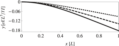
Figure 5: Numerically computed polaron states: Tube profiles $y(x)$ and wave functions $\psi(x)$ that solve Eqs. (6a) and (6b) for three different values of the coupling constant $\alpha$. The solid curves are for $\alpha=500=1.629\alpha_{c}$. Since $\alpha>\alpha_{c}$ for the solid curves, they represent the ground state of the system at this particular value of $\alpha$. The dashed curves are for $\alpha=306.9=1.00\alpha_{c}$. Since $\alpha=\alpha_{c}$ for these curves, they occur at the boundary between stability, where the energy of the polaron state is negative, and meta-stability where the energy of the polaron state is positive. The dotted curves are for $\alpha=254.5=0.8293\alpha_{c}=\alpha_{\rm min}$. There are no polaron states for $\alpha<\alpha_{\rm min}$.

We extremize the energy functional $h$ by solving solving Eqs. (6a) and (6b) numerically, subject to the boundary conditions (5a), (5b) and (5c). We use an iterative procedure. In each iteration we substitute a guess $f_{n}(z)$ for the tube profile into the Schrödinger equation (6a). The associated normalized ground state wave function $\phi_{n}(z)$ and electron ground state energy $\varepsilon_{n}$ is computed. The wave function $\phi_{n}$ is then substituted into Eq. (7). This is used as the next guess $f_{n+1}(x)$ for the tube profile, and the process is repeated until the change in electron energy $|\varepsilon_{n+1}-\varepsilon_{n}|$ is smaller than the required accuracy $\delta$. We choose $\delta=10^{-4}$, and an initial guess for the tube profile

$$f_{1}(z)=-\frac{1}{6}z^{2}(3-z).$$ (13)

This would have been the exact tube profile (cf. Eq. (7)), had the electron been localized right at the tip (z=1) of the tube. In each iteration the total energy is also calculated, and we check that it decreases in each iteration of the calculation. This gaurantees that the obtaind solution is a minimum.

We find that for $\alpha$ larger than about $1.1\alpha_{\rm min}$, convergence is obtained within less than $20$ iterations, while for smaller $\alpha$ up to $120$ iterations are required. In Figure 5 we show (converged) tube profiles and wave functions calculated with this procedure for three different values of $\alpha$.

The value of $\alpha_{\rm min}$, the smallest value of $\alpha$ for which polaron states exist, is obtained by repeating the iterative numerical calculation for smaller and smaller $\alpha$, until no amount of iteration produces convergence any more. We find that for smaller and smaller $\alpha$ down to $254.518$, the number of iterations required to obtain convergence slowly increases up to $120$. Then for $\alpha=254.510$, there is a sudden jump, and after $200$ iterations, convergence is still not obtained. We conclude that $\alpha_{\rm min}=254.51=0.8293\alpha_{c}$.

Appendix D The parameter dependence of the phonon-number $n$

In Fig. 3 of the main text the phonon-number $n$ is plotted as a function of the coupling constant $\alpha$. Here we show that indeed, $n$ does not depend on $L$ and $r$ separately, but only on $\alpha$, since this is not clear a priori. (The above statement holds subject to the approximation $I=\pi gr^{3}$, which is valid when $g\ll r$. A more sophisticated approximation for $I$ yields only a very weak $r$ dependence in the regime of realistic radii.)

Note firstly that $\omega_{0}$ is given by

$$\omega_{0}=\frac{3.52}{L^{2}}\sqrt{\frac{YI}{\rho}},$$ (14)

where $\rho$ is the mass per unit length of the tube, which is proportional to the tube radius. (The proportionality constant is $1.47\times 10^{4}\,m_{e}/a_{0}^{2}$.) Since $I$ is proportional to $r^{3}$, $\omega_{0}$ is proportional to $r/L^{2}$. The bending energy on the other hand can be written as

$$U_{0}=-\frac{\hbar^{2}}{4m^{*}L^{2}}\alpha\int_{0}^{1}dz\,f_{\phi}\phi^{2}.$$ (15)

Since the effective electron mass $m^{*}$ is proportional to $1/r$, $m^{*}L^{2}\omega_{0}$ is independent of $r$ and $L$ so that $n=U_{0}/\omega_{0}$ is a function of $\alpha$ only.

Appendix E Estimating when $|y(L)|\simeq L$

In the main text the phase diagram of the system is discussed. We limit our discussion of the polaron phase to the regime $|y(L)|<\simeq L$. This gives rise to the upper boundaries of the shaded regions in Fig. 4 of the main text. The estimate for $y(L)~{}L$ was obtained as follows: We firstly note that $|y(L)|<|y_{\rm max}|$ where $|y_{\rm max}|$ is the deflection produced when the electron is completely localized at $x=L$. From Eq. 13 we have $|y_{\rm max}|=eEL^{3}/3IY$. Thus, we demand that $1>eEL^{2}/3IY$.

- (1) V. A. Popov, Material Science and Engineering R 43, 61, (2004). K. L. Ekinci and M. L. Roukes, Rev. Sci. Instrum. 76, 061101, (2005).
- (2) G. A. Steele, A. K. Hüttel, B. Witkamp, M. Poot, H. B. Meerwaldt, L. P. Kouwenhoven, and H. S. J. van Zant, Science 325, 1103, (2009).
- (3) J. Gao, Q. Wang, and H. Dai, Nature Mater. 4, 745, (2005). G. A. Steele, G. Götz, and L. P. Kouwenhoven, Nature Nanotech. 4, 363, (2009).
- (4) M. R. Buitelaar, A. Bachtold, T. Nussbaumer, M. Iqbal, and C. Schönenberger, Phys. Rev. Lett. 88, 156801, (2002). P. Jarillo-Herrero, J. Kong, H. S. J. van der Zant, C. Dekker, L. P. Kouwenhoven, and S. De Franceschi, Phys. Rev. Lett. 94, 156802, (2005).
- (5) A. K. Hüttel, G. A. Steele, B. Witkamp, M. Poot, L. P. Kouwenhoven, and H. S. J. van Zant, Nano Lett. 9, 2547, (2009).
- (6) J. M. Kinaret, T. Nord, and S. Viefers, App. Phys. Lett. 82, 1287, (2003).
- (7) P. Poncharal, Z. L. Wang, D. Ugarte, and W. A. de Heer, Science 283, 1513, (1999).
- (8) L. D. Landau, Phys. Z. Sovietunion 3, 644, (1933). A. S. Alexandrov and N. F. Mott, Polarons and Bipolarons, (World Scientific, Singapore, 1995).
- (9) M. Verissimo-Alves, R. B. Capaz, B. Koiller, E. Artacho, and H. Chacham, Phys. Rev. Lett. 86, 3372, (2001). L. S. Brizhik, A. A. Eremko, B. M. A. G. Piette, and W. J. Zakrzewski, J. Phys. Condens. Mat. 19, 306205, (2007).
- (10) J. W. Ding, X. H. Yan, and J. X. Cao, Phys. Rev. B 66, 073401, (2002). O. Gülseren, T. Yildirim, and S. Ciraci, Phys. Rev. B 65, 153405, (2002).
- (11) L. D. Landau and E. M. Lifshitz, Theory of Elasticity, (Addison-Wesley, Massachusetts, 1959). M. Poot, B. Witkamp, M. A. Otte, and H. S. J. van Zant, Phys. Stat. Sol. (b), 244, 4252, (2007).
- (12) A. Krishnan, E. Dujardin, T. W. Ebbesen, P. N. Yianilos, and M. M. J. Treacy, Phys. Rev. B 58, 14013, (1998).