Voter Model with Time dependent Flip-rates

Abstract

We introduce time variation in the flip-rates of the Voter Model. This type of generalisation is relevant to models of ageing in language change, allowing the representation of changes in speakers’ learning rates over their lifetime. and may be applied to any other similar model in which interaction rates at the microscopic level change with time. The mean time taken to reach consensus varies in a nontrivial way with the rate of change of the flip-rates, varying between bounds given by the mean consensus times for for static homogeneous (the original Voter Model) and static heterogeneous flip-rates. By considering the mean time between interactions for each agent, we derive excellent estimates of the mean consensus times and exit probabilities for any time scale of flip-rate variation. The scaling of consensus times with population size on complex networks is correctly predicted, and is as would be expected for the ordinary voter model. Heterogeneity in the initial distribution of opinions has a strong effect, considerably reducing the mean time to consensus, while increasing the probability of survival of the opinion which initially occupies the most slowly changing agents. The mean times to reach consensus for different states are very different. An opinion originally held by the fastest changing agents has a smaller chance to succeed, and takes much longer to do so than an evenly distributed opinion.

Keywords: Stochastic processes, Population dynamics (Theory), Interacting agent models

1 Introduction

Neutral diffusion-like or copying process models have been applied in a very broad range of fields, from social phenomena [1] and language change [2, 3], to ecology [4, 5, 6] and population genetics [7] among many more. In all such models, different alternative items – species, opinions or language variants for example – are copied between neighbouring sites until one finally dominates the whole system. Here we consider the effect of time variation in the rate of update at each site in such models. This has particular relevance to language change, in which the rate at which speakers adapt to their language environment changes with age. The items copied are alternative variants of a language element; different ways of ‘saying the same thing’. Young speakers adapt very quickly, but once they reach adulthood many speakers barely change their language use [8, 9]. We show that the time to reach consensus depends in a non trivial way on the time scale of the variations of agent update rate, see fig. 1. By considering the mean time between interactions for each agent, we are able to obtain excellent estimates of the mean time to reach consensus, even in the intermediate regime where the timescale of consensus formation and the time scale of flip-rate change are of the same order, and interact in a non-trivial way.

The generalisation and the methods we will describe could be applied to any of the models mentioned, but for simplicity we concentrate on the Voter Model [10], in which agents in a population possess one of two discrete opinions. At each step an agent is chosen and imports the opinion of a randomly selected neighbour. The rate at which a particular agent is chosen for update is their flip-rate, and it is time variance of these flip-rates that we consider in this paper. The Voter Model has become an emblematic opinion spreading model due to its simplicity and tractability, as well as its distinction from other coarsening phenomena such as the Ising model [11]. The original Voter Model has been extended to include network structure [12, 13, 14] and the effect of changes in the microscopic interactions [15, 16]. Masuda et al. investigated the effect of heterogeneity in the flip-rates of agents [17]. While they have some spirit in common, the present model differs from other time dependent models including such effects as latency or ageing of states [18, 19, 20] in that the change in flip rate doesn’t depend on the opinion or the time of adoption of the opinion. That is, we are not interested in ageing of the opinions but of the agents themselves. The present work is probably most similar to the ‘exogenous update’ rule of [20], however in that case the update rule is the same for all agents and is reset when an agent becomes available for update, rather than changing independently .

In the heterogeneous Voter Model [17], a population of $N$ agents (labelled $i=1,2,...,N$) possess opinions $x_{i}$ which take values either $1$ or $0$. Agents are selected for update asynchronously with frequency proportional to flip-rates $r_{i}$, which may be different for each agent. Update consists of an agent importing the opinion of a neighbour, selected uniformly at random. In the present study, we extend this model to consider the flip-rates to be time dependent, thus $r_{i}(t)$. The method described here is perfectly amenable to considering complex network structure. For simplicity, we first consider a well mixed population (that is, a fully connected network) before examining more complex structures.

The mean time to consensus for homogeneous flip-rates $r_{i}=r,\;\forall i$, that is, the standard Voter Model, is well established [12, 21, 22], and is found by assuming the population of agents relaxes quickly to a quasi stationary state (QSS), followed by a much longer period characterised by collective motion. The mean time to consensus can be calculated for this second stage by writing a Fokker-Planck equation for a conserved centre-of-mass variable. This gives a lower bound and a good approximation to the total mean time to consensus. When heterogeneity is introduced in the flip-rates, the consensus time is always increased, and can be predicted from the moments of the flip-rate distribution [17]. For very slowly changing flip-rates, the consensus time is essentially the same as for the static heterogeneous case. For very quickly changing flip-rates, the consensus time may be reduced to the value found for homogeneous flip-rates with the same mean. For intermediate periods, the time to consensus varies smoothly between these two extremes, as can be seen in fig. 1. Using the distribution of flip-rates existing in the population simply returns the static heterogeneous result, which doesn’t vary with the period of variation of the flip-rates. Instead, we calculate effective flip-rates, found by considering the mean time between interactions for each agent. Using the moments of the distribution of these effective flip-rates returns the correct qualitative behaviour, and is in excellent quantitative agreement with numerical results (fig. 1).

2 Analysis

The mean time to consensus can be calculated through a Fokker-Planck Equation (FPE) formalism. See for example [21, 12] or the rigorous treatment in [22]. The essential idea is that after an initial, rapid, period of mixing, the individual opinions settle into a long lived meta-stable distribution. This quasi-stationary state (QSS) is characterised by a weighted mean opinion which is conserved by the dynamics. The mean time to consensus can be calculated by considering the evolution of only this central variable.

2.1 Mean consensus time for static flip-rates

For orientation, we first calculate the mean consensus times for static homogeneous (i.e. the basic Voter Model) and static heterogeneous flip-rates. We define a weighted mean opinion $\xi(t)$ by:

$$\xi(t)\equiv\frac{\sum_{i}{x_{i}(t)}/{r_{i}}}{\sum_{i}{1}/{r_{i}}}=\sum_{i}Q_{i}x_{i}(t)\;$$ (1)

where

$$Q_{i}\equiv\frac{1}{N\overline{({1}/{r})}}\;\frac{1}{r_{i}}$$ (2)

and $\overline{(\;\cdots\;)}$ signifies a population average. We choose $\xi$ because it is conserved by the dynamics [23, 24, 15, 21]:

$$\frac{{\rm d}}{{\rm d}t}\langle\xi(t)\rangle=0.$$ (3)

This also means that the probability that the population eventually reaches consensus in the state ${\bf 1}$ is simply

$$P({\bf x}\to{\bf 1})=\xi(0)\equiv\xi_{0}.$$ (4)

The fraction $x(t)\equiv\frac{1}{N}\sum_{i}x_{i}(t)$ of agents in the population holding opinion $1$, equivalently the ‘magnetisation’ converges rapidly to $\xi_{0}$:

$$\frac{{\rm d}\langle x\rangle}{{\rm d}t}=\langle x\rangle-\xi_{0}\,,$$ (5)

as do in turn the expected values of the individual opinions $x_{i}$:

$$\frac{{\rm d}\langle x_{i}\rangle}{{\rm d}t}=\frac{r_{i}(t)}{Nr_{0}}[\langle x_{i}\rangle-\langle x\rangle]\,.$$ (6)

After this initial mixing the system is in a long-lived quasi-stationary state (QSS) in which the individual opinions are subordinated to the centre-of-mass variable $\xi(t)$, which changes only very slowly. The QSS is found by setting $x=\xi$ and calculating the distribution of the $x_{i}$ about a fixed $\xi$. We can calculate the mean time, $T^{*}$, to reach consensus beginning from this QSS by considering only the central variable $\xi(t)$.

The conservation of $\langle\xi\rangle$ means that the FPE for the probability distribution of $\xi(t)$ has only a diffusion term, originating from the second jump moment:

$$\langle\delta\xi^{2}\rangle=\frac{1}{\bar{r}\overline{(\frac{1}{r})}N(N-1)}\left[\xi(1-x)+x(1-\xi)\right]\,.$$ (7)

Choosing the time increment $\delta t=1/N$, in the limit of large $N$ we arrive at

$$\frac{\partial}{\partial t}P(\xi,t^{\prime})=\frac{1}{\bar{r}\overline{(\frac{1}{r})}N}\frac{\partial^{2}}{\partial\xi^{2}}\left[\xi(1-\xi)P(\xi,t^{\prime})\right]\;,$$ (8)

where we have used the fact that in the QSS $x=\xi$. We use $t^{\prime}$ to emphasise that the QSS is now taken as the starting point. Thus $t^{\prime}=0$ when we first arrive in the QSS (at some time $t^{*}$, that is $t^{\prime}=t-t^{*}$).

Note that the state variables $x_{i}$ are discrete. It is however also possible to write a complete FPE in continuous variables, either by assuming a large population and aggregating all agents with $r_{i}$ in the range $[r_{i},r_{i}+\delta r)$ [12], or by considering each agent to be occupied by a number $M$ of particles. For $M\to\infty$, $x_{i}$ becomes a continuous variable. It was shown in [22] that if the rate of exchange of particles between agents is much slower than the copying within an agent, the results for large $M$ apply to the original case $M=1$.

The mean time taken to reach consensus then obeys the backward-FPE [25]

$$-1=\frac{1}{\bar{r}\overline{(\frac{1}{r})}N}\xi_{0}(1-\xi_{0})\frac{{\rm d}^{2}}{{\rm d}\xi_{0}}T^{*}\;.$$ (9)

Because $\xi$ is conserved, we use the initial value $\xi_{0}$ which is equal to the expected value of $\xi(t^{*})$ in the QSS. In the fully connected, and indeed in many other networks we might consider [21, 22], $t^{*}\ll T$, so we can use $T^{*}$ as a proxy for the overall mean time to consensus $T$. The mean flip-rate $r_{0}$ merely determines an overall time scale, so we can, without loss of generality, also set $r_{0}=1$. Furthermore, for large populations we can use the moments $\mu_{k}$ of $p(r)$ in place of population averages $\overline{r^{k}}$, so that $\overline{(1/r)}\to\mu_{-1}$. Solving eq. (9) then gives

$$T_{\mbox{het}}\approx N\mu_{-1}\left[\xi_{0}\ln\xi_{0}+(1-\xi_{0})\ln(1-\xi_{0})\right]\;.$$ (10)

This agrees with the result obtained previously in [17].

In the homogeneous flip-rate case, $\xi_{0}=x_{0}$, and $\mu_{-1}=1/\mu_{1}=1$, so that we recover the standard result

$$T_{\mbox{hom}}\approx N\left[x_{0}\ln x_{0}+(1-x_{0})\ln(1-x_{0})\right]\;.$$ (11)

2.2 Time-dependent flip-rates

Now we are ready to consider the case where the flip rates $r_{i}(t)$ can vary with time. We assume that the flip-rates $r_{i}(t)$ follow some periodic function with the period $S$ acting as a control variable. Initial values for $r_{i}$ are chosen by selecting $s_{i}$ uniformly at random from $[0,1)$ and setting $r_{i}(0)=f(s_{i})$ for some $f(s)$. It is convenient to ensure a stable distribution of $r_{i}$ values in the population over time. In the language change application, this corresponds to a stable distribution of speaker ages in a population, with old speakers periodically replaced by young ones, and whose members’ learning rates all follow the same function of age [i.e. $r(s)$]. This is obviously a very crude model, and our aim here is simply to demonstrate the general effect of time variation in such interactions. To achieve this, we define a periodic version of $f(s)$: let $r(s)\equiv f(s-\lfloor s\rfloor)$. For an agent with initial flip rate $r_{i}(0)=r(s_{i})$, we set

$$r_{i}(t)=r\left(s_{i}+\frac{t}{S}\right)\;.$$ (12)

This ensures the period is equal to $S$ and also that at any time, the overall distribution of $r_{i}(t)$ values in a large population follows $p[r(s)]{\rm d}r={\rm d}f(s)/{\rm d}s$.

We postulate that the change in observed consensus time is due to an interaction between the time scales of flip-rate change and of opinion change (or consensus formation) of the population. When the flip-rates change extremely slowly, consensus will be reached with essentially no change in flip-rates, hence the static heterogeneous result eq. (10) applies. If the flip-rates change extremely quickly, agent $i$ will cycle through all the possible values of $r_{i}$ in a very short time compared with the rate at which she interacts. We can therefore calculate an approximate consensus time by replacing $r_{i}$ with $\langle r_{i}\rangle_{t}=r_{0}$. We see, then, that in the limit of very quickly changing flip-rates $T$ is given by eq. (11) i.e. the consensus time in the standard homogeneous Voter Model. The heterogeneous flip-rate consensus time (10) and the fast change limit (11) provide approximate upper and lower bounds for the consensus time. As can be seen in fig. 1, these bounds agree very well with numerical results in the two limits, and consensus times for intermediate regimes lie between the two.

We can calculate a more rigorous interpolation between the results (10) and (11) by observing that in both cases, the weight for each agent’s state in the sum for $\xi(t)$ in eq. (1) is proportional to $1/r_{i}$, which is the expected time interval between interactions for agent $i$. For intermediate $S$, let us generalise by defining $\tau_{i}(t)$ to be the expected interval between interactions for agent $i$, where the dependence on $t$ indicates that this update interval varies because $r_{i}(t)$ varies with time. Consider a sequence of short intervals of length $\Delta t$, beginning at time $t$. The probability that $i$ is selected in the first interval is $r_{i}(t)\Delta t$. The probability that $i$ is selected in the second (having not been selected in the first) is $[1-r_{i}(t)\Delta t]r_{i}(t+\Delta t)\Delta t$, and so on. The probability that $i$ is selected in the $(k+1)$-th such interval is thus:

$$r_{i}(t+k\Delta t)\Delta t\prod_{l=0}^{k-1}[1-r_{i}(t+l\Delta t)\Delta t]\;.$$ (13)

Taking $\Delta t\to 0$ we can write the terms in the product as exponentials, i.e. $1-r_{i}(t+l\Delta t)\Delta t\to\exp\{-r_{i}(t^{\prime\prime}){\rm d}t\}$, where we have rewritten $t+k\Delta t\to t^{\prime}$ and $t+l\Delta t\to t^{\prime\prime}$. The product then becomes an integral in the argument of the exponential, so that the probability that $i$ is selected in the interval $[t^{\prime},t^{\prime}+{\rm d}t)$ becomes

$$r_{i}(t^{\prime}){\rm d}t\exp\left\{-\int_{t}^{t^{\prime}}r_{i}(t^{\prime\prime}){\rm d}t^{\prime\prime}\right\}\;.$$ (14)

Multiplying by the waiting times $(t^{\prime}-t)$ and integrating gives the expected waiting time

$$\tau_{i}(t)=\int_{t}^{\infty}(t^{\prime}-t)r_{i}(t^{\prime})\exp\left\{-\int_{t}^{t^{\prime}}r_{i}(t^{\prime\prime}){\rm d}t^{\prime\prime}\right\}{\rm d}t^{\prime}\,.$$ (15)

We can then define an effective flip-rate

$$\tilde{r}_{i}(t)\equiv\frac{1}{\tau_{i}(t)}.$$ (16)

For the static case, we recover $\tilde{r}_{i}(t)=r_{i}$. For extremely quickly varying $r_{i}(t)$, $\tilde{r}_{i}(t)=\bar{r}$, which is the same value as obtained in the original homogeneous Voter Model. To see this, notice that fluctuations in $\int_{t}^{t^{\prime}}r(t^{\prime\prime}){\rm d}t^{\prime\prime}$ die out very quickly, so after some small time $\sigma$, $\exp\{-\int_{t}^{t^{\prime}}r_{i}(t^{\prime\prime}){\rm d}t^{\prime\prime}\}\approx\exp\{-(t^{\prime}-t){\bar{r}}\}$, while for times less than $\sigma$, the exponential term is close to $1$ and $\int_{t}^{t+\sigma}(t^{\prime}-t)r_{i}(t^{\prime}){\rm d}t^{\prime}\approx\sigma^{2}{\bar{r}}$, giving $\tau_{i}(t)\approx\sigma^{2}r_{o}+e^{-\sigma{\bar{r}}}(1+\sigma{\bar{r}})/{\bar{r}}\approx 1/{\bar{r}}$. These limits agree with the two limits obtained through the qualitative arguments above.

For the reduction to a single variable, we then define

$$\tilde{\xi}(t)\equiv\frac{\sum_{i}\tau_{i}(t)x_{i}(t)}{\sum_{i}\tau_{i}(t)}\;.$$ (17)

The argument proceeds as before, so that we in effect replace $\overline{(1/r)}$ by $\overline{\tau_{i}(0)}$ and $\bar{r}$ by $\tilde{r}_{0}\equiv\overline{\tilde{r}_{i}(0)}$ in eq. (9), to give

$$-1=\frac{1}{N\overline{\tau_{i}(0)}\tilde{r}_{0}}\tilde{\xi}_{0}(1-\tilde{\xi}_{0})\frac{{\rm d}^{2}}{{\rm d}\tilde{\xi}_{0}}T^{*}\;.$$ (18)

For homogeneous initial conditions, $\tilde{\xi}_{0}=x_{0}$. We can utilise the fact that all agents follow the same flip-rate function $r(s)$, but starting at different initial values of $s$ to estimate $\overline{\tau_{i}(0)}$. In the large-$N$ limit, the agent’s initial values of $s_{i}$ evenly populate the interval $[0,1)$. For large $N$, then, we can replace the average over agents by an average over $s$, giving

$$\overline{\tau_{i}(0)}\approx\int_{0}^{1}\tau(s){\rm d}s\equiv\tau_{0}\;,$$ (19)

where $\tau(s)\equiv\tau_{i}(0)$ for $i$ such that $r_{i}(0)=r(s)$. Finally then we can write

$$T\approx N\tau_{0}\left[x_{0}\ln x_{0}+(1-x_{0})\ln(1-x_{0})\right]$$ (20)

for homogeneous initial conditions. This analytic calculation is in excellent agreement with numerical results for various $r(s)$ distributions over the whole range of $S$, as can be seen in fig. 1.

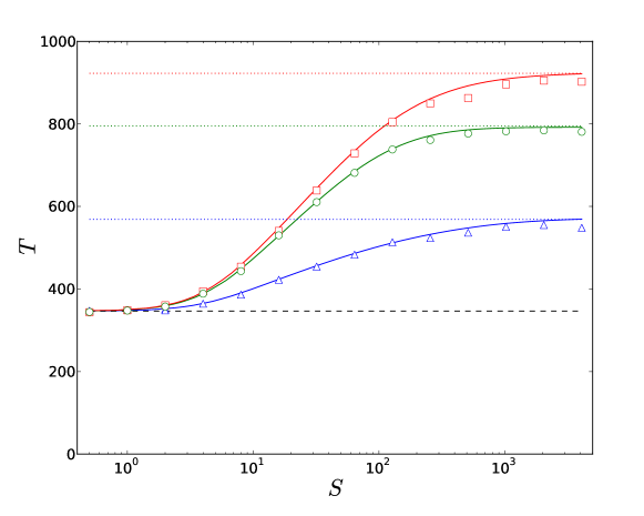
Figure 1: Mean consensus time $T$ as a function of period $S$ of change of flip-rates for three different flip rate functions $r(t/S)$. Numerical simulations are shown as open symbols for sinusoidal function $r_{\mbox{sin}}$ (circles), linear ‘sawtooth’ $r_{\mbox{lin}}$ (triangles) and quadratic sawtooth $r_{\mbox{qdr}}$ (squares). Solid curves are analytic calculations using eq. (20). Dashed line is mean consensus time $T_{\mbox{hom}}$ for homogeneous flip-rates, dotted lines for heterogeneous but static flip-rates, $T_{\mbox{het}}$. Simulation results are averages over $10^{4}$ runs with homogeneous initial conditions and population size $N=500$.

Higher moments can be calculated iteratively using equations [25]

$$-nT_{n-1}=\frac{1}{N\tau_{0}}\tilde{\xi}_{0}(1-\tilde{\xi}_{0})\frac{{\rm d}^{2}}{{\rm d}\tilde{\xi}_{0}}T_{n}\;,$$ (21)

where $T_{n}$ is the $n$^th moment of the consensus time distribution leading to expressions in terms of polylogarithm functions. The variance of consensus times calculated in this way is in excellent agreement with numerical simulations (not shown). In fact eq. (21) only differs from the ordinary voter model by a factor $\tau_{0}$, so the whole distribution of consensus times has the same shape as that for the ordinary voter model, once time is rescaled by $\tau_{0}$. This is borne out in simulations, see fig. 2.

2.3 Network Structure

In [15] it was shown that a similar mean-field approach is sufficient to reproduce the population size scaling of the mean consensus time on heterogeneous networks for the ordinary voter model. By assuming flip-rates to be independent of degree, a similar treatment can be performed here. We now show that the population size scaling for time varying flip-rates (and hence also for the heterogeneous flip-rate model of ref. [17]) depends on the network degree distribution in the same way as in the ordinary voter model.

We define the weighted mean to be

$$\xi(t)\equiv\frac{\sum_{i}{x_{i}(t)q_{i}}/{r_{i}}}{\sum_{i}{q_{i}}/{r_{i}}}$$ (22)

where $q_{i}$ is the degree of voter $i$. Because the probability that voter $i$ is chosen for update is proportional to $1/q_{i}$, we again find that $\xi$ is conserved by the dynamics. Carrying out averages over $q_{i}$ and $r_{i}$ separately (they are chosen independently), and, as before, replacing population averages with distribution moments we find, for large populations,

$$\langle\delta\xi^{2}\rangle\approx\frac{1}{r_{0}\mu_{-1}\langle q\rangle^{2}N^{3}}\sum_{q}n_{q}q^{2}\left[x(1-x_{q})+x_{q}(1-x)\right]\,.$$ (23)

Where $n_{q}$ is the number of voters having degree $q$, and $q$ is the mean opinion of such voters. Finally, in the QSS we set $x_{q}=x=\xi$ giving

$$\langle\delta\xi^{2}\rangle\approx\frac{\langle q^{2}\rangle}{r_{0}\mu_{-1}\langle q\rangle^{2}N^{2}}\xi(1-\xi)\,.$$ (24)

This differs from the fully connected result only by a factor $\langle q^{2}\rangle/\langle q\rangle^{2}$, and hence the mean consensus time for heterogeneous flip-rates on a network goes as

$$T\propto N\mu_{-1}\frac{\langle q\rangle^{2}}{\langle q^{2}\rangle}\;.$$ (25)

It follows that for time varying flip-rates and homogeneous initial conditions, the mean consensus time goes as [compare Eq. (20)]:

$$T\propto N\tau_{0}\mu_{-1}\frac{\langle q\rangle^{2}}{\langle q^{2}\rangle}\;.$$ (26)

As can be seen in fig. 6, this agrees with numerical simulation for Erdos-Renyi networks and for scalefree networks.

2.4 Inhomogeneous Initial Conditions

We now consider the effect of heterogeneity in the initial opinions of agents. For the static heterogeneous case, the probability $P({\bf x}\to{\bf 1})$ to reach consensus state ${\bf 1}$ also depends on the flip-rates of the agents. The opinion $1$ is more likely to achieve consensus if it initially occupies the more slowly changing agents, and vice-versa.

Returning to eq. (17), $\langle\tilde{\xi}\rangle$ is a conserved quantity to the extent that the replacement of $r_{i}(t)$ by $\tilde{r}_{i}(t)$ in the Fokker-Planck Equation (8) is a valid approximation. The probability to reach consensus in the state ${\bf 1}$ is then simply $\tilde{\xi}_{0}$. This probability varies with the period of change $S$ of the flip-rates. When the flip-rates change very fast, the agents are essentially identical (having effective flip rate $\bar{r}$) and so there is no initial configuration dependence. Conversely, the effect of initial inhomogeneity in opinion (that is, correlation between initial flip-rate and initial opinion) will be strongest for extremely slowly varying flip-rates. This can be seen in fig. 3.

The mean consensus time again obeys eq. (18), but the presence of inhomogeneous initial conditions is felt through the fact that now $\tilde{\xi}_{0}\neq x_{0}$, leading to

$$T\approx N\tau_{0}\left[\tilde{\xi}_{0}\ln\tilde{\xi}_{0}+(1-\tilde{\xi}_{0})\ln(1-\tilde{\xi}_{0})\right]\;.$$ (27)

This means we must calculate $\tilde{\xi}_{0}$ using the initial distribution of $x_{i}$. In the examples shown here this was done by integrating eq. (15) numerically and then computing eq. (17) as an integral over $s$ [compare eq. (19)] to find $\tilde{\xi}_{0}$. The value of $\tau_{0}$ depends only in $r(s)$ and $S$, so is independent of initial conditions. As for the homogeneous case, $\tau_{0}$ increases with $S$, and because the fastest change in $\tau_{0}(S)$ and $\tilde{\xi}_{0}(S)$ occur in different ranges of $S$ (compare fig. 1 with fig. 3) the final curve for $T(S)$ has the complicated shape seen in fig. 4, borne out in simulation.

To calculate the mean time to consensus at a particular state, we again solve eq. (18) but the appropriate boundary conditions are different. This gives

$$T_{0} \approx N\tau_{0}\frac{\tilde{\xi}_{0}}{(1-\tilde{\xi}_{0})}\ln\tilde{\xi}_{0}\;,$$ (28)

$$T_{1} \approx N\tau_{0}\frac{(1-\tilde{\xi}_{0})}{\tilde{\xi}_{0}}\ln(1-\tilde{\xi}_{0})\;.$$ (29)

Combining these two times in proportion to the probability to reach each state returns eq. (27).

3 Numerical Simulations

We performed simulations of the model with different distributions of $r_{i}$. We considered the following functional forms for $r(s)$, chosen to give some variety of interesting functional forms:

$$r_{\mbox{qdr}}(s) =r_{0}-r_{d}+3r_{d}(1-s+\lfloor s\rfloor)^{2},$$ (30)

$$r_{\mbox{sin}}(s) =r_{0}+r_{d}\sin(2\pi s),$$ (31)

$$r_{\mbox{lin}}(s) =r_{0}-r_{d}+2r_{d}(s-\lfloor s\rfloor).$$ (32)

The mean of each function is $\mu_{1}=r_{0}$, which we generally choose to be equal to $1$. The parameter $r_{d}$ controls the amplitude of the variations. To ensure the values of $r_{i}$ are always strictly positive, we require $r_{d}<r_{0}$. The mean time to consensus and probability to reach a certain final state depend only on the distribution of $r_{i}$ values in the population and on the period $S$. Careful consideration of eqs. (15) and (19) which involve integration over every possible interval of $r(s)$ leads to the conclusion that a reordering of the function $r(s)$ would lead to the same mean consensus time. For example, time reversed versions of any of the $r(s)$ functions would yield the same results.

The mean time to consensus for different flip-rate periods $S$ is presented in fig. 1 for the three $r(s)$ functions tried. All move from a time similar to that found for homogeneous $r_{i}$ (the original Voter Model) for small $S$ to a value close to that found for static $r_{i}$ with the same distribution (heterogeneous Voter Model) for large $S$. See eqs. (10) and (11) in Section 2. The transition occurs over a similar range of $S$ for each model, though the shape differs a little.

The distribution of consensus times rises rapidly to a peak value at small times, followed by a long tail very closely approximated by an exponential decay. In eq. (20) we see that the mean consensus times for different $r$ functions or values of $S$ differ only by the factor $\tau_{0}$. In fact, the whole distribution of consensus times has the same shape, so that if we rescale by $\tau_{0}$, the distributions collapse onto the same curve, as shown in fig. 2. In the inset the data are plotted against a logarithmic scale, showing the exponential tail clearly. Interestingly the decay $p_{T}\propto e^{-\lambda t}$ generally does not have $\lambda=1/T$ as might be naively expected.

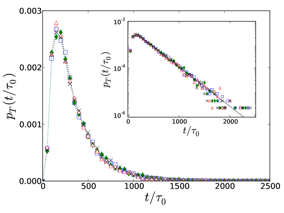
Figure 2: Distribution $p_{T}(t/\tau_{0})$ of consensus times rescaled by $\tau_{0}$ for $r_{\mbox{qdr}}(s)$ and $S=0.5$ ($\square$), $S=32$ ($\diamond$) and $S=2048$ ($\triangle$), and for $r_{\mbox{lin}}(s)$ with $S=128$ ($\times$). Frequencies were binned in rescaled time intervals of $50$. Under this time rescaling, all distributions collapse onto the same curve. Inset: the same data plotted with logarithmic vertical axis, compared with a decaying exponential function (line).

We also carried out simulations with inhomogeneous initial conditions. Because we have so far dealt only with a simple fully-connected (or well mixed) population, the inhomogeneity is in the correlation between initial $r_{i}$ values and initial opinions. Shown in figs. 3 and 4 are results for $r_{\mbox{sin}}(s)$. The agents were divided into two equal groups. Agents in the first group had $x_{i}(0)$ set to $0$, and $s_{i}(0)$ chosen uniformly in $[0,1/2)$. The agents in the second group had $x_{i}(0)$ set to $1$, and $s_{i}(0)$ chosen uniformly in$[1/2,1)$. In this way $x_{0}=1/2$ but the agents with initial opinion $1$ all had initial values of $r_{i}$ below $r_{0}$, while those with initial opinion $0$ all had $r_{i}(0)>r_{0}$. This means the probability to reach final state ${\bf 1}$ is greater than $x_{0}$. As can be seen in fig. 3, the effect is largest for large $S$.

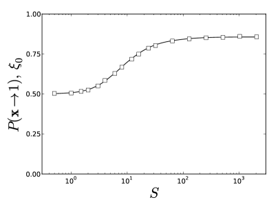
Figure 3: Probability to reach consensus at the state ${\bf 1}$ as a function of $S$ for inhomogeneous initial conditions. Open squares are simulation results for $r_{\mbox{sin}}(s)$. Half the agents have $x_{i}(0)=1$ and initial flip rate $r_{\mbox{sin}}(s_{i})$ with $s_{i}\in[1/2,1)$. Remaining agents have $x_{i}(0)=0$ and $s_{i}\in[0,1/2)$. Data points are from $2\times 10^{4}$ runs with $N=500$. Solid curve is $\tilde{\xi}_{0}$ calculated using eqs. (15) - (17).

As $S$ decreases, the timescale of change of $r_{i}$ eventually becomes shorter than the timescale of consensus, and the effect of the initial inhomogeneity is lost. The time to reach consensus also changes with $S$, as for the homogeneous case, but now in a more complicated way, fig. 4 (a). The inhomogeneity reduces the overall time to reach consensus from that found in the heterogeneous case, as can be seen by comparing the dotted and central solid curves in fig. 4 (b) , due to the inertia of the slowly changing agents, who now initially share a common opinion, combined with the speed with which the agents holding the weaker opinion may be changed.

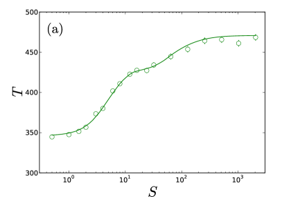
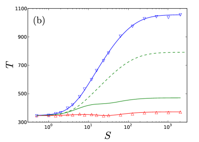
Figure 4: (a) Mean consensus time as a function of $S$ for inhomogeneous initial conditions. Open circles are simulation results for $r_{\mbox{sin}}(s)$. Solid curve is calculated consensus time using eq. (27). (b) Mean time to reach each of the two possible consensus states. ($\triangle$) mean time to reach final state ${\bf 1}$. ($\bigtriangledown$) mean time to reach final state ${\bf 0}$. Analytical predictions of eqs. (28) and (29) are shown as solid lines (blue and red respectively, online). For comparison the analytic predictions for the overall mean time to consensus (solid, green online) from eq. (27)—the same as shown in panel (a)—and for the homogeneous case (dashed) from eq. (20) are also shown. Simulation conditions are the same as for fig. 3.

It is also interesting to compare the mean time taken to reach each of the final states, ${\bf 0}$ and ${\bf 1}$. The mean time to reach ${\bf 1}$ is almost as short as (but not shorter than) that for homogeneous $r$. The agents originally holding opinion $1$ have a lot of weight, so the majority of agents in the mixed QSS will have opinion $1$ and quickly kill off opinion $0$. In the minority of cases, (see fig. 3) the final state is ${\bf 0}$. In this case, the time taken to reach consensus is very long, significantly longer then the time taken for heterogeneous $r$ with homogeneous initial conditions, as can be seen in fig. 4 (b). This has ramifications for language change, as age related variation in flip-rates delays consensus in two ways. The mean time to reach consensus, which corresponds to a language variant becoming established as the convention in a population, is always longer for heterogeneous flip-rates than for a perfectly homogeneous population, so any changes of learning with age will delay the establishment of a convention. The effect is exacerbated by the fact that new variants tend to originate in the youngest members of the population [26], corresponding to opinion $0$ in the present model, meaning the time taken for a new variant to overtake the population is even longer. For example, in [3] the mean time to reach consensus among British and Irish immigrants to New Zealand in a feasible neutral model was found to be much longer than the observed time. As just described, generational effects only make this situation worse, suggesting that some kind of selection effect (preference for one variant over another) must have been at work in this situation.

To establish the effect of system size, we repeated numerical simulations for a range of values of $N$, from $50$ up to $1000$. In fig. 5 (a) we plot $T$ as a function of $N$ for several values of $S$ across a broad range. We see that the mean consensus times grow linearly with $N$, confirming that the calculated scaling $T\propto N$ is correct. Numerical results are in excellent agreement with analytic predictions for larger $N$, given by by eq. (20). In fig. 5 (b) we plot the absolute difference between the numerical and analytic results as a function of $N$, for several $S$ values. We see that the results for small $N$ do not agree at all well with analytic predictions, which are based on a large $N$ approximation. For larger $N$, however, the numerical results quickly converge to the analytic curve, coinciding for $N\geq 400$. For small $S$, the difference is consistent with zero for $N$ from approximately $N=400$. For larger $S$ values, the numerical results never exactly converge to the prediction, but the difference achieves its minimum value from $N$ around $400$ and remains the same as $N$ increases (aside from statistical fluctuations). All of the results presented above are for $N=500$. Above this value we don’t expect to see any improvement in the results.

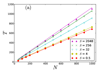
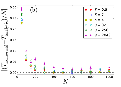
Figure 5: (a) Mean consensus time versus population size for different values of $S$, using $r_{\mbox{lin}}(s)$. Symbols show numerical results, lines show predictions of eq. (20) which grow linearly with $N$. (b) The difference between numerical and analytic values for $T/N$ as a function of $N$ at several values of $S$. For small $S$, the difference is large for small $N$ but converges rapidly to $0$. For larger $S$ the difference also falls rapidly, but converges to a small yet non zero value.

Finally, we extended the simulations to a population of voters on a network. We carried out simulations of the model for Erdős-Rényi networks and scalefree networks, whose degree distributions follow a decaying powerlaw of the form $P(q)\propto q^{-\gamma}$ for large degree $q$. The qualitative behaviour is exactly the same, with mean consensus time rising with a logistic-shaped curve from a minimum at small $S$ to a maximum at large $S$. Equation  (26) predicts that consensus times should depend on the degree distribution of an uncorrelated network by a factor $\langle q\rangle^{2}/\langle q^{2}\rangle$. In general, this factor does not depend on network size, meaning consensus times will grow linearly with $N$. If $\langle q^{2}\rangle$ diverges with $N$, a different scaling of mean consensus time with $N$ will emerge. For scalefree networks with $\gamma<3$, $\langle q^{2}\rangle\propto N^{(3-\gamma)/(\gamma-1)}$ meaning we expect to find $T\propto N^{(2\gamma-4)/(\gamma-1)}$. In fig. 6 we plot mean consensus time for various $N$ for an Erdős-Rényi network with mean degree $7$, and scalefree networks with $\gamma=3.5$ and $\gamma=2.5$. As expected, $T$ grows linearly with $N$ for the Erdős-Rényi network and scalefree network with $\gamma=3.5$. For $\gamma=2.5$ the mean consensus time grows sublinearly with $N$, with an exponent close to the expected value of $2/3$.

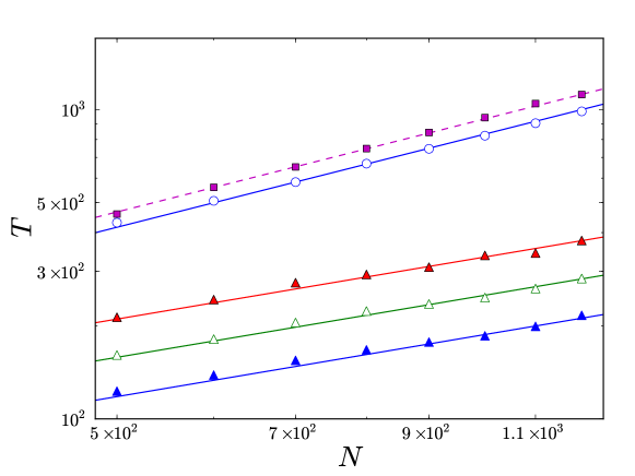
Figure 6: Mean consensus time $T$ versus population size $N$ on different networks, plotted on logarithmic axes. From top to bottom: Erdos-Renyi graph with mean degree $7$ ($\square$), scalefree graph with exponent $\gamma=3.5$ ($\circ$) and scalefree graph with $\gamma=2.5$ for $S=2048,32$ and $0.5$ (triangles). Solid lines are analytic predictions based on eq. (26) which predicts $T\propto N$ for Erdős-Rényi and scalefree with $\gamma=3.5$ and $T\propto N^{2/3}$ for $\gamma=2.5$. All data are for $r_{\mbox{lin}}(s)$ with $x_{0}=0.5$ and homogeneous initial conditions.

4 Discussion

In this paper we have introduced a generalisation of the Voter Model in which the flip-rates of agents vary with time. Interaction between the time scale of consensus formation and the time scale of flip-rate change leads to non-trivial dependence of mean consensus time on the period of flip-rate change. For very rapidly changing flip-rates, the mean time to consensus agrees with that found for the Voter Model with fixed homogeneous flip-rates. As the period of change of the flip-rates lengthens, so does the consensus time, until it saturates at the time found for static heterogeneous flip rates. An analytic estimate of the mean consensus time can be found by calculating the expected interval between interactions for each agent, then using the usual method of assuming a quickly reached quasi-stationary state followed by a slow escape to consensus. The mean consensus time is calculated for this second stage through a Fokker-Planck equation for a single conserved centre-of-mass variable. The results obtained by this method are in excellent agreement with numerical simulation. The overall mean time to consensus, the mean time to reach a particular final state and the rescaling of the distribution of consensus times are all correctly predicted. We also found that the complex network structures such as scale-free networks affect the scaling of the mean consensus time with population size in the same way that they do for static flip-rates.

For simplicity here we used periodic flip-rates, but the method used is readily applicable to more complex variations in flip-rates. For example, if each agent’s flip-rate varies with a different period, or indeed if each followed a different function entirely. More generally, time dependent interactions in any copying process may be modelled and analysed in a similar way, to consider for example seasonal variation in invasion rates in ecological models, or time-variation in the strength of synaptic interactions in neuronal models. This is particularly relevant to language change. Speakers learn more quickly when they are young and more slowly or almost not at all once they reach adulthood. The effect of such ageing can be modelled by exactly the kind of time-varying interactions described here. The results presented here for this very simple model suggest that in a more realistic language change model, heterogeneity in learning rates will increase the mean time taken to reach consensus, and this will be further exacerbated as a new language variant is more likely to appear in the faster learning (i.e. the younger) members of the population. The inertia of the (older) slowly adapting speakers will contribute both to enhanced survival probability for the existing convention, and in the event that a new variant does take over to increasing the time required for this to happen. Extension of time variation of update rates to such more realistic models is therefore a natural avenue for future investigation. Another possible extension would be to consider flip-rates that depend on local dynamical processes, which is relevant for example in the case of neuronal models in which a neuron’s response depends on recent activity.

References

- [1] Castellano C, Fortunato S and Loreto V 2009 Rev. Mod. Phys. 81 591–646
- [2] Baxter G J, Blythe R A, Croft W and McKane A J 2006 Phys. Rev. E. 73 046118
- [3] Baxter G J, Blythe R A, Croft W and McKane A J 2009 Language Variation and Change 21 257–296
- [4] Horvat S, Derzsi A, Neda Z and Balog A 2010 J. Theor. Biol. 265 517–523
- [5] Hubbell S 2001 The Unified Neutral Theory of Biodiversity (Princeton)
- [6] Condit R et al. 2002 Science 295 666–669
- [7] Crow J F and Kimura M 1970 An Introduction to Population Genetics Theory (New York: Harper and Row)
- [8] Bailey G, Wikle T, Tillery J and Sand L 1991 Language Variation and Change 3 241–264
- [9] Sankoff G 2005 Cross sectional and longitudinal studies Sociolinguistics: an International Handbook of the Science of Language and Society vol 2 ed Ammon U, Dittmar N, Mattheier K J and Trudgill P (Walter de Gruyter) pp 1003–1012 2nd ed
- [10] Liggett T M 1999 Stochastic Interacting Systems: Contact, Voter and Exclusion Processes (Berlin: Springer)
- [11] Dornic I, Chaté H, Chave J and Hinrichsen H 2001 Phys. Rev. Lett. 87 045701
- [12] Sood V and Redner S 2005 Phys. Rev. Lett. 94 178701
- [13] Suchecki K, Eguiluz V and San Miguel M 2005 Phys. Rev. E 72 036132
- [14] Baronchelli A, Castellano C and Pastor-Satorras R 2011 Phys. Rev. E 83 066117
- [15] Sood V, Antal T and Redner S 2008 Phys. Rev. E 77 041121
- [16] Schneider-Mizell C M and Sander L M 2009 J. Stat. Phys. 136 59–71
- [17] Masuda N, Gibert N and Redner S 2010 Phys. Rev. E 82 010103(R)
- [18] Stark H U, Tessone C J and Schweitzer F 2008 Phys. Rev. Lett. 101 018701
- [19] Lambiotte R, Saramaki J and Blondel V D 2009 Phys. Rev. E 79 046107
- [20] Fernández-Gracia J, Eguíluz V M and Miguel M S 2011 Update rules and interevent time distributions: Slow ordering vs. no ordering in the voter model arXiv:1102.3118 (Preprint arXiv:1102.3118)
- [21] Baxter G J, Blythe R A and McKane A J 2008 Phys. Rev. Lett. 101 258701
- [22] Blythe R A 2010 J. Phys. A: Math. Theor. 43 385003
- [23] Castellano C 2005 AIP Conf. Proc. 779 114–120
- [24] Suchecki K, Eguiluz V M and San Miguel M 2005 Europhys. Lett. 69 228
- [25] Gardiner C W 2004 Handbook of Stochastic Methods 3rd ed (Berlin: Springer)
- [26] Labov W 2001 Principles of linguistic change, Vol 2: Social factors (Oxford: Basil Blackwell)