Agent-based Versus Macroscopic Modeling of Competition and Business Processes in Economics

Abstract

Simulation serves as a third way of doing science, in contrast to both induction and deduction. The web based modeling may considerably facilitate the execution of simulations by other people. We present examples of agent-based and stochastic models of competition and business processes in economics. We start from as simple as possible models, which have microscopic, agent-based, versions and macroscopic treatment in behavior. Microscopic and macroscopic versions of herding model proposed by Kirman and Bass diffusion of new products are considered in this contribution as two basic ideas.

I Introduction

Statistically reasonable models of social systems, first of all stochastic and agent based, are of great interest for wide community of interdisciplinary researchers dealing with diversity of complex systems [1]. Computer modeling serves as a technique in the for finding relation between micro level interactions of agents and macro dynamics of the whole system. Nevertheless, some general theories or methods that are well developed in the natural and physical sciences can be helpful in the development of consistent micro and macro modeling of complex systems [1]. Our own modeling of financial markets by the nonlinear stochastic differential equations is based on the empirical analysis of financial data and power law statistics of proposed equations [2]. Reasoning of proposed equations by the microscopic interactions of traders (agents) looks as a tough task for such complex system. Apparently the development of macroscopic descriptions for the well established agent based models would be more consistent approach in the analysis of micro and macro correspondence. For such analysis one should select simple enough agent based models with established or expected corresponding macroscopic description. In this contribution we discuss few examples of agent based modeling in business and finance with corresponding macroscopic description of selected systems.

Kirman’s ant colony model [3] is agent-based model, which explains the importance of herding and individuality inside the ant colonies. As human crowd behavior is ideologically very similar, this model can be applied to and actually was built as framework for financial market modeling [3, 4, 5]. On our website, [6], we have presented interactive realizations of the original Kirman’s agent-based model (see [7]) and of it’s stochastic treatment by Alfarano et al. [4] (see [8]). Further we follow the works by Alfarano et al. [4, 5] and introduce our own model modifications in order to obtain more sufficient agent-based models of financial markets, which would have an alternative macroscopic description in the terms of Stochastic Calculus.

Diffusion of new products is a key problem in marketing research. Bass Diffusion model is a prominent model in diffusion theory introducing a differential equation for the number of adopters of the new products [9]. Such basic macroscopic description in marketing research can be studied using microscopic agent-based modeling as well [10]. It is a great opportunity to explore the correspondence between the two micro and macro descriptions looking for the conditions under which both approaches converge. Bass Diffusion model is of great interest for us as representing very practical and widely accepted area of business modeling. Web based interactive models, presented on the site [11] serve as an additional research instrument available for very wide community.

Our web site [6] was setup using WordPress webloging software. WordPress is user-friendly, powerful and extensible web publishing platform, which can be adapted to scientist’s needs. There is a wide choice of plugins, which enable writing of equations (mostly using LaTeX). Though bibliography management is not as well covered.

Interactive models themselves are independent from WordPress framework. They were implemented using Java programing language [12], which is better suited for stochastic modeling, and AnyLogic multi-paradigm simulation software [13], which provides convenient tools to implement agent based models. Either way by compiling appropriate files one obtains Java applets, which can be included in to the articles written using WordPress. This way articles become interactive - user can both theoretically familiarize himself with the model and test if the claims made in the article describing model were true. This happens in the same browser window, thus, transition between theory and modeling appears to be seemless. As models are implemented as Java applets all computation occurs on client machine, user must have Java Runtime Environment installed (it is available free of charge from Oracle Corp.), and server load stays minimal.

In Sections II and III, we present web-based micro and macro modeling of selected social systems in more details. Conclusions and future work are given in the Section IV.

II Kirman’s model for financial markets and it’s stochastic treatment

There is an interesting phenomenon concerning behavior of ant colony. It appears that if there are two identical food sources nearby, ants exploit only one of them at a given time. The interesting thing is that food source which is in use is not certain at any point of time. As at some times switches between food sources occur, though the quality of food sources remains the same. One could imagine that those different food sources are different trading strategies or simply actions available to traders (i.e., buy and sell). Thus, one could argue that speculation bubbles and crashes in the financial markets are of similar nature as explotation of food in ant colonies - as quality of stock and quality of food in the ideal case can be assumed to be constant. Thus, model [3] was created using ideas obtained from the animal world in order to mimic traders’ behavior in the financial markets.

And actually Kirman, as an economist, developed this model as rather general framework in context of economic modeling (see [3] and his later bibliography). Though recently his framework was also used by other authors who are concerned with the financial market modeling (see [4, 5]). Basing ourselves on the main ideas of these authors and our previous results in stochastic modeling (see [2]) we introduce specific modifications of Kirman’s model providing a class of nonlinear stochastic differential equations [14] applicable for the financial variables.

Original Kirman’s one step transition probabilities [3],

$$p(X\rightarrow X+1) = (N-X)\left(\sigma_{1}+hX\right),$$ (1)

$$p(X\rightarrow X-1) = X\left(\sigma_{2}+h[N-X]\right),$$ (2)

can be rewritten for continuous $x=X/N$ as

$$\pi^{+}(x) = (1-x)\left(\frac{\sigma_{1}}{N}+hx\right),$$ (3)

$$\pi^{-}(x) = x\left(\frac{\sigma_{2}}{N}+h[1-x]\right),$$ (4)

where $X$ is a number of agents exploiting chosen trading strategy, $N$ is a total number of agents in the system. Here the large number of agents $N$ is assumed to ensure the continuity of variable $x$, expressing fraction of selected agents, $X$, from whole population. Note that the transition probabilities depend on $\sigma_{1}$, $\sigma_{2}$ parameters, which govern individual switches between trading strategies (thus, appropriate terms depend only on the size of the opposing group), and $h$ parameter, which governs recruitment (thus, appropriate terms depend on both sizes - size of the current and opposing groups). Evidently these probabilities are interrelated

$$p(X\rightarrow X\pm 1)=N^{2}\pi^{\pm}(x).$$ (5)

One can write Master equation for the probability density function of continuous variable $x$ by using one step operators ${\bf E}$ and ${\bf E^{-1}}$ introduced in [15]. Thus, Master equation can be compactly expressed as

$$\partial_{t}\omega(x,t)= N^{2}\left\{({\bf E}-1)[\pi^{-}(x)\omega(x,t)]+\right.$$ (6)

$$\left.+({\bf E^{-1}}-1)[\pi^{+}(x)\omega(x,t)]\right\}.$$

With the Taylor expansion of operators ${\bf E}$ and ${\bf E^{-1}}$ (up to the second term) we arrive at the approximation of the Master equation

$$\partial_{t}\omega(x,t)= -N\partial_{x}[\{\pi^{+}(x)-\pi^{-}(x)\}\omega(x,t)]+$$ (7)

$$+\frac{1}{2}\partial^{2}_{x}[\{\pi^{+}(x)+\pi^{-}(x)\}\omega(x,t)].$$

By introducing custom functions

$$A(x) = N\{\pi^{+}(x)-\pi^{-}(x)\}=\sigma_{1}(1-x)-\sigma_{2}x,$$ (8)

$$D(x) = \pi^{+}(x)+\pi^{-}(x)=2hx(1-x)+$$ (9)

$$+\frac{\sigma_{1}}{N}(1-x)+\frac{\sigma_{2}}{N}x,$$

one can make sure that the above approximation of the Master equation is actually Fokker-Planck equation (first derived in a different way in [4])

$$\partial_{t}\omega(x,t)=-\partial_{x}[A(x)\omega(x,t)]+\frac{1}{2}\partial^{2}_{x}[D(x)\omega(x,t)].$$ (10)

It is known, [16], that the above Fokker-Planck equation can be rewritten as Langevin equation (this equation was also presented in [4])

$$\mathrm{d}x = A(x)\mathrm{d}t+\sqrt{D(x)}\mathrm{d}W=$$ (11)

$$= [\sigma_{1}(1-x)-\sigma_{2}x]\mathrm{d}t+\sqrt{2hx(1-x)}\mathrm{d}W,$$

here $W$ stands for Wiener process.

By assuming that market is instantaneously cleared Alfarano et al. [4] have defined return as

$$r=r_{0}\frac{x(t)}{1-x(t)}\eta(t),$$ (12)

where $x(t)$ is assumed to be fraction of chartist traders in the market, while other traders in the market, $1-x(t)$, are assumed to follow fundamentalist trading strategy, $\eta(t)$ is the change of chartist mood defined in the same time window as return, in the most simple case it could be assumed to be a random variable [4], and $r_{0}$ scaling term. Using Ito formula for variable substitution [16] we obtain nonlinear SDE for the middle term, $y(t)=\frac{x(t)}{1-x(t)}$,

$$\mathrm{d}y=(\sigma_{1}-y[\sigma_{2}-2h])(1+y)\mathrm{d}t+\sqrt{2hy}(1+y)\mathrm{d}W.$$ (13)

Agreement between agent-based model and stochastic model for $y$ is demonstrated in Fig. 1.

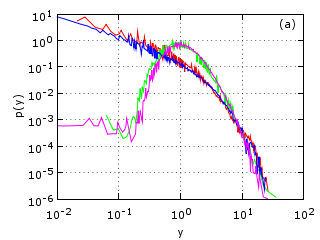
(a)

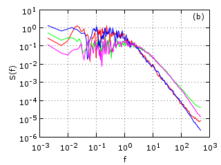
(b)

Figure 1: Agreement between statistical properties of $y$, (a) probability density function and (b) power spectral density, obtained from stochastic (blue and magenta curves) and agent-based (red and green curves) models. Two qualitatively different model phases are shown: red and blue curves correspond to herding dominant model phase ($\sigma_{1}=\sigma_{2}=0.2$, $h=5$), while green and magenta curves correspond to individual behavior dominant model phase ($\sigma_{1}=\sigma_{2}=16$, $h=5$).

Note that the above derivation, and thus, the final equations, does not change even if $\sigma_{1}$, $\sigma_{2}$ or $h$ are functions of $x$ or $y$. Thus, one can further study the possibilities of the model by checking different scenarios of $\sigma_{1}$, $\sigma_{2}$ or $h$ being functions of $x$ or $y$. Nevertheless, the most natural way is to introduce a custom function $\tau(y)$ as inter-event time. In such case the switching probabilities above can be interpreted as probability fluxes per time unit. And thus, one can divide the aforementioned constants by $\tau(y)$. We have chosen the case of

$$\mathrm{d}y=\left(\sigma_{1}+y\frac{2h-\sigma_{2}}{\tau(y)}\right)(1+y)\mathrm{d}t+\sqrt{\frac{2hy}{\tau(y)}}(1+y)\mathrm{d}W,$$ (14)

as nonlinear SDE driving statistics of return in financial market. We did not devide $\sigma_{1}$ by $\tau(y)$ on purpose as one could argue that individual behavior of fundamentalist trader does not depend on the observed returns.

In Fig. 2, we have shown statistical properties of the stochastic model (14) with different $\tau(y)$ scenarios in use.

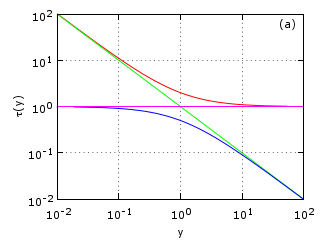
(a)

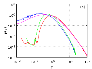
(b)

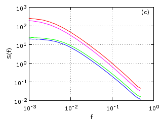
(c)

Figure 2: Statistical properties, probability density functions (sub-figure (b)) and power spectral density (sub-figure (c)), obtained while solving (14) with different $\tau(y)$ scenarios (sub-figure (a)) being in use. Model parameters were set as follows: $\sigma_{1}=\sigma_{2}=0.009$, $h_{0}=0.003$.

Note that while obtained stochastic model appears to be too crude to reproduce statistical properties of financial markets in such details as our stochastic model [2] based on empirical analyzes, it contains long range power-law statistics of return. Obtained equations are very similar to some general stochastic models of the financial markets [14, 17] and thus, in future development might be able to serve as microscopic justification for them and maybe for our more sophisticated modeling [2].

III Two treatments of the Bass Diffusion model

The Bass model introduces a differential equation for the diffusion rate of new products or technologies [9]

$$\frac{\mathrm{d}N(t)}{\mathrm{d}t} = [M-N(t)][p+\frac{q}{M}N(t)],$$ (15)

$$N(0) = 0.$$ (16)

where $N(t)$ denotes the number of product users at time $t$; $M$ is a market potential (number of potential users), $p$ is the coefficient of innovation, the likelihood of an individual to adopt the product due to influence by the commercials or similar external sources, $q$ is the coefficient of imitation, a measure of likelihood that an individual will adopt the product due to influence by other people who already adopted the product. This nonlinear differential equation serves as a macroscopic description of new product adoption by customers widely used in business planning [10].

Another approach to the same problem is related with agent based modeling of product adoption by individual users, or agents. The diffusion process is simulated by computers, where individual decisions of adoption occur with specific adoption probability affected by the other individuals in the neighborhood. It is easy to show that Bass diffusion process is a specific case of Kirman’s herding model [3]. Indeed, lets define $x(t)$ as $x(t)=N(t)/M$ and in analogy with Kirman’s model probability that new user will adopt the product as

$$\pi^{+}(x)=(1-x)\left(\frac{\sigma_{1}}{M}+\frac{h}{M}x\right).$$ (17)

In the case of Bass diffusion process is of one direction and $\pi^{-}(x)=0$. Note that we assume an extensive herding in equation (17) as only in this case the stochastic term in corresponding Langevin equation vanishes with $M\rightarrow\infty$. Then the functions defining the macroscopic system description are as follows

$$A(x) = M\pi^{+}(x)=(1-x)\left(\sigma_{1}+hx\right),$$ (18)

$$D(x) = \pi^{+}(x)=\frac{(1-x)}{M}\left(\sigma_{1}+hx\right).$$ (19)

In the limit $M\rightarrow\infty$ one gets Bass diffusion equation (15) with $p=\sigma_{1}$ and $q=h$ instead of Langevin equation. This proofs that Bass diffusion is a special case of Kirman’s herding model. Though this simple relation looks straightforward, we derive it and confirm by numerical simulations in fairly original way.

In Figure 3 we demonstrate the correspondence between macroscopic and microscopic Bass diffusion description. Agent based and continuous descriptions of product adoption $\Delta N$ per time interval $\Delta t$ converge when number of potential users $M$ or time interval $\Delta t$ increase.

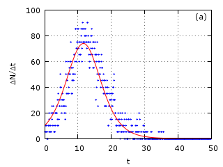
(a)

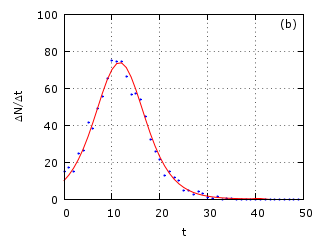
(b)

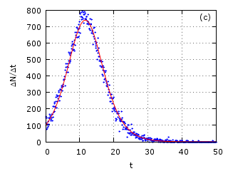
(c)

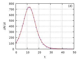
(d)

Figure 3: Comparison of Bass diffusion, $\Delta N/\Delta t$ versus $t$, in macroscopic description (red line) and agent based model (blue points) shows convergence when time interval $\Delta t$ or number of potential users $M$ are increasing. (a) $M=1000$, $\Delta t=0.1$; (b) $M=1000$, $\Delta t=1$; (c) $M=10000$, $\Delta t=0.1$; (d) $M=10000$, $\Delta t=1$. Other parameters are as follows $p=0.01$, $q=0.275$.

One of the goals of developing these models on the web site [11] was to provide theoretical background of Bass diffusion model and practical steps how such computer simulations can be created even with limited IT knowledge and then used for practical purposes. Thus, we target small and medium enterprises to encourage them to use modern computer simulation tools for business planning and other purposes.

Computer models published at the [11] provide a relatively easy starting point to get acquainted with computer simulation and enables portal visitors to use these computer models interactively, running them directly in a window of web browser, changing parameters and observing results. This significantly increases accessibility and dissemination of these simulations.

IV Conclusions and future work

Reasoning of stochastic models of complex systems by the microscopic interactions of agents is still a challenge for researchers. Only very general models such as Kirman’s herding model in ant colony or Bass diffusion model for new product adoption have well established agent based versions and can be described by stochastic or ordinary differential equations. There are many different attempts of microscopic modeling in more sophisticated systems, such as financial markets or other social systems, intended to reproduce the same empirically defined properties. The ambiguity of microscopic description in complex systems is an objective obstacle for quantitative modeling. Simple enough agent based models with established or expected corresponding macroscopic description are indispensable in modeling of more sophisticated systems. In this contribution we discussed various extensions and applications of Kirman’s herding model.

First of all, we modify Kirman’s model introducing interevent time $\tau(y)$ or trading activity $1/\tau(y)$ as functions of driving return $y$. This produces the feedback from macroscopic variables on the rate of microscopic processes and strong nonlinearity in stochastic differential equations responsible for the long range power-law statics of financial variables. We do expect further development of this approach introducing the mood of chartists as independent agent based process.

One more outcome of Kirman’s herding behavior of agents is one direction process - Bass diffusion. This simple example of correspondence between very well established microscopic and macroscopic modeling becomes valuable for further description of diffusion in social systems. Models presented on the interactive web site [6] have to facilitate further extensive use of computer modeling in economics, business and education.

References

- [1] M. Waldrop, Complexity: The emerging order at the edge of order and chaos. New York: Simon & Schuster, 1992.
- [2] V. Gontis, J. Ruseckas, and A. Kononovicius, “A non-linear double stochastic model of return in financial markets,” in Stochastic Control, C. Myers, Ed. Scyio, 2010, pp. 559–580.
- [3] A. Kirman, “Ants, rationality, and recruitment,” Quarterly Journal of Economics, vol. 108, pp. 137–156, 1993.
- [4] S. Alfarano, T. Lux, and F. Wagner, “Estimation of agent-based models: The case of an asymmetric herding model,” Computational Economics, vol. 26, no. 1, pp. 19–49, 2005.
- [5] ——, “Time variation of higher moments in a financial market with heterogeneous agents: An analytical approach,” Journal of Economic Dynamics and Control, vol. 32, no. 1, pp. 101–136, 2008.
- [6] V. Gontis, V. Daniūnas, and A. Kononovičius, “Physics of risk,” Web site: http://mokslasplius.lt/rizikos-fizika/en.
- [7] A. Kononovičius and V. Gontis, “Kirman’s ant colony model,” Web page: http://mokslasplius.lt/rizikos-fizika/en/agent-based-models/kirman-ants.
- [8] ——, “Stochastic ant colony model,” Web page: http://mokslasplius.lt/rizikos-fizika/en/stochastic-models/stochastic-ant-colony-model.
- [9] F. M. Bass, “A new product growth model for consumer durables,” Management Science, vol. 15, pp. 215–227, 1969.
- [10] V. Mahajan, E. Muller, and F. M. Bass, “New-product diffusion models,” in Handbooks in Operations Research and Management Science, G. L. L. J. Eliashberg, Ed. Amsterdam: North Holland, 1993, vol. 5: Marketing, pp. 349–408.
- [11] V. Daniūnas, “Verslo modeliai,” Section on web site: http://mokslasplius.lt/rizikos-fizika/business.
- [12] Oracle Corporation, “java.com: Java + you,” Web site: http://www.java.com/en/.
- [13] X. Technologies, “Anylogic – multi-paradigm simulation software,” Web site: http://www.xjtek.com/anylogic, 2011.
- [14] J. Ruseckas and B. Kaulakys, “1/f noise from nonlinear stochastic differential equations,” Physical Review E, vol. 81, p. 031105, 2010.
- [15] N. G. van Kampen, Stochastic process in Physics and Chemistry. Amsterdam: North Holland, 1992.
- [16] C. W. Gardiner, Handbook of Stochastic Methods. Berlin: Springer, 1997.
- [17] S. Reimann, V. Gontis, and M. Alaburda, “Interplay between positive feedbacks in the generalized CEV process,” Physica A, vol. 390, no. 8, pp. 1393–1401, 2011.