Chapter 26 Enumeration of maps

J. Bouttier
 
Institut de Physique Théorique, CEA Saclay,
F-91191 Gif-sur-Yvette Cedex, France

Abstract

This chapter is devoted to the connection between random matrices and maps, i.e graphs drawn on surfaces. We concentrate on the one-matrix model and explain how it encodes and allows to solve a map enumeration problem.

26.1 Introduction

Maps are fundamental objects in combinatorics and graph theory, originally introduced by Tutte in his series of “census” papers [Tut62a, Tut62b, Tut62c, Tut63]. Their connection to random matrix theory was pioneered in the seminal paper titled “Planar diagrams” by Brézin, Itzykson, Parisi and Zuber [Bre78] building on an original idea of ’t Hooft [Hoo74]. In parallel with the idea that planar diagrams (i.e maps) form a natural discretization for the random surfaces appearing in 2D quantum gravity (see chapter 30), this led to huge developments in physics among which some highlights are the solution by Kazakov [Kaz86] of the Ising model on dynamical random planar lattices (i.e maps) then used as a check for the Knizhnik-Polyakov-Zamolodchikov relations [Kni88].

Matrix models, or more precisely matrix integrals, are efficient tools to address map enumeration problems, and complement other techniques which have their roots in combinatorics, such as Tutte’s original recursive decomposition or the bijective approach. Despite the fact that these techniques originate from different communities, it is undoubtable that they are intimately connected. For instance, it was recognized that the loop equations for matrix models correspond to Tutte’s equations [Eyn06], while the knowledge of the matrix model result proved instrumental in finding a bijective proof [Bou02b] for a fundamental result of map enumeration [Ben94].

In this chapter, we present an introduction to the method of matrix integrals for map enumeration. To keep a clear example in mind, we concentrate on the problem considered in [Ben94, Bou02b] of counting the number of planar maps with a prescribed degree distribution, though we mention a number of possible generalizations of the results encountered on the way. Of course many other problems can be addressed, see for instance chapter 30 for a review of models of statistical physics on discrete random surfaces (i.e maps) which can be solved either exactly or asymptotically using matrix integrals.

This chapter is organized as follows. In section 26.2, we introduce maps and related objects. In section 26.3, we discuss the connection itself between matrix integrals and maps: we focus on the Hermitian one-matrix model with a polynomial potential, and explain how the formal expansion of its free energy around a Gaussian point (quadratic potential) can be represented by diagrams identifiable with maps. In section 26.4, we show how techniques of random matrix theory introduced in previous chapters allow to deduce the solution of the map enumeration problem under consideration. We conclude in section 26.5 by explaining how to translate the matrix model result into a bijective proof.

26.2 Maps: definitions

Colloquially, maps are “graphs drawn on a surface”. The purpose of this section is to make this definition more precise. We recall the basic definitions related to graphs in subsection 26.2.1, before defining maps as graphs embedded into surfaces in subsection 26.2.2. Subsection 26.2.3 is devoted to a coding of maps by pairs of permutations, which will be useful for the following section.

26.2.1 Graphs

A graph is defined by the data of its vertices, its edges, and their incidence relations. Saying that a vertex is incident to an edge simply means that it is one of its extremities, hence each edge is incident to two vertices. Actually, we allow for the two extremities of an edge to be the same vertex, in which case the edge is called a loop. Moreover several edges may have the same two extremities, in which case they are called multiple edges. A graph without loops and multiple edges is said to be simple. (In other terminologies, graphs are always simple and multigraphs refer to the ones containing loops and multiple edges.) A graph is connected if it is not possible to split its set of edges into two or more non-empty subsets in such a way that no edge is incident to vertices from different subsets. The degree of a vertex is the number of edges incident to it, counted with multiplicity (i.e a loop is counted twice).

26.2.2 Maps as embedded graphs

Figure 26.1: Several cellular embeddings of a same graph into the sphere (drawn in the plane by stereographic projection), where half-edges are labelled from 1 to 10. (a) and (b) differ only by a simple deformation. (c) is obtained by choosing another pole for the projection. Thus (a), (b) and (c) represent the same planar map encoded by the permutations $\sigma=(1\,2)(3\,4\,5)(6\,7\,8\,9)(10)$ and $\alpha=(1\,3)(2\,7)(4\,6)(5\,9)(8\,10)$. (d) represents a different map, encoded by the permutations $\sigma^{\prime}=\sigma\circ(8\,9)$ and $\alpha^{\prime}=\alpha$. Their inequivalence may be checked by comparing the face degrees or noting that $\sigma\circ\alpha$ is not conjugate to $\sigma^{\prime}\circ\alpha^{\prime}$.

The surfaces we consider here are supposed to be compact, connected, orientable and without boundary. It is well-known that such surfaces are characterized, up to homeomorphism, by a unique nonnegative integer called the genus, the sphere having genus 0.

An embedding of a graph into a surface is a function associating each vertex with a point of the surface and each edge with a simple open arc, in such a way that the images of distinct graph elements (vertices and edges) are disjoint and incidence relations are preserved (i.e the extremities of the arc associated with an edge are the points associated with its incident vertices). The embedding is cellular if the connected components of the complementary of the embedded graph are simply connected. In that case, these are called the faces and we extend the incidence relations by saying that a face is incident to the vertices and edges on its boundary. Each edge is incident to two faces (which might be equal) and the degree of a face is the number of edges incident to it (counted with multiplicity). It is not difficult to see that the existence of a cellular embedding requires the graph to be connected (for otherwise, graph components would be separated by non-contractible loops).

Maps are cellular embeddings of graphs considered up to continuous deformation, i.e up to an homeomorphism of the target surface. Clearly such a continuous deformation preserves the incidence relations between vertices, edges and faces. It also preserves the genus of the target surface, hence it makes sense to speak about the genus of a map. A planar map is a map of genus 0. In all rigor, this notion should not be confused with that of planar graph, which is a graph having a least one embedding into the sphere. Figure 26.1 shows a few cellular embeddings of a same (planar) graph into the sphere (drawn in the plane by stereographic projection): the first three are equivalent to each other, but not to the fourth (which might immediately be seen by comparing the face degrees). Let us conclude this section by stating the following well-known result.

Theorem 1 (Euler characteristic formula).

In a map of genus $g$, we have

$$\#\{\mathrm{vertices}\}-\#\{\mathrm{edges}\}+\#\{\mathrm{faces}\}=2-2g.$$ (26.2.1)

This quantity is the Euler characteristic $\chi$ of the map.

In the planar case $g=0$, the formula is also called the Euler relation.

26.2.3 Combinatorial maps

As discussed above, a map contains more data than a graph, and one may wonder what is the missing data. It turns out that the embedding into an oriented surface amounts to defining a cyclic order on the edges incident to a vertex. More precisely, as we allow for loops, it is better to consider half-edges, each of them being incident to exactly one vertex. Let us label the half-edges by distinct consecutive integers $1,\ldots,2m$ (where $m$ is the number of edges) in an arbitrary manner. Given a half-edge $i$, let $\alpha(i)$ be the other half of the same edge, and let $\sigma(i)$ be the half-edge encountered after $i$ when turning counterclockwise around its incident vertex (see again Figure 26.1 for an example with $m=5$). It is easily seen that $\sigma$ and $\alpha$ are permutations of $\{1,\ldots,2m\}$, which furthermore satisfy the following properties:

• $\alpha$ is an involution without fixed point,

• the subgroup of the permutation group generated by $\sigma$ and $\alpha$ acts transitively on $\{1,\ldots,2m\}$.

The latter property simply expresses that the underlying graph is necessarily connected. The subgroup generated by $\alpha$ and $\sigma$ is called the cartographic group [Zvo95].

These permutations fully characterize the map. Actually, a pair of permutations ($\sigma,\alpha$) satisfying properties (A) and (B) is called a labelled combinatorial map and there is a one-to-one correspondence between maps (as defined in the previous section) with labelled half-edges and labelled combinatorial maps. In this correspondence, the vertices are naturally associated with the cycles of $\sigma$, the edges with the cycles of $\alpha$ and the faces with the cycles of $\sigma\circ\alpha$. At this stage one may have noticed that vertices and faces play a symmetric role, indeed $(\sigma\circ\alpha,\alpha)$ is also a labelled combinatorial map corresponding to the dual map. Degrees are given the length of the corresponding cycles, and the Euler characteristic is given by

$$\chi(\sigma,\alpha)=c(\sigma)-c(\alpha)+c(\sigma\circ\alpha)$$ (26.2.2)

where $c(\cdot)$ denotes the number of cycles.

Our coding of maps via pairs of permutations depends on an arbitrary labelling of the half-edges, which might seem unsatisfactory. We shall identify configurations differing by a relabelling, and it easily seen that this amounts to identifying $(\sigma,\alpha)$ to all $(\rho\circ\sigma\circ\rho^{-1},\rho\circ\alpha\circ\rho^{-1})$ where $\rho$ is an arbitrary permutation of $\{1,\ldots,2m\}$. These equivalence classes are in one-to-one correspondence with unlabeled maps. This distinction has some consequences for enumeration: for instance the number of labelled maps with $m$ edges is not equal to $(2m)!$ times the number of unlabeled maps, because some equivalence classes have fewer than $(2m)!$ elements (due to symmetries). By the orbit-stabilizer theorem, the number of elements in the class of $(\sigma,\alpha)$ is $(2m)!/\Gamma(\sigma,\alpha)$ where $\Gamma(\sigma,\alpha)$ is the number of permutations $\rho$ such that $\sigma=\rho\circ\sigma\circ\rho^{-1}$ and $\alpha=\rho\circ\alpha\circ\rho^{-1}$ (such $\rho$ is an automorphism). $\Gamma(\sigma,\alpha)$ is often called the “symmetry factor” in the literature, though it is seldom properly defined.

As we shall see in the next section, matrix integrals are naturally related to labelled maps. Enumerating unlabeled maps is a harder problem as it requires classifying their possible symmetries, which is beyond the scope of this text. The distinction is circumvented when considering rooted maps i.e maps with a distinguished half-edge (often represented as a marked oriented edge): such maps have no non-trivial automorphism hence the enumeration problem is equivalent in the labelled and unlabeled case. Most enumeration results in the literature deal with rooted maps. Furthermore maps of large size are “almost surely” asymmetric, so the distinction is irrelevant in this context.

26.3 From matrix integrals to maps

In this section, we return to random matrices in order to present their connection with maps. We will concentrate on the so-called one-matrix model (though we will allude to its generalizations): maps appear as diagrams representing the expansion of its partition function around a Gaussian point. Our goal is to explain this construction in some detail, as this might be also useful for the comprehension of other chapters.

This section is organized as follows. Subsection 26.3.1 provides the definitions and the main statement (Theorem 2) of the topological expansion in the one-matrix model. The following subsections are devoted to its derivation and generalizations. Subsection 26.3.2 discusses Wick’s theorem for Gaussian matrix models. Subsection 26.3.3 introduces ab initio the diagrammatic expansion of the one-matrix model. Subsection 26.3.4 formalizes this computation and shows its natural relation with combinatorial maps. Subsection 26.3.5 finally presents a few generalizations of the one-matrix model.

26.3.1 The one-matrix model

We consider the model of a Hermitian random matrix in a polynomial potential, often called simply the one-matrix model, which has been already discussed in previous chapters. Different notations and conventions exist, for the purposes of this chapter we define its partition function as

$$\Xi_{N}(t,V)=\frac{\int e^{N\operatorname{Tr}\left(-M^{2}/(2t)+V(M)\right)}\,dM}{\int e^{-N\operatorname{Tr}M^{2}/(2t)}\,dM}$$ (26.3.1)

where $dM$ is the Lebesgue measure over the space of Hermitian matrices, and $V$ stands for a “perturbation” of the form

$$V(x)\equiv\sum_{n=1}^{\infty}\frac{v_{n}}{n}x^{n}.$$ (26.3.2)

Here we shall consider the coefficients $v_{n}$ as formal variables hence, rather than a polynomial, $V$ is a formal power series in $x$ and the $v_{n}$. In this sense, a more proper definition of the partition function $\Xi_{N}(t,V)$ is

$$\Xi_{N}(t,V)=\left\langle e^{N\operatorname{Tr}V(M)}\right\rangle$$ (26.3.3)

where $\langle\cdot\rangle$ denotes the expectation value with respect to the Gaussian measure proportional to $e^{-N\operatorname{Tr}M^{2}/(2t)}\,dM$, acting coefficient-wise on $e^{N\operatorname{Tr}V(M)}$ viewed as a formal power series in the $v_{n}$ whose coefficients are polynomials in the matrix elements. In other words, the matrix integral in (26.3.1) must be understood in the “formal” sense of chapter 16. We define furthermore the free energy by

$$F_{N}(t,V)=\log\Xi_{N}(t,V).$$ (26.3.4)

The main purpose of this section is to establish the following theorem, which is essentially a formalization of ideas present in [Bre78, Hoo74].

Theorem 2 (Topological expansion).

The free energy of the one-matrix model has the “topological” expansion

$$F_{N}(t,V)=\sum_{g=0}^{\infty}N^{2-2g}F^{(g)}(t,V)$$ (26.3.5)

where $F^{(g)}(t,V)$ is equal to the exponential generating function for labelled maps of genus $g$ with a weight $t$ per edge and, for all $n\geq 1$, a weight $v_{n}$ per vertex of degree $n$.

Corollary.

The quantity

$$E^{(g)}(t,V)=2t\frac{\partial F^{(g)}(t,V)}{\partial t}$$ (26.3.6)

is the generating function for rooted maps (i.e maps with a distinguished half-edge) of genus $g$. Similarly $nv_{n}\frac{\partial F^{(g)}(t,V)}{\partial v_{n}}$ corresponds to rooted maps of genus $g$ whose root vertex (i.e the vertex incident to the distinguished half-edge) has degree $n$. Maps with several marked edges or vertices are obtained by taking multiple derivatives.

We recall that, from the discussion of section 26.2.3, a labelled map is a map whose half-edges are labelled $\{1,\ldots,2m\}$ where $m$ is the number of edges. Hence by exponential generating function for labelled maps we mean

$$F^{(g)}(t,V)=\sum_{m=0}^{\infty}\frac{t^{m}}{(2m)!}F^{(g,m)}(V)$$ (26.3.7)

where $F^{(g,m)}(V)$ is the (finite) sum over labelled maps of genus $g$ with $m$ edges of the product of vertex weights. If we want to reduce $F^{(g,m)}(V)$ to a sum over unlabeled maps instead, then the multiplicity of an individual unlabeled map is $(2m)!/\Gamma$, where $\Gamma$ is its number of automorphisms. The $(2m)!$ cancels the denominator in (26.3.7) leading to an ordinary generating function, where however the weight $1/\Gamma$ has to be kept. It differs from the “true” generating function for unlabeled maps where this weight is absent. For rooted maps there is no difference since $\Gamma=1$ for all of them: we simply refer to the generating function for rooted maps without specifying between exponential/labelled and ordinary/unlabeled.

$F^{(0)}(t,V)$ is called the planar free energy. Informally, it is “dominant” in the large $N$ limit. Actually, equation (26.3.5) makes sense as a sum of formal power series (at a given order in $t$, only a finite number of terms contribute).

26.3.2 Gaussian model, Wick theorem

In order to derive theorem 2, we first consider the Gaussian measure

$$\left(\frac{N}{2\pi t}\right)^{N^{2}/2}\,e^{-N\operatorname{Tr}M^{2}/(2t)}\,dM$$ (26.3.8)

where $dM$ is the Lebesgue (translation-invariant) measure over the set of Hermitian matrices of size $N$. It is easily seen that the matrix elements are centered jointly Gaussian random variables, with covariance

$$\langle M_{ij}M_{kl}\rangle=\delta_{il}\delta_{jk}\frac{t}{N}.$$ (26.3.9)

More generally, the expectation value of the product of arbitrarily many matrix elements is given via Wick’s theorem (generally valid for any Gaussian measure). This classical result can be stated as follows.

Theorem 3 (Wick’s theorem for matrix integrals).

The expectation value of the product of an arbitrary number of matrix elements is equal to the sum, over all possible pairwise matchings of the matrix elements, of the product of pairwise covariance.

For instance, for $4$ matrix elements we have

$$\begin{split}\langle M_{i_{1}j_{1}}M_{i_{2}j_{2}}M_{i_{3}j_{3}}M_{i_{4}j_{4}}\rangle&=\langle M_{i_{1}j_{1}}M_{i_{2}j_{2}}\rangle\langle M_{i_{3}j_{3}}M_{i_{4}j_{4}}\rangle\\ &+\langle M_{i_{1}j_{1}}M_{i_{3}j_{3}}\rangle\langle M_{i_{2}j_{2}}M_{i_{4}j_{4}}\rangle\\ &+\langle M_{i_{1}j_{1}}M_{i_{4}j_{4}}\rangle\langle M_{i_{2}j_{2}}M_{i_{3}j_{3}}\rangle.\end{split}$$ (26.3.10)

Clearly, for an odd number of elements the expectation value vanishes by parity, while for an even number $2n$ of elements the sum involves $(2n-1)!!=(2n-1)(2n-3)\cdots 5\cdot 3\cdot 1$ terms.

Let us note immediately that these results extend easily to a Gaussian model of $K$ random Hermitian matrices $M^{(1)},\ldots,M^{(K)}$ of same size $N$, with measure

$$\left(\frac{N^{K}\det Q}{2^{K}\pi^{K}}\right)^{N^{2}/2}\exp\left(-\frac{N}{2}\sum_{a,b=1}^{K}Q_{ab}\operatorname{Tr}M^{(a)}M^{(b)}\right)\,dM^{(1)}\,\cdots\,dM^{(K)}$$ (26.3.11)

where $Q$ is a $K\times K$ real symmetric matrix. The covariance of two matrix elements is

$$\langle M_{ij}^{(a)}M_{kl}^{(b)}\rangle=\delta_{il}\delta_{jk}\frac{(Q^{-1})_{ab}}{N}.$$ (26.3.12)

and, taking the extra index into account, Wick’s theorem still applies, for instance

$$\begin{split}\langle M_{i_{1}j_{1}}^{(a_{1})}M_{i_{2}j_{2}}^{(a_{2})}M_{i_{3}j_{3}}^{(a_{3})}M_{i_{4}j_{4}}^{(a_{4})}\rangle&=\langle M_{i_{1}j_{1}}^{(a_{1})}M_{i_{2}j_{2}}^{(a_{2})}\rangle\langle M_{i_{3}j_{3}}^{(a_{3})}M_{i_{4}j_{4}}^{(a_{4})}\rangle\\ &+\langle M_{i_{1}j_{1}}^{(a_{1})}M_{i_{3}j_{3}}^{(a_{3})}\rangle\langle M_{i_{2}j_{2}}^{(a_{2})}M_{i_{4}j_{4}}^{(a_{4})}\rangle\\ &+\langle M_{i_{1}j_{1}}^{(a_{1})}M_{i_{4}j_{4}}^{(a_{4})}\rangle\langle M_{i_{2}j_{2}}^{(a_{2})}M_{i_{3}j_{3}}^{(a_{3})}\rangle.\end{split}$$ (26.3.13)

26.3.3 Diagrammatics of the one-matrix model: a first approach

We now return to the partition function (26.3.3), which is a formal power series in the variables $v_{n}$. If $\mathitbf{k}=(k_{n})_{n\geq 1}$ denotes a family of nonnegative integers with finite support, the coefficient of the monomial $\mathitbf{v}^{\mathitbf{k}}=\prod_{n=1}^{\infty}v_{n}^{k_{n}}$ in $\Xi_{N}(t,V)$ reads

$$\left[\mathitbf{v}^{\mathitbf{k}}\right]\,\Xi_{N}(t,V)=\left\langle\prod_{n=1}^{\infty}\frac{\left(N\operatorname{Tr}M^{n}\right)^{k_{n}}}{n^{k_{n}}k_{n}!}\right\rangle.$$ (26.3.14)

Inside this expression, each trace $\operatorname{Tr}M^{n}$ can be rewritten as a sum of product of $n$ elements of $M$, for instance

$$\operatorname{Tr}M^{3}=\sum_{i,j,k=1}^{N}M_{ij}M_{jk}M_{ki}.$$ (26.3.15)

hence (26.3.14) may itself be rewritten as the expectation value of a finite linear combination of products of elements of $M$, to be evaluated via Wick’s theorem.

Figure 26.2: Elements constituting the Feynman diagrams for the Hermitian one-matrix model: (a) a leg representing a matrix element, (b) a 3-leg vertex representing a term in $\operatorname{Tr}M^{3}$, (c) two paired elements forming an edge.

We may represent graphically the factors appearing in this decomposition as follows (see also Figure 26.2):

• Each matrix element $M_{ij}$ is represented as a double line originating from a point, forming a leg. The lines are oriented in opposite directions (incoming and outgoing) and “carry” respectively an index $i$ and $j$.

• Each product of matrix elements appearing in the expansion of $\operatorname{Tr}M^{n}$ is represented as $n$ legs incident to the same point forming a vertex. The legs are cyclically ordered around the vertex so that each incoming line is connected to the outgoing line of the consecutive leg, and carries the same index. This directly translates the pattern of indices obtained when writing a trace as product of matrix elements. For instance, for $n=3$ the decomposition (26.3.15) yields the vertex shown on Figure 26.2(b), where each index $i$, $j$, or $k$ takes $N$ possible values.

• Wick’s theorem states that the expectation value of a product of matrix elements is obtained by matching them pairwise in all possible manners, and taking the corresponding product of covariances. A pair of matched elements is represented by linking the corresponding legs, forming an edge. More precisely, the incoming line of the one leg is connected to the outgoing line of the other leg, and carries the same index. This translates relation (26.3.9): if the connected lines do not carry the same index, then the covariance vanishes hence the matching does not contribute to the expectation value.

Globally, the factors appearing in (26.3.14) form a collection of $k=\sum k_{n}$ vertices, consisting of $k_{n}$ $n$-leg vertices for all $n\geq 1$. The expectation value is obtained by matching the $\sum nk_{n}$ legs, i.e merging them pairwise into edges, in all possible manners. Hence, the quantity (26.3.14) is expressed as a sum over all diagrams built out of these vertices and edges, which are sometimes called fatgraphs or ribbon graphs in the literature. By the rules discussed above, the index lines that are merged together must carry the same index, and they form closed oriented cycles. There is clearly a finite number of diagrams, since there are $(\sum nk_{n})!!$ ways to merge the legs (in particular, if the number of legs is odd, there are no such diagrams, and correspondingly the expectation value vanishes). It remains to determine what is the contribution of an individual diagram. Because of relation (26.3.9), each of the $m=\sum nk_{n}/2$ edges produces a factor $1/\lambda=t/N$. Hence all diagrams will have the same contribution $t^{m}N^{k-m}/\prod_{n=1}^{\infty}n^{k_{n}}k_{n}!$, taking into account the extra factors present in (26.3.14). Evaluating this matrix integral amounts to counting the number of such diagrams.

Figure 26.3: The three possible types of diagram appearing in the expansion of $\langle\operatorname{Tr}M^{3}\cdot\operatorname{Tr}M^{3}\rangle$.

However, the sum involves many “equivalent” diagrams, i.e diagrams which differ only by the choice of line indices or which have the same “shape”. For instance, Figure 26.3 displays the three possible types of diagrams obtained when expanding $\langle\operatorname{Tr}M^{3}\cdot\operatorname{Tr}M^{3}\rangle$ (in this example, all three diagrams are connected but this is not true in general). Clearly, we may forget about the line indices by counting each index-less diagram with a multiplicity $N^{\ell}$, where $\ell$ is the number of cycles of index lines. In our example, we have $\ell=3$ for the first two diagrams while $\ell=1$ for the third. Evaluating the shape multiplicity is slightly more subtle, and we leave its general discussion to the next subsection. It is not difficult to do the computation for the diagrams of Figure 26.3, which yields the respective shape multiplicities 9, 3 and 3, and gathering the various factors we arrive at

$$\langle\operatorname{Tr}M^{3}\cdot\operatorname{Tr}M^{3}\rangle=(9N^{3}+3N^{3}+3N)(t/N)^{3}=\left(12+\frac{3}{N^{2}}\right)t^{3}.$$ (26.3.16)

Generally, as mentioned above, the coefficient (26.3.14) will correspond to a sum over all (not necessarily connected) diagrams made out of $k_{n}$ vertices with $n$ legs for all $n$. The partition function $\Xi_{N}(t,V)$ is then obtained by summing over all $k_{n}$’s, attaching a weight $v_{n}$ per $n$-leg vertex, leading to the generating function for all diagrams (possibly empty or disconnected). Then $F_{N}(t,V)=\log\Xi_{N}(t,V)$ is the generating function for connected diagrams, as it is well-known. In $\Xi_{N}(t,V)$ as well as in $F_{N}(t,V)$, the exponent of $N$ in the contribution of a diagram is equal to the number of vertices minus the number of edges plus the number of index lines.

Figure 26.4: The maps corresponding to the diagrams of figure 26.3: the first two have genus 0, the third genus 1.

At this stage, it might be rather clear that our (connected) diagrams are nothing but maps in disguise (see figure 26.4). Indeed they are graphs endowed with a cyclic order of half-edges (legs) around the vertices, which is a characterization of maps as discussed in section 26.2. The cycles of index lines correspond to faces, hence the exponent of $N$ in the contribution of a diagram to $F_{N}(t,V)$ is equal to the Euler characteristic of the corresponding map. This essentially establishes theorem 2.

26.3.4 One-matrix model and combinatorial maps

In this section, we revisit the calculation done above in a more formal manner. The purpose is to show that it naturally involves labelled combinatorial maps, i.e pairs of permutations, as defined in section 26.2.3.

We start from a “classical” formula for enumerating permutations with prescribed cycle lengths. Let $\mathcal{S}_{p}$ denote the set of permutations of $\{1,\ldots,p\}$ and $c_{n}(\sigma)$ denote the number of $n$-cycles in the permutation $\sigma$, $c(\sigma)$ being the total number of cycles. Then the numbers of permutations $\sigma$ in $\mathcal{S}_{p}$ with prescribed values of $c_{n}(\sigma)$ for all $n\geq 1$ are encoded into the exponential multivariate generating function

$$\exp\left(\sum_{n=1}^{\infty}\frac{A_{n}}{n}\right)=\sum_{p=0}^{\infty}\frac{1}{p!}\sum_{\sigma\in\mathcal{S}_{p}}\prod_{n=1}^{\infty}A_{n}^{c_{n}(\sigma)}.$$ (26.3.17)

Here $(A_{n})_{n\geq 1}$ is a family of formal variables. Establishing this formula is a simple exercise in combinatorics [Fla08]: it simply translates the decomposition of a permutation into cycles. We recover $\Xi_{N}(t,V)$ of (26.3.1) on the left-hand side by the substitution

$$A_{n}=Nv_{n}\operatorname{Tr}M^{n}$$ (26.3.18)

and taking the expectation value over the Gaussian random matrix $M$. By this substitution, the $\sigma$ term on the right hand side is, up to a factor independent of $M$, equal to a product of traces which we may rewrite as

$$\prod_{n=1}^{\infty}(\operatorname{Tr}M^{n})^{c_{n}(\sigma)}=\sum_{(i_{1},\ldots,i_{p})\in\{1,\ldots,N\}^{p}}\prod_{q=1}^{p}M_{i_{q}\,i_{\sigma(q)}}.$$ (26.3.19)

Wick’s theorem and relation (26.3.9) yield

$$\left\langle\prod_{q=1}^{p}M_{i_{q}\,i_{\sigma(q)}}\right\rangle=\left(\frac{t}{N}\right)^{p/2}\sum_{\alpha\in\mathcal{I}_{p}}\prod_{q=1}^{p}\delta_{i_{q}\,i_{\sigma(\alpha(q))}}$$ (26.3.20)

where $\mathcal{I}_{p}\subset\mathcal{S}_{p}$ is the set of involutions without fixed point (aka pairwise matchings) of $\{1,\ldots,p\}$, which is empty for $p$ odd. We then observe that the product on the right hand side of (26.3.20) is equal to 1 if the index $i_{q}$ is constant over the cycles of the permutation $\sigma\circ\alpha$, otherwise it is 0. Therefore, when summing over all values of $(i_{1},\ldots,i_{p})$, we find

$$\left\langle\prod_{n=1}^{\infty}(\operatorname{Tr}M^{n})^{c_{n}(\sigma)}\right\rangle=\left(\frac{t}{N}\right)^{p/2}\sum_{\alpha\in\mathcal{I}_{p}}N^{c(\sigma\circ\alpha)}.$$ (26.3.21)

Plugging into (26.3.17) and (26.3.18) and writing $p=2m=2c(\alpha)$, we arrive at

$$\Xi_{N}(t,V)=\sum_{m=0}^{\infty}\frac{t^{m}}{(2m)!}\sum_{(\sigma,\alpha)\in\mathcal{S}_{2m}\times\mathcal{I}_{2m}}N^{c(\sigma)-c(\alpha)+c(\sigma\circ\alpha)}\prod_{n=1}^{\infty}v_{n}^{c_{n}(\sigma)}.$$ (26.3.22)

We are very close to recognizing a sum over combinatorial maps, with the Euler characteristic (26.2.2) appearing as the exponent of $N$, but we lack the requirement that $\sigma$ and $\alpha$ generate a transitive subgroup. Again, this is implemented by taking the logarithm (in combinatorial terms [Fla08], $\mathcal{S}_{2m}\times\mathcal{I}_{2m}$ is equal to the labelled set construction applied to the class of combinatorial maps – as seen by decomposing $\{1,\ldots,2m\}$ into orbits – and all parameters are inherited, hence $\Xi_{N}(t,V)$ is the exponential of the generating function for combinatorial maps), leading to

$$F_{N}(t,V)=\log\Xi_{N}(t,V)=\sum_{m=0}^{\infty}\frac{t^{m}}{(2m)!}\sum_{(\sigma,\alpha)\in\mathcal{M}_{m}}N^{\chi(\sigma,\alpha)}\prod_{n=1}^{\infty}v_{n}^{c_{n}(\sigma)}$$ (26.3.23)

where $\mathcal{M}_{m}$ is the set of labelled combinatorial maps with $m$ edges. Upon regrouping the maps according to their genus, this yields relation (26.3.7) and formally establishes theorem 2.

26.3.5 Generalization to multi-matrix models

Let us now briefly discuss multi-matrix models. Informally, we consider a “perturbation” of the multi-matrix Gaussian model (26.3.11) by a $U(N)$-invariant potential $N\operatorname{Tr}V(M^{(1)},M^{(2)},\ldots,M^{(K)})$, where $V(x_{1},x_{2},\ldots,x_{K})$ is a “polynomial” in $K$ non-commutative variables. Actually, $V$ shall be viewed as a formal linear combination of monomials in $p$ non-commutative variables $x_{1},x_{2},\ldots,x_{K}$ namely

$$V(x_{1},x_{2},\ldots,x_{K})=\sum_{n=0}^{\infty}\sum_{(a_{1},\ldots,a_{n})\in\{1,\ldots,K\}^{n}}\frac{v(a_{1},\ldots,a_{n})}{n}x_{a_{1}}\cdots x_{a_{n}}$$ (26.3.24)

where the $v(a_{1},\ldots,a_{n})$ are formal variables with the identification $v(a_{2},\ldots,a_{n},a_{1})=v(a_{1},a_{2},\ldots,a_{n})$ (since the trace is invariant by cyclic shifts). The partition function is defined as the expectation value of $e^{N\operatorname{Tr}V(M^{(1)},M^{(2)},\ldots,M^{(K)})}$ under the Gaussian measure (26.3.11), and the free energy as its logarithm. By a simple extension of the arguments of section 26.3.3 (using Wick’s theorem for multi-matrix integrals), the free energy may be written as a sum over maps, whose half-edges now carry one of $K$ “colours” corresponding to the extra index $a=1,\ldots,K$. The formal variable $v(a_{1},\ldots,a_{n})$ is the weight for vertices around which the half-edge colors are $(a_{1},\ldots,a_{n})$ in cyclic order, and $Q^{-1}_{ab}$ is the weight per edge whose halves are colored $a$ and $b$. Furthermore the topological expansion (26.3.5) still holds.

In the particular case

$$V(x_{1},x_{2},\ldots,x_{K})=\sum_{n=1}^{\infty}\sum_{a=1}^{K}\frac{v_{n}^{(a)}}{n}x_{a}^{n},$$ (26.3.25)

all legs incident to a same vertex carry the same colour. The free energy yields the generating function for (labelled) maps of a given genus whose vertices are colored in $K$ colours, with a weight $v_{n}^{(a)}$ per vertex with colour $a$ and degree $n$, and a weight $Q^{-1}_{a,b}$ per edge linking of vertex of colour $a$ to a vertex of colour $b$.

Instances of these models appears in several other chapters. Those corresponding to the form (26.3.25) include the chain matrix model in chapter 16, the Ising and Potts models in chapter 30. Models of the form (26.3.24) but not (26.3.25) include the complex matrix model in chapter 27 (for the diagrammatic expansion, $M$ and $M^{\dagger}$ may be treated as two independent Hermitian matrices, which are represented with outgoing and incoming arrows), the $O(n)$, six-vertex and SOS/ADE models in chapter 30. We particularly emphasize the two-matrix model with free energy

$$\log\frac{\int\,\exp\left(-\frac{N}{t}\operatorname{Tr}M_{1}M_{2}+\sum_{n}\frac{Nv_{n}^{(1)}}{n}\operatorname{Tr}M_{1}^{n}+\sum_{n}\frac{Nv_{n}^{(2)}}{n}\operatorname{Tr}M_{2}^{n}\right)\,dM_{1}\,dM_{2}}{\int\,\exp\left(\frac{N}{t}\operatorname{Tr}M_{1}M_{2}\right)dM_{1}\,dM_{2}\,}$$ (26.3.26)

which yields generating functions for bipartite maps with a weight per vertex depending on degree and colour. It is the most natural generalization of the counting problem addressed with the one-matrix model (recovered by setting $v^{(2)}_{n}=\delta_{n,2}/t$).

Let us finally mention that the diagrammatic expansion for real symmetric matrices corresponds to maps on unoriented surfaces.

26.4 The vertex degree distribution of planar maps

This section is devoted to the enumeration of rooted planar maps with a prescribed vertex degree distribution, i.e with a given number of vertices of each degree. This is equivalent to deriving the generating function for rooted planar maps with a weight $t$ per edge and, for all $n\geq 1$, a weight $v_{n}$ per vertex of degree $n$. By theorem 2 and its corollary, this in turn amounts to computing the derivative with respect to $t$ of the planar free energy of the one-matrix model.

Let us first state the result, in the form given in [Bou02b]. A different form was obtained independently in [Ben94] (without matrices), and a check of their agreement can be found in [Bou06].

Theorem 4.

Let $R,S$ be the formal power series in $t$ and $(v_{n})_{n\geq 1}$ satisfying

$$\begin{split}R&=t+t\sum_{n=1}^{\infty}v_{n}\sum_{j=1}^{\lfloor\frac{n}{2}\rfloor}\frac{(n-1)!}{j!(j-1)!(n-2j)!}R^{j}S^{n-2j}\\ S&=t\sum_{n=1}^{\infty}v_{n}\sum_{j=0}^{\lfloor\frac{n-1}{2}\rfloor}\frac{(n-1)!}{(j!)^{2}(n-2j-1)!}R^{j}S^{n-2j-1}.\end{split}$$ (26.4.1)

Then the generating function of rooted planar maps with a weight $t$ per edge and, for all $n$, a weight $v_{n}$ per vertex of degree $n$ is given by

$$E^{(0)}=\frac{1}{t}\left(R+S^{2}-\sum_{n=1}^{\infty}v_{n}\sum_{j=2}^{\lfloor\frac{n+2}{2}\rfloor}\frac{(2n-3j+2)(n-1)!}{j!(j-2)!(n-2j+2)!}R^{j}S^{n-2j+2}-t\right).$$ (26.4.2)

Remark.

Clearly, $R,S$ are uniquely determined from the requirement that $R=S=0$ for $t=0$. They have a direct combinatorial interpretation: $R$ is the generating function for planar maps with two distinguished vertices of degree 1 (without weights), $S$ is the generating function for planar maps with one distinguished vertex (without weight) of degree 1 and one distinguished face.

Let us mention that the planar free energy $F^{(0)}$ itself has a more complicated expression, involving logarithms.

This section is organized as follows. In subsection (26.4.1) we discuss the main equation describing the planar limit. In subsection (26.4.2) we explain how to solve this equation and derive theorem 4. Finally in subsection (26.4.3) we present a few instances with explicit counting formulas.

26.4.1 Saddle-point, loop, Tutte’s equations

Our goal is to “solve” the one-matrix model in the large $N$ limit, i.e extract the genus 0 contribution in (26.3.5). This problem has already been approached several times in this book (particularly in chapters 14 and 16), let us recall what the “master” equation is. It is an equation is for a quantity called the resolvent in the context of matrix integrals. For our purposes, it is nothing but a generating function for rooted maps involving an extra variable attached to the degree of the root vertex.

More precisely, we define here the planar resolvent as

$$W(z)=\sum_{n=0}^{\infty}\frac{W_{n}}{z^{n+1}}=\sum_{n=0}^{\infty}\frac{n}{z^{n+1}}\frac{\partial F_{n}^{(0)}}{\partial v_{n}}$$ (26.4.3)

where $z$ is a new formal variable and $W_{n}$ is the generating function for rooted (i.e with a distinguished half-edge) planar maps whose root vertex (i.e the vertex incident to the root) has degree $n$, with a weight $t$ per edge and, for all $n$, a weight $v_{n}$ per non-root vertex. By convention we set $W_{0}=1$. In comparison with the corollary of theorem 2 we do not attach a weight to the root vertex.

Then, the planar resolvent satisfies the master equation

$$W(z)^{2}-\left(\frac{z}{t}-V^{\prime}(z)\right)W(z)+P(z)=0$$ (26.4.4)

which is a quadratic equation for $W(z)$ immediately solved into

$$W(z)=\frac{1}{2}\left(\frac{z}{t}-V^{\prime}(z)\pm\sqrt{\left(\frac{z}{t}-V^{\prime}(z)\right)^{2}-4P(z)}\right).$$ (26.4.5)

At this stage $P(z)$ is still an unknown quantity but all derivations of (26.4.4) show that, unlike $W(z)$, $P(z)$ contains only non-negative powers of $z$. Actually, if $V(z)$ is a polynomial of degree $d$ (i.e we set $v_{n}=0$ for $n>d$), then $P(z)$ is a polynomial of degree $d-2$. These remarks are instrumental in solving the equation, as discussed in the next subsection. Let us first briefly review some methods for deriving the master equation.

Saddle-point approximation. The saddle-point approximation is the original “physical” method used in [Bre78]. It consists in treating the partition function (26.3.1) as a “genuine” matrix integral and extracting its analytical large $N$ asymptotics. This is done classically by reducing to an integral over the eigenvalues, then determining the dominant eigenvalue distribution. See chapter 14, sections 1 and 2, for a general discussion of this method. Equation (14.2.6) is nothing but equation (26.4.5) in different notations: the quantities denoted by $F(z)$, $Q(z)$ and $V^{\prime}(z)$ in chapter 14 correspond respectively to $W(z)$, $P(z)$ and $\frac{z}{t}-V^{\prime}(z)$ here.

Loop equations. Loop equations correspond to the Schwinger–Dyson equations of quantum field theory applied in the context of matrix models [Wad81, Mig83], see chapter 16 for a general discussion and application in the context of the one-matrix model. An interesting feature of loop equations is that they provide an easier access to higher genus contributions than the saddle-point approximation. However we are here interested in the planar case for which they are essentially equivalent. Again, equation (16.4.1) is (26.4.4) in different notations: the quantities denoted by $W_{1}^{(0)}(x)$, $P^{(0)}(z)$ and $V^{\prime}(z)$ in chapter 16 correspond respectively to $W(z)$, $P(z)$ and $\frac{z}{t}-V^{\prime}(z)$ here.

Tutte’s recursive decomposition. Tutte’s original approach consists in recursively decomposing rooted maps by “removing” (contracting or deleting) the root edge. It translates into an equation determining their generating function, upon introducing an extra “catalytic” variable in order to make the decomposition bijective. It is now recognized that Tutte’s equations are essentially equivalent to loop equations [Eyn06] despite their very different origin.

Let us explain the recursive decomposition in our setting [Tut68, Bou06]. We consider a rooted planar map whose root degree (i.e the degree of the root vertex) is $n$, and we decompose it as follows.

• If the root edge is a loop (i.e connects the root vertex to itself), then it naturally “splits” the map into two parts, which may be viewed as two rooted planar maps. If there are $i$ half-edges incident to the root vertex on one side (excluding those of the loop), then there are $n-2-i$ on the other side. These are the respective root degrees of the corresponding maps.

• If the root edge is not a loop, then we contract it (and we may canonically pick a new root). If $m$ denotes the degree of the other vertex incident to the root edge in the original map, then the root degree of the contracted map is $n+m-2$.

This decomposition is clearly reversible. Taking into account the weights, it leads to the equation

$$W_{n}=t\sum_{i=0}^{n-2}W_{i}W_{n-2-j}+t\sum_{m=1}^{\infty}v_{m}W_{n+m-2}$$ (26.4.6)

valid for all $n\geq 1$ with the convention $W_{0}=1$. Equation (26.4.4) is deduced using (26.4.3), in particular $P(z)$ is given by

$$P(z)=-\sum_{n=0}^{\infty}\left(\sum_{m=n+2}^{\infty}v_{m}W_{m-2-n}\right)z^{n}.$$ (26.4.7)

26.4.2 One-cut solution

We now turn to the solution of equation (26.4.4). In the context of matrix models, it gives the “one-cut solution” discussed for instance in chapter 14. Here we concentrate on expressing it in combinatorial form. Let us first suppose that $V(z)$ (hence $P(z)$) is a polynomial in $z$. The one-cut solution is obtained by assuming that the polynomial $\Delta(z)=\left(z/t-V^{\prime}(z)\right)^{2}-4P(z)$ appearing under the square root in (26.4.5) has exactly two simple zeroes, say in $a$ and $b$, and only double zeroes elsewhere. This leads to

$$W(z)=\frac{1}{2}\left(\frac{z}{t}-V^{\prime}(z)+G(z)\sqrt{(z-a)(z-b)}\right)$$ (26.4.8)

where $G(z)$ is a polynomial. This assumption is physically justified in the saddle-point picture by saying that the dominant eigenvalue distribution has a support made of a single interval $[a,b]$ (corresponding to the cut of $W(z)$), as a perturbation of Wigner’s semi-circle distribution. Alternatively, a rigorous proof comes via Brown’s lemma [Bro65], which translates the fact that $W(z)$ hence $\sqrt{\Delta(z)}$ are power series without fractional powers, we refer to [Bou06, section 10] for details in the current context. $\sqrt{(z-a)(z-b)}$ must be understood as a Laurent series in $1/z$, i.e $\sqrt{(z-a)(z-b)}=z+\text{(lower powers in $z$)}$.

Now, it turns out that $a,b$ and $G(z)$ in (26.4.8) may be fully determined from the mere condition that $W(z)=1/z+\text{(lower powers in $z$)}$. Indeed, let us rewrite (26.4.8) as

$$\frac{W(z)}{\sqrt{(z-a)(z-b)}}=\frac{1}{2}\left(\frac{\frac{z}{t}-V^{\prime}(z)}{\sqrt{(z-a)(z-b)}}+G(z)\right).$$ (26.4.9)

Then, we first extract the coefficients of $z^{-1}$ and $z^{-2}$ on both sides. On the left hand side, we obtain respectively $0$ and $1$ by the above condition. On the right hand side, $G(z)$ does not contribute since it is a polynomial in $z$. Therefore we arrive at

$$\left.\frac{\frac{z}{t}-V^{\prime}(z)}{\sqrt{(z-a)(z-b)}}\right|_{z^{-1}}=0\qquad\left.\frac{\frac{z}{t}-V^{\prime}(z)}{\sqrt{(z-a)(z-b)}}\right|_{z^{-2}}=2.$$ (26.4.10)

These equations determine $a$ and $b$ in terms of $t$ and $V(z)$. The coefficients may be extracted via a contour integration around $z=\infty$, but a nicer form is obtained by performing a change of variable $z\to u$ given by

$$z=u+S+\frac{R}{u}$$ (26.4.11)

also known as Joukowsky’s transform. $S$ and $R$ are chosen such that $(z-a)(z-b)$ becomes a perfect square namely

$$S=\frac{a+b}{2}\qquad R=\frac{(b-a)^{2}}{16}\qquad(z-a)(z-b)=\left(u-\frac{R}{u}\right)^{2}.$$ (26.4.12)

Then, by this change of variable, relations (26.4.10) yield

$$S=t\left.V^{\prime}\left(u+S+\frac{R}{u}\right)\right|_{u^{0}}\qquad R=t+t\left.V^{\prime}\left(u+S+\frac{R}{u}\right)\right|_{u^{-1}}.$$ (26.4.13)

Upon expanding $V^{\prime}(z)=\sum v_{n}z^{n}$, then extracting the respective coefficients of $u^{0}$ and $u^{-1}$ in $(u+S+R/u)^{k}$ via the multinomial formula, we obtain the equations (26.4.1).

Extracting further coefficients $z^{-3},z^{-4},\ldots$ in (26.4.9) , we may determine step by step the first few $W_{n}$. In particular, $W_{2}$ is, up to a factor, the generating function $E^{(0)}$ for rooted planar maps (without condition on the root vertex), since marking a bivalent vertex is tantamount to marking an edge. A slightly tedious computation yields

$$E^{(0)}=\frac{R+S^{2}-\left.V^{\prime}\left(u+S+\frac{R}{u}\right)\right|_{u^{-3}}-2S\left.V^{\prime}\left(u+S+\frac{R}{u}\right)\right|_{u^{-2}}-t}{t}.$$ (26.4.14)

which can then be put into the form (26.4.2). This establishes theorem 4, upon noting the restriction that $V(z)$ is a polynomial may now be “lifted”: at a given order in $t$, the coefficient of $E^{(0)}$ and the corresponding sum over maps both depend on finitely many $v_{n}$, therefore by suitably truncating $V(z)$ we may establish their equality.

26.4.3 Examples

Tetravalent maps. In the case of a quartic potential $V(x)=x^{4}/4$, the diagrammatic expansion involves only vertices of degree 4, forming 4-regular or tetravalent maps. Equations (26.4.1) and (26.4.2) reduce to

$$E^{(0)}_{4}=\frac{R-R^{3}}{t}\qquad S=0\qquad R=t+3tR^{2}.$$ (26.4.15)

$R$ is given by a particularly simple quadratic equation solved as

$$R=\frac{1-\sqrt{1-12t^{2}}}{6t}=\sum_{k=0}^{\infty}\frac{1}{k+1}\binom{2k}{k}\,3^{k}\,t^{2k+1}$$ (26.4.16)

where we recognize the celebrated Catalan numbers. Substituting into $E^{(0)}_{4}$ we obtain the series expansion

$$E^{(0)}_{4}=\sum_{k=0}^{\infty}\frac{2(2k)!}{k!(k+2)!}\,3^{k}\,t^{2k}$$ (26.4.17)

where we identify the number of rooted planar tetravalent maps with $2k$ edges (hence $k$ vertices). This is the same number as that of (general) rooted planar maps with $k$ edges [Tut63], as seen by Tutte’s equivalence, and that of rooted planar quadrangulations (i.e maps with only faces of degree 4) with $k$ faces, as seen by duality.

Trivalent maps. In the case of a cubic potential $V(x)=x^{3}/3$, the diagrammatic expansion involves only vertices of degree 3, forming 3-regular or trivalent maps. Equations (26.4.1) and (26.4.2) reduce to

$$E^{(0)}_{3}=\frac{R+S^{2}-2R^{2}S-t}{t}\qquad S=t(S^{2}+2R)\qquad R=t+2tRS$$ (26.4.18)

and we may eliminate $R$, yielding a cubic equation for $S$ namely

$$t^{3}=\frac{tS(1-tS)(1-2tS)}{2}.$$ (26.4.19)

(hence $tS$ will be a power series in $t^{3}$). Substituting into $E^{(0)}_{3}$, we may use the Lagrange inversion formula to compute explicitly its expansion as

$$E^{(0)}_{3}=\sum_{k=0}^{\infty}\frac{2^{2k+1}(3k)!!}{(k+2)!k!!}t^{3k}.$$ (26.4.20)

where we recognize the number of rooted planar trivalent maps with $3k$ edges (hence $2k$ vertices) [Mul70].

Eulerian maps. We now consider the case of a general even potential ($v_{n}=0$ for $n$ odd). This corresponds to counting maps with vertices of even degree, which are called Eulerian (these maps admit a Eulerian path, i.e a path visiting each edge exactly once). A drastic simplification occurs in (26.4.1), namely that $S=0$ and $R$ is given by

$$R=t+t\sum_{n=1}^{\infty}v_{2n}\binom{2n-1}{n}R^{n}.$$ (26.4.21)

Hence the generating function $E^{(0)}$ for rooted planar Eulerian maps depends on a single function $R$ satisfying an algebraic equation. This paves the way to an application of the Lagrange inversion formula, allowing to compute the general term in the series expansion of $E^{(0)}$ namely the number of rooted planar Eulerian maps having a prescribed number $k_{n}$ of vertices of degree $2n$ for all $n$, given by

$$2\frac{\left(\sum_{n=1}^{\infty}nk_{n}\right)!}{\left(\sum_{n=1}^{\infty}(n-1)k_{n}+2\right)!}\prod_{k=1}^{\infty}\frac{1}{k_{n}!}\binom{2k-1}{k}^{k_{n}}.$$ (26.4.22)

This formula was first derived combinatorially by Tutte [Tut62c].

26.5 From matrix models to bijections

To conclude this chapter, we move a little away from matrices and explain how to rederive the enumeration result of theorem 4 through a bijective approach. Such an approach consists in counting objects (here maps) by transforming them into other objects easier to enumerate. We have already encountered several bijections in this chapter: between maps and some pairs of permutations, between fatgraphs and maps, in Tutte’s recursive decomposition. However they do not directly yield an enumeration formula, as a non-bijective step is needed.

The “easier” objects we shall look for are rooted plane trees (which we may view as rooted planar maps with one face). This might not come as a surprise ever since the appearance of Catalan numbers at equation (26.4.16). In general, trees are indeed easy to enumerate by recursive decomposition: removing the root cuts the tree into subtrees (forming an ordered sequence due to planarity) and this is often immediately translated into an algebraic equation for their generating function. Here, we will perform the inverse translation: we will construct the trees corresponding to a given equation, namely (26.4.1) or equivalently (26.4.13).

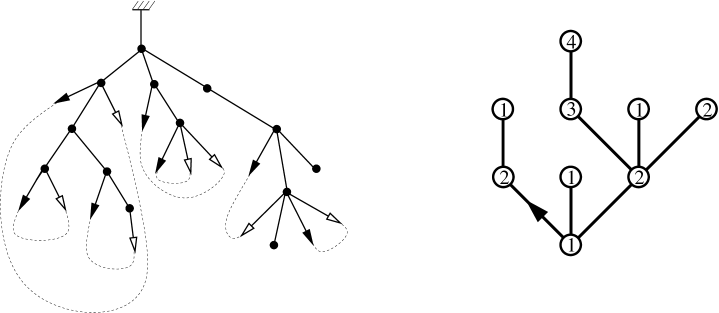
Figure 26.5: Left: a $\mathcal{S}$-tree, together with the canonical matching of black and white leaves (dashed lines between arrows). Right: a well-labeled tree.

Let us indeed define two classes of rooted trees $\mathcal{R}$ and $\mathcal{S}$ recursively as follows. A $\mathcal{R}$-tree (i.e a tree in $\mathcal{R}$) is either reduced to a “white” leaf, or it consists of a root vertex to which are attached a sequence of subtrees that can be $\mathcal{R}$-trees, $\mathcal{S}$-trees or single “black” leaves, with the condition that the number of such black leaves is equal to the number of $\mathcal{R}$-subtrees minus one. A $\mathcal{S}$-tree consists of a root vertex to which are attached a sequence of the same possible subtrees, with the condition that the number of black leaves is equal to the number of $\mathcal{R}$-subtrees. It is straightforward to check that this is a well-defined recursive construction, which translates into the equations (26.4.1) or (26.4.13) for the corresponding generating functions $R$ and $S$, provided that we attach a weight $t$ per vertex or white leaf, and a weight $v_{n}$ per vertex with $n-1$ subtrees. Figure 26.5 displays a tree in $\mathcal{S}$.

We may then wonder how such trees are related to maps. A natural idea is to “match” the black and white leaves together, creating new edges. Consider for instance a $\mathcal{S}$-tree: it has the same number of black and white leaves, and given an orientation there is a “canonical” matching procedure, see again figure 26.5. This creates a planar map out of a $\mathcal{S}$-tree, and we further observe that the vertex degrees are preserved. It is possible to show that this defines a one-to-one correspondence between $\mathcal{S}$ and the second class of maps mentioned in the remark below theorem 4, see [Bou02b] for details. We proceed similarly with $\mathcal{R}$, and then a few more steps allow to establish bijectively theorem 4. The knowledge of the matrix model solution was instrumental in “guessing” the suitable family of trees, which encompasses the one found in [Sch97] based on Tutte’s formula (26.4.22). The present construction was further extended to bipartite maps corresponding to the two-matrix model (26.3.26) [Bou02a], and maps corresponding to a chain-matrix model [Bou05].

The bijective approach has a great virtue. It was indeed realized that it is intimately connected with the “geodesic” distance in maps [Bou03]. Actually, there is another “dual” family of bijections with so-called well-labeled trees or mobiles [Cor81, Mar01, Bou04, Bou07] for which the connection is even more apparent. In the simplest instance [Cor81], a well-labeled tree is a rooted plane tree whose vertices carry a positive integer label, in such a way that labels on adjacent vertices differ by at most 1 (see again figure 26.5 for an example). It encodes bijectively a rooted quadrangulation (i.e a map whose faces have degree 4), a vertex with label $\ell$ in the tree corresponding to a vertex at distance $\ell$ from the root vertex in the quadrangulation [Mar01] (where the distance is the graph distance, i.e the minimal number of consecutive edges connecting two vertices). It is easily seen that the generating function for well-labeled trees with root label $\ell\geq 1$ satisfies

$$R_{\ell}=t+tR_{\ell}\left(R_{\ell-1}+R_{\ell}+R_{\ell+1}\right)$$ (26.5.1)

together with the boundary condition $R_{0}=0$, $t$ being a weight per edge or vertex. Through the bijection, $R_{\ell}$ yields the generating function for quadrangulations with two marked points at distance at most $\ell$, related to the so-called two-point function [Amb95]. Equation (26.5.1) is nothing but a refinement of the third relation of (26.4.15) (and we have $E_{0}^{(4)}=R_{1}/t$). Remarkably, it has an explicit solution [Bou03, section 4.1]. It furthermore looks surprisingly analogous to (yet different from) the “first string equation” (14.2.14). This still mysterious analogy is much more general, as one may refine equations (26.4.1) into discrete recurrence equations involving the distance, similar to the string equations for the one-matrix model, and having again explicit solutions [Bou03, DiF05].

The correspondence between maps and trees has sparked an active field of research between physics, combinatorics and probability theory, devoted to the study of the geometry of large random maps, see for instance [Mie09] and references therein.

References

- [Amb95] J. Ambjørn and Y. Watabiki, “Scaling in quantum gravity”, Nucl. Phys. B445 (1995) 129–144, arXiv:hep-th/9501049.
- [Ben94] E.A. Bender and E.R. Canfield, “The number of degree-restricted rooted maps on the sphere”, SIAM J. Discrete math. 7 (1994) 9–15.
- [Bou02a] M. Bousquet-Mélou and G. Schaeffer, “The degree distribution in bipartite planar maps: applications to the Ising model”, arXiv:math/0211070.
- [Bou06] M. Bousquet-Mélou and A. Jehanne, “Polynomial equations with one catalytic variable, algebraic series, and map enumeration”, Journal of Combinatorial Theory Series B 96 (2006) 623–672, arXiv:math/0504018.
- [Bou02b] J. Bouttier, P. Di Francesco and E. Guitter, “Census of planar maps: from the one-matrix model solution to a combinatorial proof”, Nucl. Phys. B645 [PM] (2002) 477–499, arXiv:cond-mat/0207682.
- [Bou03] J. Bouttier, P. Di Francesco and E. Guitter, “Geodesic Distance in Planar Graphs”, Nucl. Phys. B663 (2003) 535–567, arXiv:cond-mat/0303272.
- [Bou04] J. Bouttier, P. Di Francesco and E. Guitter, “Planar maps as labeled mobiles”, Elec. Jour. of Combinatorics 11 (2004) R69, arXiv:math/0405099.
- [Bou05] J. Bouttier, P. Di Francesco and E. Guitter, “Combinatorics of bicubic maps with hard particles”, J. Phys. A 38 (2005) 4529–4559, arXiv:math/0501344.
- [Bou07] J. Bouttier, P. Di Francesco and E. Guitter, “Blocked edges on Eulerian maps and mobiles: Application to spanning trees, hard particles and the Ising model”, J. Phys. A: Math. Theor. 40 (2007) 7411–7440, arXiv:math/0702097.
- [Bre78] É. Brézin, C. Itzykson, G. Parisi and J.-B. Zuber, “Planar diagrams”, Commun. Math. Phys. 59 (1978) 35–51.
- [Bro65] W.G. Brown, “On the existence of square roots in certain rings of power series”, Math. Ann. 158 (1965) 82–89.
- [Cor75] R. Cori, Un code pour les graphes planaires et ses applications, Société Mathématique de France, Paris 1975. With an English abstract, Astérisque 27.
- [Cor81] R. Cori and B. Vauquelin, “Planar maps are well labeled trees”, Canad. J. Math. 33 (1981) 1023–1042.
- [Cor92] R. Cori and A. Machì, “Maps, hypermaps and thier automorphisms: a survey, I, II, III” Exposition. Math. 10 (1992) 403–427, 429–447, 449–467.
- [DiF05] P. Di Francesco, “Geodesic Distance in Planar Graphs: An Integrable Approach”, Ramanujan J. 10 (2005) 153–186, arXiv:math/0506543.
- [Edm60] J.R. Edmonds, “A combinatorial representation for polyhedral surfaces”, Notices Amer. Math. Soc. 7 (1960) 646.
- [Eyn06] B. Eynard, “Formal matrix integrals and combinatorics of maps”, CRM Series Math. Phys. (to appear), arXiv:math-ph/0611087.
- [Fla08] P. Flajolet and R. Sedgewick, Analytic Combinatorics, Cambridge University Press, 2008.
- [Gim05] O. Giménez and M. Noy, “Asymptotic enumeration and limit laws of planar graphs”, J. Amer. Math. Soc. 22 (2009) 309–329, arXiv:math/0501269.
- [Hoo74] G. ’t Hooft, “A planar diagram theory for strong interactions”, Nucl. Phys. B72 (1974) 461–473
- [Kaz86] V.A. Kazakov, “Ising model on a dynamical planar random lattice: Exact solution”, Phys. Lett. A119 (1986) 140–144.
- [Kni88] V.G. Knizhnik, A.M. Polyakov and A.B. Zamolodchikov, “Fractal structure of 2D quantum gravity”, Mod. Phys. Lett. A3 (1988) 819–826.
- [Mar01] M. Marcus and G. Schaeffer, “Une bijection simple pour les cartes orientables”, manuscript (2001), available online at http://www.lix.polytechnique.fr/~schaeffe/Biblio/MaSc01.ps ; see also G. Chapuy, M. Marcus, G. Schaeffer, “A bijection for rooted maps on orientable surfaces”, SIAM Journal on Discrete Mathematics, 23(3) (2009) 1587-1611, arXiv:0712.3649.
- [Mie09] G. Miermont, “Random maps and their scaling limits”, Progress in Probability 61 (2009) 197–224.
- [Mig83] A.A. Migdal, “Loop equations and 1/N expansion”, Phys. Rep. 102 (1983) 199–290.
- [Moh01] B. Mohar and C. Thomassen, Graphs on surfaces, The John Hopkins University Press, Baltimore 2001.
- [Mul70] R.C. Mullin, E. Nemeth and P.J. Schellenberg, “The enumeration of almost cubic maps”, Proceedings of the Louisiana Conference on Combinatorics, Graph Theory and Computer Science 1 (1970) 281–295.
- [Pen88] R.C. Penner, “Perturbative series and the moduli space of Riemann surfaces”, J. Differential Geom. 27(1) (1988) 35–53.
- [Sch97] G. Schaeffer, “Bijective census and random generation of eulerian planar maps”, Elec. Jour. of Combinatorics 4 (1997) R20.
- [Tut62a] W. Tutte, “A census of planar triangulations”, Canad. J. Math. 14 (1962) 21–38.
- [Tut62b] W. Tutte, “A census of Hamiltonian polygons”, Canad. J. Math. 14 (1962) 402–417.
- [Tut62c] W. Tutte, “A census of slicings”, Canad. J. Math. 14 (1962) 708–722.
- [Tut63] W. Tutte, “A census of planar maps”, Canad. J. Math. 15 (1963) 249–271.
- [Tut68] W. Tutte, “On the enumeration of planar maps”, Bull. Amer. Math. Soc. 74 (1968) 64–74.
- [Wad81] S. R. Wadia, “Dyson-Schwinger equations approach to the large-N limit: Model systems and string representation of Yang-Mills theory”, Phys. Rev. D24 (1981) 970–-978.
- [Zvo95] A. Zvonkin, “How to Draw a Group”, Discrete Mathematics 180 (1998) 403–413.