Latent rank change detection for analysis of splice-junction microarrays with nonlinear effects

Abstract

Alternative splicing of gene transcripts greatly expands the functional capacity of the genome, and certain splice isoforms may indicate specific disease states such as cancer. Splice junction microarrays interrogate thousands of splice junctions, but data analysis is difficult and error prone because of the increased complexity compared to differential gene expression analysis. We present Rank Change Detection (RCD) as a method to identify differential splicing events based upon a straightforward probabilistic model comparing the over- or underrepresentation of two or more competing isoforms. RCD has advantages over commonly used methods because it is robust to false positive errors due to nonlinear trends in microarray measurements. Further, RCD does not depend on prior knowledge of splice isoforms, yet it takes advantage of the inherent structure of mutually exclusive junctions, and it is conceptually generalizable to other types of splicing arrays or RNA-Seq. RCD specifically identifies the biologically important cases when a splice junction becomes more or less prevalent compared to other mutually exclusive junctions. The example data is from different cell lines of glioblastoma tumors assayed with Agilent microarrays.

, , , , and

t1Corresponding author.

1 Introduction

Genomic DNA contains the sequential codes for constructing proteins that perform biochemical and structural tasks essential for life. The DNA of a gene is first transcribed into a pre-messenger RNA (pre-mRNA) transcript. The rate of transcription is referred to as gene expression and is a measure of the gene’s level of activity. The DNA fragment encoding a particular gene does not get entirely converted into mRNA. A gene is composed of sequence blocks called introns and exons. The introns are removed or spliced out of the pre-mRNA sequence, whereas the exons are retained to form the mature mRNA which is later translated into proteins. However, some exons are selectively included in the mature mRNA so that different splicing variants or isoforms result. The different splicing variants can give rise to different protein isoforms which sometimes display different structural and/or functional properties [Stryer (1995)]; see Figure 1. This is known as alternative splicing. There are several classes of alternative splicing events. For example, exon skipping occurs when an exon is selectively “skipped” or excluded in the mature mRNA. See Supplementary Figure 1 for an illustration of some common splicing events.

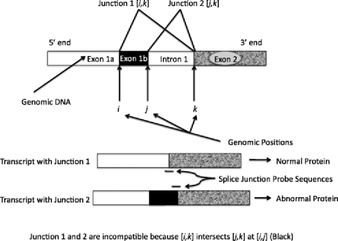
Figure 1: Schematic of splicing process, incompatible junctions and junction probes. The gene is shown at the top. The splicing process has two possibilities. First, remove exon 1b (Black) and intron 1. The fusion between exons 1a and 2 results in Junction 1. Second, only remove intron 1 while retaining exon 1b. The fusion between exons 1b and 2 results in Junction 2. The retention of exon 1b is translated into an abnormal protein, and higher fluorescence of the Junction 2 probe relative to the Junction 1 probe indicates this abnormality.

In the late 80’s and early 90’s, only a few alternative splicing events were known. Alternative splicing was considered a rare event, and its importance misunderstood. Current estimates of the number of human genes that have at least 2 splice variants range from 60 to 85% [reviewed in Cuperlovic-Culf et al. (2006)]. Different from other types of gene regulation, alternative splicing does more than simply modulate the levels of expression of affected genes. In extreme cases like the Dscam gene in Drosophila, the number of potential splice variants is equivalent to almost double the total number of genes present in the Drosophila genome [Celotto and Graveley (2001)]. Several different splicing events including exon skipping events, mutually exclusive exons and alternative $5^{\prime}$ and $3^{\prime}$ splice sites form the repertoire of alternative splicing. About 70–88% of differential splicing events affect the coding region, and the numbers of known splicing events will increase thanks to technologies such as alternative splicing arrays and RNA-Seq [Sultan et al. (2008)].

Splicing arrays contain tens or hundreds of thousands of probes that are complementary to exons or splice junctions (the fusion between exons) of the different splice isoforms of many genes. These probes bind specifically to segments within a transcript and quantify the concentrations of specific exons and splice junctions. Splicing arrays provide higher resolution measurements across the length of the transcript compared to standard expression arrays that bind to a smaller, selective portion of the transcript. See Figure 1 for the placement of splice junction probes. For a review of the different classes of alternative splicing microarrays see Moore and Silver (2008). The analysis of alternative splicing arrays is an area in need of improvement due to difficulties in estimating the relative concentrations of isoforms with or without a fully known sequence. Currently, there are several statistical methods available, but none is satisfactory because of limitations in application and inaccuracy [see Cuperlovic-Culf et al. (2006)]. The basic goal of the methods is to estimate the proportions of splice variants within a tissue and to compare these proportions between tissues. For example, we would like to estimate the relative prevalence of two isoforms in one tissue (say, a 1:2 ratio) and compare them to the relative prevalence in another tissue (say, a 2:1 ratio). If these relative prevalences are different, then we have an occurrence of differential splicing between the tissues. The analysis of alternative splicing events is a more complicated task than quantifying the overall level of expression of a gene as typically done by expression arrays. In expression analyses that compare the overall expression of a given gene in two tissues (e.g., cancer and normal), three scenarios are possible: higher expression in cancer, higher expression in normal, and equal expression. These measurements can be obtained, in principle, with one probe per gene. In alternative splicing arrays, there is a set of probes for each alternative splicing event; they normally cover splice junctions and/or the region that is alternatively spliced. A substantial percentage of human genes have two or more alternative splicing events that need to be evaluated individually. The resultant isoforms are multivariate components of the gene’s expression. Each of these isoforms itself may be up- (or down) regulated in a comparison between tissues. Further, if all of the isoforms are up- (or down) regulated, then one may additionally ask whether they occur in the same proportion in different tissues. Again, the comparisons of the relative proportions of isoforms between tissues is one of the central issues in alternative splicing analysis.

The increase in transcript information is the motivation for examining alternative splicing in cancerous tissue, but the added statistical complexity of the data requires novel and robust analytical methods. Srinivasan et al. (2005) developed the Splicing Index statistic for exon arrays. This method estimates the proportion of alternative isoforms by assuming a linear relationship between mRNA concentration and probe intensity. The analysis of splice variation (ANOSVA) proposed by Cline et al. (2005) is a similar method that uses a parametric model. ANOSVA uses a two-way analysis of variance model with an interaction where the first factor is the tissue type level (tumor, normal, etc.) and the second factor is the probe (splice junction 1, splice junction 2, etc.). In ANOSVA, the interaction between treatment effect and the probe effect corresponds to a differential splicing event (DSE). However, like the Splicing Index, ANOSVA depends on the linearity of the intensity response curve and may have a high false positive detection rate. Shai et al. (2006) presented GenASAP as another analysis method, but this potentially powerful tool has limited applicability. GenASAP uses a latent variable Bayesian model and machine learning techniques to estimate the percentage of each splice variant in a sample. Although GenASAP was designed to distinguish between only two isoforms, many genes may have multiple isoforms, and this limits the GenASAP method to a fraction of genes that only have two isoforms or to those genes that are determined by other methods to have only two prominent isoforms. Xing et al. (2008) have created normalization and analysis methods for exon array data. While their proposed normalization technique applies to splice junction arrays, the splice junction array data will likely benefit from models specifically designed for junctions. Splice junction arrays differ from exon arrays in that the probe sequences correspond to the junctions between fused exons in the final transcript. The number of possible splice junctions exceeds the number of exons because if the number of exons is $E$, the number of junctions is potentially ${E\choose 2}$, not counting partial exons, but there is a lack of knowledge about which junctions actually occur in nature. Further, unlike exons, certain splice junctions are incompatible within the same transcript based upon the topology of splicing because splicing preserves the order of the exons. For example, a transcript with a junction fusing exons 2 and 4 is incompatible with a junction fusing exons 2 and 3 because exon 3 is excluded by junctions 2–4. Our proposed method is designed to accommodate these features of junction arrays.

We present Rank Change Detection (RCD) as a method for identifying differential splicing events (DSEs) based upon a Bayesian model comparing the over or underrepresentation of two or more competing isoforms. RCD has advantages over commonly used methods as it is robust to false positive errors due to nonlinear trends in microarray measurements and it tests hypotheses of inherent biological interest. Gaidatzis et al. (2009) have recently shown that these nonlinear effects in Affymetrix exon arrays are a source of inaccuracy using current linear models, and we show that such nonlinearity is found in two color splice junction arrays as well. RCD does not depend on prior knowledge of splicing isoforms, yet it takes advantage of the inherent structure of mutually exclusive junctions. This method may easily be adapted to multiple platforms including other types of alternative splicing microarrays or RNA-Seq data.

2 Experimental design and data structure

The objective is to identify splicing differences between normal and tumor tissues or cell lines. In our experiment the normal cell line is the glial cell line known as FGG, which is compared on each array to one of four glioblastoma tumor types. This particular experimental design is called a reference design because the normal sample is used as a comparator on each array [Kerr and Churchill (2001)]. The two-color microarrays have probes that bind to splice junctions simultaneously within two samples that are labeled to fluoresce at green and red wavelengths using Cyanine-5 (Cy5) dye and Cyanine-3 (Cy3) dye, respectively. The intensity of fluorescence quantifies the amount of RNA expression. The dye orientation is balanced so that for each tumor type, the normal and tumor samples are labeled with Cy3 and Cy5, respectively, or Cy5 and Cy3, respectively, in an equal number of replicates. This is called a dye-swap design, and the experimental layout is shown in Supplemental Table 1. The log-probe intensity data for a given gene are denoted as $y_{tjrds}$ where the indices $t$, $j$, $r$, $d$ and $s$ represent tissue, junction, replicate, dye and spot respectively. Note that $t$ refers to the type of cells sampled whether from a tissue or a cell line or culture, but we will refer to $t$ as tissue without loss of generality. We found that there was little to no dye bias so we drop this distinction (index $d$) for convenience. The spot or probe effect induces correlation between the red and the green channels that are measured for each probe. The junction $j$ is defined by the location (in DNA base pairs or bp) from the transcription start site (or another reference site) of the $5^{\prime}$ and the $3^{\prime}$ sites ($j_{5}$ and $j_{3}$) that define the interval $[j_{5},j_{3}]$ of the excised segment of the transcript. Two junctions $j$ and $j^{\prime}$ are mutually incompatible if $[j_{5},j_{3}]\cap[j^{\prime}_{5},j^{\prime}_{3}]\neq\varnothing$. The nonempty intersection indicates that one junction excises a component of the other, thus making mutually exclusive within the same transcript; see Figure 1. The set of all junctions incompatible with junction $j$ is denoted as $O_{j}$. This implies that the junction $j$ is in the set of incompatible junctions $O_{j}$ ($j\in O_{j}$). There are possibly more incompatible junctions in the set $O_{j}$ if one had knowledge of biologically plausible transcripts and their corresponding junctions. Our method of defining incompatible sets has the advantage that it does not require that the full transcript sequences are known. The specification of these sets is critical because this defines the set of junctions whose proportions are being compared. One typically compares the relative prevalence $p_{tj^{\prime}}$ of the junctions $j^{\prime}\in O_{j}$ for each tissue $t_{1},t_{2}$ where $\sum_{j^{\prime}\in O_{j}}p_{tj^{\prime}}=1$, and the null hypothesis for a differential splicing event (DSE) is $p_{t_{1}j^{\prime}}=p_{t_{2}j^{\prime}}$ for $j^{\prime}\in O_{j}$.

3 Rank change detection method

The model of Cline et al. (2005) is an ANOVA model described by $E[y_{tjr}]=\mu_{tj}=\mu_{0}+\alpha_{t}+\beta_{j}+\gamma_{t\times j}$ and $\alpha$, $\beta$ and $\gamma$ are the effects of tissue, junction and the interaction between the tissue and junction. The rejection of the test of $\gamma_{t\times j}=0$ implies a differential splicing event. That is, the $\gamma_{t\times j}$ represents the relative increase or decrease in the junction $j$ prevalence in tissue $t$. However, the model becomes invalid in the presence of nonlinearity. For example, if there is not a DSE and there are two incompatible junctions ($A$ and $B$), then we denote the mean intensities of the probes by $\mu_{tj,}$ say, $\mu_{NA}$, $\mu_{NB}$, $\mu_{CA}$ and $\mu_{CB}$ where $N$ and $C$ are the normal and cancer tissue indices. According to the ANOSVA model, $\mu_{tj}=\mu_{0}+\alpha_{t}+\beta_{j}+\gamma_{t\times j}$, so that if $\gamma_{t\times j}=0$, then $\mu_{CA}-\mu_{NA}=\mu_{CB}-\mu_{NB}$. Equivalently, if there is no DSE, then the difference between junction probe mean intensities should be equal. Substantial nonlinearity results in an extremely high false positive rate due to the phenomenon in Figure 2A. For example, we examine our data for the VIM gene shown in Figure 3. On the vertical axis is the estimate of the mean junction differences ($\hat{\mu}_{Cj}-\hat{\mu}_{Nj}$), and on the horizontal axis is the estimate of the mean junction intensity $\frac{1}{2}(\hat{\mu}_{Cj}+\hat{\mu}_{Nj})$. Clearly, the difference $\hat{\mu}_{Cj}-\hat{\mu}_{Nj}$ is not equal for all junctions with the high and low intensity junctions having differences closer to 0. This dependence on intensity is consistent with nonlinear response as in Figure 2A. The ANOSVA test for $\gamma_{t\times j}=0$ results in a $p$-value $<10^{-19}$, which would likely yield a false positive result because nonlinear response to differential expression is confounded with the hypotheses about junction by tissue interactions.

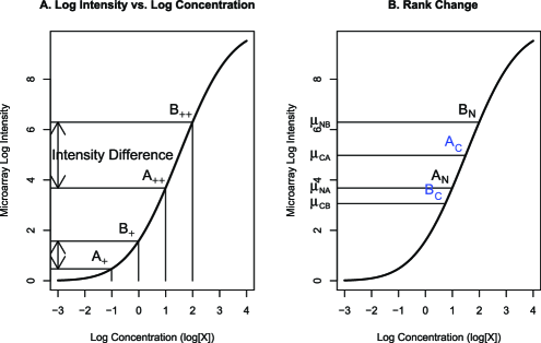
Figure 2: (A) Example of sigmoidal response of microarray Intensity: Two incompatible isoforms A and B present in 1:2 a ratio at high ($++$) and low ($+$) levels of overall gene expression. Notice that the intensity difference between the two isoforms is narrowed considerably in lower concentration despite the constant concentration ratio of 2:1. Models assuming linearity could falsely estimate that the ratio of isoforms had narrowed from 2:1 to closer to 1:1. (B) Rank Changes of isoform intensity are invariant under monotonic transformation. There are two incompatible isoforms A and B present in normal (N), cancer (C). Isoform A is more prevalent in cancer, while isoform B is more prevalent in normal. The proposed method identifies such changes in prevalence rankings of isoforms. The mean intensities are shown on the vertical axis as $\mu_{tj}$.

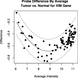
Figure 3: Difference vs Average plot for splice junctions of theVIM gene. Each point is the average value of a specific junction. The horizontal axis is the estimate of the mean junction intensity $\frac{1}{2}(\hat{\mu}_{Cj}+\hat{\mu}_{Nj})$, and the vertical axis is the estimate of the mean junction differences ($\hat{\mu}_{Cj}-\hat{\mu}_{Nj}$). Note the substantial nonlinear effect apparent in the parabolic trend. This invalidates algorithms based upon linearity such as ANSOVA likely resulting in false positives.

We propose a model for rank change that tests the hypothesis that a junction has the same rank in relative proportion in one tissue compared to another, as measured by probe intensity. We define the rank of $p_{tj}$ as $R(p_{tj})=\sum_{j^{\prime}\in O_{j}}I[p_{tj^{\prime}}\leq p_{tj}]$ where $I[\cdot]$ is the indicator function. Instead of the null hypothesis that proportions themselves are equal, $p_{t_{1}j^{\prime}}=p_{t_{2}j^{\prime}}$ for $j^{\prime}\in O_{j}$, we will test that the ranks of the $p_{tj}$ are equal, $R(p_{t_{1}j^{\prime}})=R(p_{t_{2}j^{\prime}})$ for $j^{\prime}\in O_{j}$, by making the reasonable assumption that the ranks in mean junctions intensities $\mu_{tj}$ approximate the ranks of the junction proportions $p_{tj}$. A shift in rank represents a decrease or increase in the prevalence of the isoform as shown in Figure 2B. The justification for assessing ranks is that ranks are preserved under monotonic transformation due to nonlinear response, whereas differences in intensity (i.e., $\gamma_{C\times j}=\hat{\mu}_{Cj}-\hat{\mu}_{Nj}$) are not. We propose the following random effects implementation of the ANOSVA model for two color arrays:

$$y_{tjrs}=\mu_{tj}+\nu_{tjrs}+\varepsilon_{tjrs},$$ (1)

where the $\mu_{tj}$ are the means of the $j$th junction in $t$th tissue and $\varepsilon_{tjr}$ is an independent Gaussian noise error term. The term $\nu_{tjrs}$ is a Gaussian random effect corresponding to a probe on an array, and this random effect is two-dimensional corresponding to the red and green dyes. The main idea of detecting rank change comes from the following example. If there is not a DSE and there are only two junctions ($A$ and $B$), then the ranks of the mean intensities ($\mu_{tj^{\prime}},j^{\prime}\in O_{j}$) are preserved. In other words, $\mu_{NA}<\mu_{NB}$ implies that $\mu_{CA}<\mu_{CB}$ where $N$ and $C$ are the normal and cancer tissue indices. This is equivalent to saying junction $B$ is more prevalent than junction $A$ in both tissues, assuming that intensities of the two junction probes roughly reflect their relative concentrations. If the ranks of the junction prevalences change as in Figure 2, then there is a DSE. For an arbitrary number of isoforms, no DSE implies that the ranks of the $\mu_{tj}$ are preserved across tissues. We do not directly observe the ranks of the latent means $\mu_{tj}$ as there is variability in measurement, but we can estimate the latent ranks of the means from the posterior distribution. Let the rank of the mean intensity $\mu_{tj}$ of junction $j$ within a tissue $t$ be defined as $R(\mu_{tj})=\sum_{j^{\prime}\in O_{j}}I[\mu_{tj^{\prime}}\leq\mu_{tj}]$. Our null hypothesis for a DSE between tissues $t_{1}$ and $t_{2}$ would be that

$$R(\mu_{t_{1}j})=R(\mu_{t_{2}j}).$$

That is, the rank of the average intensity of junction $j$ relative to other incompatible junctions $j^{\prime}\in O_{j}$ is preserved across tissues. Since there are 40,000 models corresponding to each junction on the chip, we will estimate the posterior distributions using approximations to accelerate model fitting. We can approximate the posterior distributions of $\mu_{tj}$ by the maximum likelihood theory point and variance estimates ($\hat{\mu}_{tj}$ and $\hat{\Sigma}_{\mu}$). We estimate and compare the posterior distributions of $R(\mu_{t_{1}j})$ and $R(\mu_{t_{2}j})$ with Monte-Carlo integration of the posterior distribution $p([\mu_{t1},\ldots,\mu_{tJ}]|\mathrm{Data})$ where $J=$ size of $O_{j}$. The posterior distributions of $R(\mu_{tj})$ are approximated by computing $\sum_{j^{\prime}\in O_{j}}I[\mu_{tj^{\prime}}\leq\mu_{tj}]$ from samples of $[\mu_{t1},\ldots,\mu_{tJ}]$ drawn from the multivariate Gaussian with mean $[\hat{\mu}_{t1},\ldots,\hat{\mu}_{tJ}]$ and variance $\hat{\Sigma}_{\mu}$. We define the posterior probability of a rank increasing ($U$) or decreasing ($D$) DSE as $\operatorname{Pr}(R(\mu_{t_{1}j})>R(\mu_{t_{2}j}))=D_{t_{1}t_{2}j}$ and $\operatorname{Pr}(R(\mu_{t_{1}j})<R(\mu_{t_{2}j}))={U}_{t_{1}t_{2}j}$ and estimate these with the Monte-Carlo sample proportions satisfying these events. If $\max(U_{t_{1}t_{2}j},D_{t_{1}t_{2}j})>\kappa$ where $\kappa$ is a cutoff (say 0.9), then we declare junction $j$ differentially spliced between tissues $t_{1}$ and $t_{2}$.

We use the term latent ranks because it is important to distinguish the proposed method of ranking the posterior means from the typical use of rank statistics computed directly from the observed values. For example, Tan et al. (2005) use rank reversals for microarray classification in a method called Top Scoring Pairs, and they compute the ranks of the raw microarray intensities and characterize the variability of the ranks based upon the observed frequencies of orderings. Given that microarray experiments have substantial measurement error as well as potentially large effect sizes, we need to maximize the accuracy and carefully quantify variability in rank estimates. When the sample sizes are small as is often the case in differential splicing experiments, using the ranks of the posterior means may have advantages over using the frequencies of the orderings. Figure 4 shows two scenarios of how the ranks of posterior means lead to different results than using the observed ranks. The axes are the log expression levels of 2 junctions, and the $95\%$ highest posterior density (HPD) regions of the posterior means are outlined. Case 1 demonstrates that one may estimate the posterior rank of the mean of Junction 2 to be higher than Junction 1 with $95\%$ confidence given only two observations if Junction 2 is much greater than 1 relative to the error variance. However, if one considered relative frequencies of the ranks of two randomly ordered pairs, then the pattern would occur $25\%$ of the time. In case 2, there are four observations, and 3 out of 4 show Junction 2 having higher rank than 1. Because the posterior density has a small variance, the posterior mean of Junction 2 has a $95\%$ probability of being higher than Junction 1 even though $25\%$ of the observations show this not to be the case. RCD maintains high power in low sample size compared to other ranking methods because it does not use the raw ranks as it takes into account the magnitude of differences relative to the variances and not just the observed ordering. Therefore, using the posterior ranks of means gives different results from using the raw ranks, and this is appropriate for detecting associations of relative junction prevalence with biological condition in experiments with small sample sizes. However, using the frequency of observed ranks as in Tan et al. (2005) is more appropriate for discriminating biological states for the purposes of classification with relatively large sample sizes.

The accuracy of the posterior relies upon distributional assumptions and the reasonableness of the prior. The distributional assumption of the normality of residuals is an accepted approximation for microarrays [Cline et al. (2005); Kerr and Churchill (2001)], and we found this is reasonable for our data. We chose a noninformative prior based upon the MLE approximation, but one may tune the influence of the prior by altering the threshold $\kappa$ to be more or less conservative. It is conceivable to avoid the use of priors by constructing a frequentist test for latent rank, but this could be relatively cumbersome given the difficulty of maximum likelihood estimation on the discrete rank space.

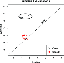
Figure 4: A hypothetical experiment demonstrating that the posterior ranks of the means provide more evidence compared to the ranks of the raw observations. The $95\%$ HPDs for the posterior means are drawn as ellipses. In both cases, the prevalence of Junction 2 is greater than Junction 1. In case 1, there are only 2 observations, but the posterior distribution strongly favors higher rank for Junction 1. However, this frequency of observed ranks would randomly occur $25\%$ of the time. In case 2, there is $>95\%$ posterior probability that Junction 2 has higher mean than Junction 1, even though the observed relative frequency that Junction 2 is greater than Junction 1 is only $75\%$. The accuracy of the evidence from the posterior depends upon parametric assumptions.

The model identifies the event that the prevalence of one junction surpasses or becomes less than another junction in different tissues. This model detects a shift in intensity ratios between junctions such as 1:2 changing to 2:1, but the model does not detect changes in ratios such as 3:5 changes to 4:5. This way, the rank change model tests qualitative changes in prevalence such as when isoforms go from dominant (highest rank) to nondominant (lesser rank) rather than detecting merely quantitative changes in junction prevalence. We suggest that such qualitative changes have more biological impact and are worth specific detection algorithms. The RCD method is implemented in the R programming language, and is available at http://sites.google.com/site/gbiostats/.

4 Simulation study

We performed a simulation to directly compare the performance of the RCD method to ANOSVA in terms of the false positive rate. We anticipated that ANOSVA would perform well in the absence of nonlinearity, but in the presence of nonlinearity, it would have an unacceptably high false positive rate. We simulated data under 4 different scenarios: 2 incompatible isoforms and linear response, 2 isoforms and nonlinear response, 3 incompatible isoforms and linear response, and 3 incompatible isoforms and nonlinear response. We used the previously discussed ANOSVA model for simulation $E[y_{tjr}]=\mu_{tj}=\alpha_{t}+\beta_{j}+\gamma_{t\times j}$. In each case, we had 2 tissue types and 12 two color arrays in a balanced, dye-swap design. The tumor tissue differential expression effect ($\alpha_{t}$) was simulated to consist of a log fold-change using a Gaussian distribution of mean 0, standard deviation 1, and the normal tissue level was drawn from the empirical distributions of the means of the normal cells in our data set. The relative prevalences of the incompatible junctions ($\exp(\beta_{j})$) were simulated from different Dirichlet distributions with parameters (1,1) for 2 junctions or (1,1,1) for 3 junctions. Because we are estimating the false positive rates, the simulation examines scenarios such that there are no differential splicing events ($\gamma_{t\times j}=0$). The random error was an empirical distribution of the residuals of the reference channel with mean 0 and standard deviation of $0.22$, and no spot specific effects were simulated, as these effects were observed to be relatively small in the data. The nonlinear effect was simulated by transforming $E[y_{tjr}]$ with a linear transformation of a logistic function that approximates the dynamic range of the array $P(x)=w/(1+\exp(-(x-\mu^{*})/\sigma^{*}))+\delta_{\mathrm{min}}$ where $w=9.2$ is the width of the observed dynamic range on the log scale; $\delta_{\mathrm{min}}=6.3$ is the minimum of the dynamic range; $\mu^{*}=10.9$ is the midpoint between the minimum and maximum of the dynamic range; and $\sigma^{*}$ is selected so that $P(x)$ has slope${}=1$ when $x=\mu^{*}$. The estimate of the false positive rate was based upon a $p$-value cutoff of 0.05 for the ANOSVA model ($\gamma_{t\times j}=0$), and a cutoff of posterior probability of unequal ranks of $\kappa=0.9$ for the rank change model. We obtained the false positive rates for 1000 simulations as shown in Table 1.

The false positive rate of ANOSVA is close to the nominal 0.05 value under the linear scenarios, albeit somewhat inflated due to slight violations of parametric assumptions, but ANOSVA has a substantially inflated false positive rate of 3–4 times higher than the nominal value under the nonlinear scenarios. In contrast, the cutoff of 0.9 probability of differential splicing has a tolerably low false positive rate. The simulation suggests that the nominal $p$-values obtained for differential splicing detection could lead to an unacceptably high rate of false positive calls in the presence of nonlinearity. In general, we found that estimation of larger numbers of mutually incompatible junctions resulted in more false positives for both models. For this reason, we recommend that the maximum size of $O_{j}$ considered be less than 10 or to adjust the posterior probability cutoff for larger $O_{j}$.

Table 1: False positve rate for RCD model and conventional ANOSVA model

	Model
Scenario	ANOSVA	RCD
2 junction linear	0.063	0.000
2 junction nonlinear	0.165	0.008
3 junction linear	0.057	0.001
3 junction nonlinear	0.194	0.010

We also performed a power analysis to demonstrate that the power loss due to the use of ranks is not too great compared to ANOSVA. We considered power in both the linear and the nonlinear cases for two opposing junctions, and we simulated random error and tissue effects based upon empirical values as previously described. The interaction between tissue and junction was selected to be rank reversals of two opposing junctions such that a ratio of prevalence of $x\dvtx y$ in one tissue is reversed to $y\dvtx x$ in the other tissue. Without loss of generality, if $x=1$, then the effect size of the interaction log scale would be $2\log_{2}(y)$. We varied the effect size from $\log_{2}(1)$ to $2\log_{2}(8)$ for the nonlinear case and from $\log_{2}(1)$ to $2\log_{2}(1.5)$ in the linear case, and varied the sample size from $n=4$ to $12$. When the interaction effect size is $0=\log_{2}(1)$, the junction effect is equal in both tissues and chosen at random from the range of $\log_{2}(1.5)$ to $\log_{2}(8)$ for the nonlinear case and from $\log_{2}(1.05)$ to $\log_{2}(1.5)$ in the linear case. The results of $1000$ simulations per scenario are shown in Supplementary Figure 2. In the nonlinear case, ANOSVA has Type I error rate of $0.212$ and $0.308$ for sample sizes of 4 and 12, respectively, compared to $0.004$ and $0.000$ for the RCD model. The power comparison in the nonlinear case favors ANOSVA by approximately $10\%$, although this is balanced by an increase in the Type I error of more than 10-fold. In the linear scenario, the relative power of ANOSVA vs. RCD is similar to the nonlinear scenario while the sensitivity of both methods to detect DSE is increased. In the power comparison, there are two issues that need to be emphasized. First, the RCD model detects only cases when there is a qualitative difference in rank so that quantitative changes in prevalence such as 1:2 to 1:3 cannot be reliably detected. Second, the posterior probabilities given by RCD and the $p$-values of ANOSVA have different meanings, and this complicates direct comparisons.

5 Application to glioblastoma data

We studied one normal brain cell line (FGG) and four glioma lines (U87MG, U118MG, T98G and A172). The arrays used in our analysis were designed by JIVAN Biologicals (San Francisco, CA) and manufactured by Agilent (Santa Clara, CA). They contain 2145 genes identified to be related to cancer by literature search. There were 38,425 splice junctions or potential alternative splicing events represented on the arrays as probes of length 35–40 bp. The probe sequences were based upon build hg17 and can be downloaded with the raw and normalized data from the Gene Expression Omnibus (GPL10127 and GSE20723). 200 ng of each RNA sample were labeled with Cy3/Cy5 dye using Agilent Low RNA Input Linear Amplification kit as per manufacturers protocols. After amplification, 750 ng each of Cy3 and Cy5 labeled RNA were combined and hybridized to microarrays. A two color microarray based gene expression analysis protocol (Agilent) was used. The normal FGG line was used as a reference for all arrays in a dye-swap design with the 4 glioma lines being labeled Cy3 and Cy5 two times each for a total of 16 arrays. See Supplemental Table 1 for a layout of the experimental design. Microarrays were scanned using the Agilent Microarray Scanner G2565AA and extracted using Agilent feature Extraction Software version 9.1. Array data preprocessing and normalization were performed using the SpliceFold software JIVAN Biologicals (San Francisco, CA).

The size of the sets of incompatible junctions considered ranged from 2 to 10. The percentages of sets with 2, 3, 4 and 5 junctions were 31%, 19%, 11% and 8%, respectively. We examined the incompatible sets corresponding to each junction. The RCD model fit indicates that hundreds of junctions have posterior probability for rank change of $>0.9$; see Table 2A. Note that some events counted may be interrelated, as some sets of incompatible junctions have nonnull intersections. A full list of the significant genes and junctions are downloadable from the url. We also compared the results with the ANOSVA method shown in Table 2B. Here, a junction is called differentially spliced if the false discovery rate (FDR) estimated by the qvalue is less than 0.1 [Storey and Tibshirani (2003)]. The qvalue criterion is inherently more liberal than the posterior probability criterion, but this difference is modest. Table 2C demonstrates the overlapping significant junctions satisfying both criteria for the RCD and the ANOSVA models. Note that most of the junctions identified as significant according to the rank change model are declared significant according to ANOSVA model. The number of junctions identified by ANOSVA is much higher, although, we argue, that the results are heavily confounded with the substantial differential expression within the experiment. To demonstrate the confounding between differential expression and the differential splicing events estimated by ANOSVA, we tested the hypothesis that the junctions that were differentially expressed were more likely to be declared a DSE. By differentially expressed, we mean that the average expression in one cell line is higher than the other for a given set of junctions. Figure 5 shows evidence for differential splicing events estimated by ANOSVA and the RCD model and their relationship to the estimated differential expression. The evidence for a DSE for the ANOSVA model is quantified by the local false discovery rate (lFDR) [Pounds and Cheng (2006)]. In Figure 5A, the ANOSVA model estimate of local false discovery rate for differential splicing (Posterior Probability of No DSE) has a strong dependency on the log fold change estimate for differential expression. This indicates the higher fold change estimates for differential expression imply higher posterior probability of differential splicing. This is consistent with the idea that the nonlinear effects within the microarray confound the hypotheses about splicing and differential expression, and that the estimates of differential splicing are biased and substantially overestimated. In Figure 5B, the RCD model estimate for differential splicing probability has little dependency on overall changes in expression. This is consistent with the robustness of the rank change model to bias due to change in expression level.

Table 2: Number of alternative splicing events between cell types for RCD and ANOSVA models

	Cell type	FGG	A172	T98G	U118
A. RCD	A172	0364
	T98G	0344	00.365
	U118	0389	00.348	0399
	U87	0333	00.334	0311	0264
B. ANOSVA	A172	6058
	T98G	7610	11,106
	U118	7771	0.8695	8890
	U87	6590	0.8319	7546	5048
C. RCD & ANOSVA	A172	0267
	T98G	0286	00.346
	U118	0351	00.316	0367
	U87	0301	00.282	0274	0213

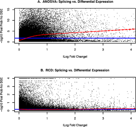
Figure 5: Splicing Probability vs differential expression Log Fold Change. (A) The ANOSVA model estimate of local false discovery rate for differential splicing ($-\log_{10}$ Posterior Probability of No DSE) has a strong dependency on differential expression fold change ($|\log\mbox{Fold Change}|$). A spline curve is shown in red, and the mean $-\log_{10}$ lFDR of differential splicing is in blue. This indicates that the higher fold change for differential expression implies higher probability of differential splicing. The nonlinear effects within the microarray confound the hypotheses about splicing and differential expression. (B) The RCD model estimate for differential splicing probability has little dependency on overall changes in expression. A spline curve is shown in red, and the mean $-\log_{10}$ posterior probability of no differential splicing is in blue.

We also examined whether the genes with splicing events reported in the literature for glioblastoma had greater posterior probability for splicing under the ANOSVA and the RCD models. Cheung et al. (2008) reported such genes from multiple studies, including 8 that were assessed by our arrays: CALD1, CASP2, FGFR1, NF1, RAB3A, ST18, TNC and TPD52L2. For all comparisons between cell types, we computed the enrichment ratio which we define as the proportion of significant DSEs in the previously reported genes relative to proportion of significant DSEs in all other genes at various cutoffs. The cutoffs we used for the RCD model were posterior probabilities for rank change greater than 90%, 99%, 99.9% and 99.99%, and the cutoffs for ANOSVA were lFDR values of less than $10^{-1,-2,-3,\ldots,-15}$. The results are in Supplemental Tables 2 and 3. The enrichment ratio peaked at 3.17 for ANOSVA when the cutoff was $10^{-14}$, giving 36 significant DSEs in the known genes. The enrichment ratio plateaued at 13 for RCD when the cutoff was 99.99%, giving 18 significant DSEs in the same genes. However, at the corresponding cutoffs in RCD and ANOSVA resulting in 36 significant DSEs in the known genes, the RCD enrichment ratio was 6.7 compared to 3.17 for ANOSVA. This implies that the RCD method found that the known genes were substantially more enriched for DSEs than the ANOSVA method for equally conservative cutoffs. We repeated the above enrichment score estimation with randomly selected sets of 8 genes, and found that $<1\%$ of these sets give a DSE enrichment score greater than the known genes.

6 Discussion

We presented a model for the detection of differential splicing events in the presence of substantial nonlinear effects of the microarray intensity response. This model is robust to the violations of the assumption of linearity and is designed to detect features of alternative splicing that are invariant under monotonic transformation. One difficulty with the model is that differential splicing may occur without exhibiting the invariant feature of rank change. Although these features are likely present in the most dramatic and biologically important differential splicing events, the proposed model may have lower power to detect more subtle shifts in the proportions of isoforms expressed in different tissues. We choose to trade sensitivity for specificity in the current setting as the false positive rate (though not knowable) is potentially quite high for other methods. This method may be used with either one- or two-color splice junction array technology and can be applied to data with or without nonlinear effects to identify qualitative changes in junction prevalence. It may be argued that filtering out either very low or very high measurements from downstream analysis would reduce the degree of nonlinearity in the data. However, the selection of a cutoff would be difficult and error prone. Furthermore, very high and very low intensities can be informative so that the removal of meaningful measurements degrades the signal in the data.

There are several opportunities to extend the proposed model. We estimated the posterior distribution based upon the MLE, and this has the effect of selecting noninformative priors. Noninformative priors imply that there is an equal probability of there being an alternative splicing event or not, but the accuracy of the method could be improved if one utilized data on the prior probability of particular alternative splicing events. The hypothesis of rank change can be extended to any model for which there are posterior distributions of parameters related to the ranks of relative isoform prevalence. First, we may explicitly model the sigmoidal response of the microarray intensity with some appropriate parametric link function $g(\cdot)$ so that we have $g(E[y_{tjr}])=\mu_{0}+\alpha_{t}+\beta_{j}+\gamma_{t\times j}$. This would likely add to the computational challenge of fitting the model, but it would improve sensitivity to detect DSEs. If we next consider $g(\cdot)$ as a link function in a log-linear count model, we may model splice junction counts from RNA-seq data instead of microarray intensity. Second, we had assumed that the error terms $\varepsilon_{tjr}$ were independent of one another, although it is likely that the incompatible isoforms have errors that are negatively correlated, and these correlations of the residuals can be modeled using a compound symmetric structure. Third, we may extend the model to include knowledge of the transcripts by adding a latent variable for each known isoform such that

$$y_{tjr}=\sum_{h}\beta_{j}z_{ht}\delta_{hj}+\nu_{tjr}+\varepsilon_{tjr},$$ (2)

where $\beta_{j}$ is the effect of junction $j$, $z_{ht}$ is the latent variable proportional to the amount of isoform $h$ within the tissue $t$, and $\delta_{hj}$ is the indicator variable for whether or not junction $t$ is within junction $h$. This extension could incorporate exon probes as well. The latent variable $z_{ht}$ would be an indication of the prevalence of the isoform, and estimating the ranks and differences in $z_{ht}$ would help to identify differential splicing events by pooling information across junctions and exons within a complete isoform.

References

- Celotto and Graveley (2001) {barticle}[author] \bauthor\bsnmCelotto, \bfnmAM\binitsA. and \bauthor\bsnmGraveley, \bfnmBR\binitsB. (\byear2001). \btitleAlternative splicing of the Drosophila Dscam pre-mRNA is both temporally and spatially regulated. \bjournalGenetics \bvolume159 \bpages599–608. \endbibitem
- Cheung et al. (2008) {barticle}[author] \bauthor\bsnmCheung, \bfnmHannah C.\binitsH. C., \bauthor\bsnmBaggerly, \bfnmKeith A.\binitsK. A., \bauthor\bsnmTsavachidis, \bfnmSpiridon\binitsS., \bauthor\bsnmBachinski, \bfnmLinda L.\binitsL. L., \bauthor\bsnmNeubauer, \bfnmValerie L.\binitsV. L., \bauthor\bsnmNixon, \bfnmTamara J.\binitsT. J., \bauthor\bsnmAldape, \bfnmKenneth D.\binitsK. D., \bauthor\bsnmCote, \bfnmGilbert J.\binitsG. J. and \bauthor\bsnmKrahe, \bfnmRalf\binitsR. (\byear2008). \btitleGlobal analysis of aberrant pre-mRNA splicing in glioblastoma using exon expression arrays. \bjournalBMC Genomics \bvolume9, article 216. \endbibitem
- Cline et al. (2005) {barticle}[author] \bauthor\bsnmCline, \bfnmMS\binitsM., \bauthor\bsnmBlume, \bfnmJ\binitsJ., \bauthor\bsnmCawley, \bfnmS\binitsS., \bauthor\bsnmClark, \bfnmTA\binitsT., \bauthor\bsnmHu, \bfnmJS\binitsJ., \bauthor\bsnmLu, \bfnmG\binitsG., \bauthor\bsnmSalomonis, \bfnmN\binitsN., \bauthor\bsnmWang, \bfnmH\binitsH. and \bauthor\bsnmWilliams, \bfnmA\binitsA. (\byear2005). \btitleANOSVA: A statistical method for detecting splice variation from expression data. \bjournalBioinformatics \bvolume21 \bpagesI107–I115. \endbibitem
- Cuperlovic-Culf et al. (2006) {barticle}[author] \bauthor\bsnmCuperlovic-Culf, \bfnmMiroslava\binitsM., \bauthor\bsnmBelacel, \bfnmNabil\binitsN., \bauthor\bsnmCulf, \bfnmAdrian S.\binitsA. S. and \bauthor\bsnmOuellette, \bfnmRodney J.\binitsR. J. (\byear2006). \btitleMicroarray analysis of alternative splicing. \bjournalOmics-A Journal of Integrative Biology \bvolume10 \bpages344–357. \endbibitem
- Gaidatzis et al. (2009) {barticle}[author] \bauthor\bsnmGaidatzis, \bfnmD\binitsD., \bauthor\bsnmJacobeit, \bfnmK\binitsK., \bauthor\bsnmOakeley, \bfnmEJ\binitsE. and \bauthor\bsnmStadler, \bfnmMB\binitsM. (\byear2009). \btitleOverestimation of alternative splicing caused by variable probe characteristics in exon arrays. \bjournalNucleic Acids Res. \bvolume37 \bpagese107. \endbibitem
- Kerr and Churchill (2001) {barticle}[author] \bauthor\bsnmKerr, \bfnmM. K.\binitsM. K. and \bauthor\bsnmChurchill, \bfnmG. A.\binitsG. A. (\byear2001). \btitleExperimental design for gene expression microarrays. \bjournalBiostatistics \bvolume2 \bpages183–201. \endbibitem
- Moore and Silver (2008) {barticle}[author] \bauthor\bsnmMoore, \bfnmMichael J.\binitsM. J. and \bauthor\bsnmSilver, \bfnmPamela A.\binitsP. A. (\byear2008). \btitleGlobal analysis of mRNA splicing. \bjournalRNA-A Publication of the RNA Society \bvolume14 \bpages197–203. \endbibitem
- Pounds and Cheng (2006) {barticle}[author] \bauthor\bsnmPounds, \bfnmStan\binitsS. and \bauthor\bsnmCheng, \bfnmCheng\binitsC. (\byear2006). \btitleRobust estimation of the false discovery rate. \bjournalBioinformatics \bvolume22 \bpages1979–1987. \endbibitem
- Shai et al. (2006) {barticle}[author] \bauthor\bsnmShai, \bfnmO\binitsO., \bauthor\bsnmMorris, \bfnmQD\binitsQ., \bauthor\bsnmBlencowe, \bfnmBJ\binitsB. and \bauthor\bsnmFrey, \bfnmBJ\binitsB. (\byear2006). \btitleInferring global levels of alternative splicing isoforms using a generative model of microarray data. \bjournalBioinformatics \bvolume22 \bpages606–613. \endbibitem
- Srinivasan et al. (2005) {barticle}[author] \bauthor\bsnmSrinivasan, \bfnmK\binitsK., \bauthor\bsnmShiue, \bfnmL\binitsL., \bauthor\bsnmHayes, \bfnmJD\binitsJ., \bauthor\bsnmCenters, \bfnmR\binitsR., \bauthor\bsnmFitzwater, \bfnmS\binitsS., \bauthor\bsnmLoewen, \bfnmR\binitsR., \bauthor\bsnmEdmondson, \bfnmLR\binitsL., \bauthor\bsnmBryant, \bfnmJ\binitsJ., \bauthor\bsnmSmith, \bfnmM\binitsM., \bauthor\bsnmRommelfanger, \bfnmC\binitsC., \bauthor\bsnmWelch, \bfnmV\binitsV., \bauthor\bsnmClark, \bfnmTA\binitsT., \bauthor\bsnmSugnet, \bfnmCW\binitsC., \bauthor\bsnmHowe, \bfnmKJ\binitsK., \bauthor\bsnmMandel-Gutfreund, \bfnmY\binitsY. and \bauthor\bsnmAres, \bfnmM\binitsM. (\byear2005). \btitleDetection and measurement of alternative splicing using splicing-sensitive microarrays. \bjournalMethods \bvolume37 \bpages345–359. \endbibitem
- Storey and Tibshirani (2003) {barticle}[author] \bauthor\bsnmStorey, \bfnmJ. D.\binitsJ. D. and \bauthor\bsnmTibshirani, \bfnmR.\binitsR. (\byear2003). \btitleStatistical significance for genome-wide studies. \bjournalProc. Natl. Acad. Sci. USA \bvolume100 \bpages9440–9445. \MR1994856 \endbibitem
- Stryer (1995) {bbook}[author] \bauthor\bsnmStryer, \bfnmL.\binitsL. (\byear1995). \btitleBiochemistry. \bpublisherFreeman, \baddressNew York. \endbibitem
- Sultan et al. (2008) {barticle}[author] \bauthor\bsnmSultan, \bfnmMarc\binitsM., \bauthor\bsnmSchulz, \bfnmMarcel H.\binitsM. H., \bauthor\bsnmRichard, \bfnmHugues\binitsH., \bauthor\bsnmMagen, \bfnmAlon\binitsA., \bauthor\bsnmKlingenhoff, \bfnmAndreas\binitsA., \bauthor\bsnmScherf, \bfnmMatthias\binitsM., \bauthor\bsnmSeifert, \bfnmMartin\binitsM., \bauthor\bsnmBorodina, \bfnmTatjana\binitsT., \bauthor\bsnmSoldatov, \bfnmAleksey\binitsA., \bauthor\bsnmParkhomchuk, \bfnmDmitri\binitsD., \bauthor\bsnmSchmidt, \bfnmDominic\binitsD., \bauthor\bsnmO’Keeffe, \bfnmSean\binitsS., \bauthor\bsnmHaas, \bfnmStefan\binitsS., \bauthor\bsnmVingron, \bfnmMartin\binitsM., \bauthor\bsnmLehrach, \bfnmHans\binitsH. and \bauthor\bsnmYaspo, \bfnmMarie-Laure\binitsM.-L. (\byear2008). \btitleA global view of gene activity and alternative splicing by deep sequencing of the human transcriptome. \bjournalScience \bvolume321 \bpages956–960. \endbibitem
- Tan et al. (2005) {barticle}[author] \bauthor\bsnmTan, \bfnmAC\binitsA., \bauthor\bsnmNaiman, \bfnmDQ\binitsD., \bauthor\bsnmXu, \bfnmL\binitsL., \bauthor\bsnmWinslow, \bfnmRL\binitsR. and \bauthor\bsnmGeman, \bfnmD\binitsD. (\byear2005). \btitleSimple decision rules for classifying human cancers from gene expression profiles. \bjournalBioinformatics \bvolume21 \bpages3896–3904. \endbibitem
- Xing et al. (2008) {barticle}[author] \bauthor\bsnmXing, \bfnmYi\binitsY., \bauthor\bsnmStoilov, \bfnmPeter\binitsP., \bauthor\bsnmKapur, \bfnmKaren\binitsK., \bauthor\bsnmHan, \bfnmAreum\binitsA., \bauthor\bsnmJiang, \bfnmHui\binitsH., \bauthor\bsnmShen, \bfnmShihao\binitsS., \bauthor\bsnmBlack, \bfnmDouglas L.\binitsD. L. and \bauthor\bsnmWong, \bfnmWing Hung\binitsW. H. (\byear2008). \btitleMADS: A new and improved method for analysis of differential alternative splicing by exon-tiling microarrays. \bjournalRNA-A Publication of the RNA Society \bvolume14 \bpages1470–1479. \endbibitem