Coarse-grained Simulations of Chemical Oscillation in a Lattice Brusselator System

Abstract

Accelerated coarse-graining (CG) algorithms for simulating heterogeneous chemical reactions on surface systems have recently gained much attention. In the present paper, we consider such an issue by investigating the oscillation behavior of a two-dimension (2D) lattice-gas Brusselator model. We have adopted a coarse-grained Kinetic Monte Carlo (CG-KMC) procedure, where $m\times m$ microscopic lattice sites are grouped together to form a CG cell, upon which CG processes take place with well-defined CG rates. We find that, however, such a CG approach almost fails if the CG rates are obtained by a simple local mean field ($s$-LMF) approximation, due to the ignorance of correlation among adjcent cells resulted from the trimolecular reaction in this nonlinear system. By properly incorporating such boundary effects, we thus introduce the so-called $b$-LMF CG approach. Extensive numerical simulations demonstrate that the $b$-LMF method can reproduce the oscillation behavior of the system quite well, given that the diffusion constant is not too small. In addition, we find that the deviation from the KMC results reaches a nearly zero minimum level at an intermediate cell size, which lies in between the effective diffusion length and the minimal size required to sustain a well-defined temporal oscillation.

I Introduction

When driven far from thermal equilibrium, heterogeneous surface chemical reaction systems often show a variety of complex dissipative structures such as oscillations, Turing patterns, spiral waves and turbulenceA.S.M and G.E ; Mik4 ; Mik5 ; Progress-165 ; Science-293 ; Nature-V390 ; PRL-V65 ; Science-278 ; JCS ; Book . Traditionally, these phenomena are mainly observed at macroscopic scales ranging from a few to several hundred micrometers, but recent studies showed that they are also present in nanoscale systems. At the present time, two different theoretical approaches are used to describe these nonlinear behaviors of surface reactions. Mean field deterministic equations (MDFE), like the reaction-diffusion equation, can provide good qualitative description of spatiotemporal dynamicsMF1 ; MF2 . However, they are essentially phenomenological and neglect microscopic mechanisms such as lateral interactions between adsorbate molecules. In addition, MFDE also ignores the molecular fluctuations which may play important roles in mesoscopic systems. Another approach, microscopic lattice models, takes explicitly into account the adsorption, desorption, diffusion and reaction processes as random events, and one can use kinetic Mente Carlo (KMC) methods to yield detailed valuable information about the microscopic reaction propertiesKMC1 ; KMC2 ; KMC3 ; KMC4 ; KMC5 ; KMC6 . This microscopic method can account for the molecular interactions and fluctuations directly, however, memory and speed of available computers limit the maximal spatial size of the system, which renders the direct KMC simulation of nanoscale spatiotemporal structures and populations a difficult task. Therefore, a promising way is to develop coarse-grained (CG) approaches, bridging the gap between those two, aiming at significantly reducing the degree of freedom to accelerate the simulation on large length scale while properly preserving the microscopic fluctuation information and correct dynamics.

Very Recently, two kinds of CG methods based on lattice-gas model have been proposed. One is the continuum mesoscopic modeling devoloped by Mikhailov et.al,Mik0 ; Mik1 ; Mik2 ; Mik3 ; Mik6 ; Mik7 which is derived from coarse-graining of the underlying microscopic master equation to get the functional Fokker-Planck equation and its corresponding stochastic partial differential equations (SPDE). The other is a discrete CG approach proposed by Vlachos and coworkers Vlachos0 ; Vlachos1 ; Vlachos2 ; Vlachos3 ; Vlachos4 ; Vlachos6 ; Vlachos7 ; Vlachos8 , which is a kind of CG-KMC algorithm by grouping the microscopic lattice sites into coarse cells and the CG system evolves by a sequence of CG events associated with the microscopic processes. By numerically solving the SPDE, Mikhailov has successfully investigated the nucleation of single reactive adsorbate in one-dimension (1D) and 2D systems Mik0 , the formation of stationary microstructures for single species with attractive lateral interactions in a 2D systemMik1 and the formation of traveling nanoscale structures in a model of two different species on 2D reaction surface Mik2 . Vlachos et.al had in-depthly investigated the validity of the CG-KMC approach in 1D conceptional systems with different potential form Vlachos1 ; Vlachos2 , the 1D Ising system with spin exchange Vlachos3 , prototype model of 1D diffusion through a membraneVlachos4 , steady pattern formation of simple reaction model on 2D surfaceVlachos6 , and so on. Furthermore, the authors had also discussed the possibility for the extension of CG-KMC to complex lattices, multicomponent systems Vlachos7 and heterogeneous plasma membranes Vlachos8 . It has been shown that both CG methods enable dynamic simulations over large length and time scales and can accurately capture transient and equilibrium solutions as well as noise properties especially for long-ranged potentials.

In the present paper, our mainly purpose is to find an effective CG-KMC method to investigate the nonlinear oscillation behaviors of surface chemical system which has already been developed into a field of very active research G Ertl ; Book . Here, we adopt a 2D lattice-gas Brusselator model, which is a typical oscillatory system with a nonlinear autocatalytic trimolecular reaction. To preserve the microscopic information correctly and accelerate the simulation at the same time, a CG-KMC algorithm by grouping $m\times m$ microscopic sites into a CG cell is adopted. Numerical results show that such a CG method is actually not a good approximation if the CG rates are obtained by a simple local mean field ($s$-LMF) approximation, due to the correlation among adjacent cells resulted from the trimolecular reaction cannot be neglected. We thus proposed a $b$-LMF approach, which has properly accounted for the boundary corrections to the CG reaction rates. Extensive numerical simulations show that the $b$-LMF method can reproduce quite well the oscillation behaviors, obtained from the KMC simulations on the microscopic lattice. To quantitatively investigate the accuracy of the CG methods, we introduce deviation coefficients $\gamma_{A}$ for the oscillation amplitude and $\gamma_{T}$ for the oscillation period between the CG-KMC and KMC, respectively. We find again that the $b$-LMF is remarkably better than $s$-LMF, and there is an intermediate CG cell size where the deviation reaches a nearly zero minimal level. We suggest that for the CG method to work, the cell size should lie in between the effective diffusion length and the minimal size required to sustain a well-defined temporal oscillation.

The paper is organized as follows. In Section II, we present the lattice Brusselator model and describe the methods in detail, including the KMC and CG-KMC procedures. The numerical results are given in III, where we mainly focus on the comparison between KMC and CG-KMC, by investigating the deviations in the oscillation amplitude and period as functions of the control parameter. We end by conclusions in IV.

II Model and Method

II.1 The Brusselator Model

We consider a modified Brusselator model on the 2D surface lattice as follows:

$$U_{g}+* \xrightarrow{\text{\em}K_{1}}U_{a}$$ (1)

$$U_{a} \xrightarrow{\text{\em}K_{2}}*+U_{g}$$ (2)

$$U_{a} \xrightarrow{\text{\em}K_{3}}V_{a}$$ (3)

$$V_{a} \xrightarrow{\text{\em}K_{4}}*+V_{g}$$ (4)

$$2U_{a}+V_{a} \xrightarrow{\text{\em}K_{5}}3U_{a}$$ (5)

$$U_{a}+* \xrightarrow{\text{\em}K_{6}}*+U_{a}$$ (6)

$$V_{a}+* \xrightarrow{\text{\em}K_{7}}*+V_{a}$$ (7)

Herein, the reactions under consideration are assumed to run on a $N\times N$ square lattice. Sites are either vacant (denoted by * ) or occupied by single $U$ or $V$ particles(See Fig. 1$a$). The subscripts ’g’ and ’a’ represent the species in gas phase and adsorbed on the surface, respectively. Process (1) denotes the adsorption of species $U$, (2) the desorption of $U$, (3) the conversion from adsorbed $U$ to $V$, and (4) the desorption of $V$, respectively. Step (5) is the autocatalytic reaction wherein an adsorbed $V$ molecule with two nearest neighbor $U$ molecules converts to $U$. The parameters $K_{\alpha}(\alpha=1,...,5)$ represent dimensionless rate constants. Steps (6) and (7) denote the diffusion processes of $U$ and $V$, respectively, where $K_{6}$ and $K_{7}$ are the corresponding diffusion constants. In Table I, these processes and their corresponding propensity functions are listed. Herein, $w_{i\alpha}$ ($\alpha=1,...,7$) represent the propensity function of the $\alpha$-th process taking place at site $i$. The occupation function $\sigma_{i}^{\phi}$ (where $\phi=U$ or $V$) denotes the state of a given surface site $i$: $\sigma_{i}^{\phi}=1$ if site $i$ is occupied by species $\phi$ and 0 otherwise. Note that a vacant site is necessary for the adsorption of $U$ or the diffusion processes. In the reaction process (5), both sites $j$ and $k$ must be nearest neighbors of site $i$.

Table 1: Stochastic processes and corresponding reaction rates in KMC simulation for the lattice-gas Brusselator model.

Process Description	State Change	KMC Rate
U Adsoprtion	$\sigma^{U}_{i}:0\rightarrow 1$	${w}_{i1}=K_{1}(1-\sigma^{U}_{i}-\sigma^{V}_{i})$
U Desoprtion	$\sigma^{U}_{i}:1\rightarrow 0$	${w}_{i2}=K_{2}\sigma^{U}_{i}$
U Conversion to V	$\sigma^{U}_{i}:1\rightarrow 0$, $\sigma^{V}_{i}:0\rightarrow 1$	${w}_{i3}=K_{3}\sigma^{U}_{i}$
V Desorption	$\sigma^{V}_{i}:1\rightarrow 0$	${w}_{i4}=K_{4}\sigma^{V}_{i}$
2U+V Reaction	$\sigma^{V}_{i}:1\rightarrow 0$, $\sigma^{U}_{i}:0\rightarrow 1$	${w}_{i5}=K_{5}\sigma^{V}_{i}\sigma^{U}_{j}\sigma^{U}_{k}$
U Diffusion	$\sigma^{U}_{i}:1\rightarrow 0$, $\sigma^{U}_{j}:0\rightarrow 1$	${w}_{i6}=K_{6}\sigma^{U}_{i}(1-\sigma^{U}_{j}-\sigma^{V}_{j})$
V Diffusion	$\sigma^{V}_{i}:1\rightarrow 0$, $\sigma^{V}_{j}:0\rightarrow 1$	${w}_{i7}=K_{7}\sigma^{V}_{i}(1-\sigma^{U}_{j}-\sigma^{V}_{j})$

II.2 MF Description

Assuming that the surface is well-mixed by the diffusion process, one may describe the system dynamics by the following MF deterministic equations,

$$\frac{du}{dt}=(w_{1}-w_{2}-w_{3}+w_{5}),\frac{dv}{dt}=(w_{3}-w_{4}-w_{5}),$$ (8)

where $u$ and $v$ are respectively the surface coverage of species U and V. $w_{\alpha=1,...,5}$ denote the rate of reaction-$\alpha$ with

$$w_{1} ={K}_{1}(1-u-v),\ w_{2}=K_{2}u,w_{3}=K_{3}u,$$

$$w_{4} =K_{4}v,w_{5}=K_{4}vu^{2}.$$ (9)

In the present work, we use this MF equation to determine the bifurcation diagram of the system. In certain parameter ranges, the system can undergo a Hopf bifurcation, where stable limit cycle emerges.

The MF equation does not take into account internal fluctuations inherent in chemical reaction systems. For small systems, such fluctuations may play important roles. To account for the internal noise while keep the MF approximation, one may use the chemical Langevin equations as follows,

$$\frac{du}{dt}= (w_{1}-w_{2}-w_{3}+w_{5})$$

$$+\frac{1}{N}[\sqrt{w_{1}}\xi_{1}(t)-\sqrt{w_{2}}\xi_{2}(t)-\sqrt{w_{3}}\xi_{3}(t)+\sqrt{w_{5}}\xi_{5}(t)]$$ (10)

$$\frac{dv}{dt}= (w_{3}-w_{4}-w_{5})$$

$$+\frac{1}{N}[\sqrt{w_{3}}\xi_{3}(t)-\sqrt{w_{4}}\xi_{4}(t)-\sqrt{w_{5}}\xi_{5}(t)]$$ (11)

where $\xi_{\alpha=1,...,5}(t)$ are Gaussian white noises associated with the reaction channels, obeying $<\xi_{\alpha}(t)>=0$ and $<\xi_{\alpha}(t)\xi_{\beta}(t^{\prime})>=\delta_{\alpha\beta}\delta(t-t^{\prime})$. The items in the bracket with $\xi_{\alpha}(t)$ give the internal noises, scaling as $1/N$, which are closely coupled with the reaction kinetics. In the macroscopic limit $N\rightarrow\infty$, the internal noise items can be ignored and the CLE recovers the deterministic equation (8).

II.3 KMC Simulations

Given the processes and their propensity functions as listed in Table I, one can then perform KMC to study the dynamics. In the present work, we adopt a null-event KMC procedure. The main steps can be outlined as follows,

1. Determine which process $\alpha$ to happen. To do this, we first draw a random number $r_{1}$ from the uniform distribution in the unit interval, and then take $\alpha$ as the smallest integer satisfying $\sum^{\alpha}_{\beta=1}K_{\beta}>r_{1}W_{0}$, where $W_{0}=\sum^{7}_{\beta=1}K_{\beta}$ denotes the total maximum transition rates.

2. Randomly select a surface site $i$ with equal probability $p_{i}=1/N^{2}$.

3. Determine whether the selected process $\alpha$ can take place on site $i$ or not. This is given by a so-called participation index Review of KMC $\epsilon_{i\alpha}=w_{i\alpha}/K_{\alpha}$, which takes value 0 or 1, corresponding to the propensity functions $w_{i\alpha}$ shown in Table I. Note that this index depends on the local configuration around site $i$ and varies with time. For the desorption process (2), for instance, $\epsilon_{i2}=1$ if site $i$ is occupied by $U$ and 0 otherwise. For the diffusion of $U$(or $V$), $\epsilon_{i\alpha}=1$ if the site $i$ is occupied by $U$ (or $V$) and a randomly select nearest neighbor $j$ is vacant. For the reaction process (5), the index reads 1 if site $i$ is $V$, and two succeedingly selected nearest neighbors $j$ and $k$ are both $U$. Note here we have used the same rule for this process as that proposed by Zhadnov Zhadnov2001 : As shown in Fig.1, reaction can only happen among orthogonal configurations, such as those shown by (a), (b) and (c), but not within line configurations such as (d).

4. Execute the process $\alpha$ if $\epsilon_{i\alpha}=1$, and terminate the trial otherwise.

5. Repeat steps 1 to 4.

In the present work, we start the KMC run from a clean surface. The time advancement can be measured in terms of $\tau_{KMC}=1/W_{0}$. The KMC results are assumed to be correct, and we use them to check the validity of other methods, especially that of the CG-KMC.

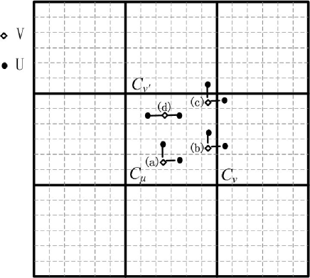
Figure 1: The scheme of spatial coarse graining is plotted. Here, a $18\times 18$ microscopic lattice (see dash-line) is divided into a $3\times 3$ CG lattice(see solid-line) by uniformly grouping $6\times 6$ microscopic sites to a CG cell. At the microscopic level, the reaction $2U+V\rightarrow 3U$ can only take place on orthogornal UVU configurations (a), (b) and (c), but not on line configuration (d).

II.4 The CG-KMC Methods

In the present work, we adopt a CG procedure originally introduced by Vlachos et.al Vlachos3 . Since the diffusion processes are usually faster than other slow processes, it is reasonable to assume that particles are well-mixed in a comparatively large domain, whose scale is determined by the diffusion length, over short time scales. Therefore, one can divide the micro-lattice into several coarse cells, wherein each particle is assumed to have an equal probability of occupying any microscopic lattice site, and no spatial correlation exists. Obviously, the most natural way for such a spatial coarse graining on 2D surface is to group $m\times m$ sites into a CG cell. For instance, Fig.1 shows the coarse-graining of a $18\times 18$ micro-lattice into a $3\times 3$ CG-lattice, wherein each CG-cell contains $m^{2}=36$ sites (hereafter, we use ’site’ for the micro-lattice and ’cell’ for the CG-lattice).

To perform CG-KMC, one needs to define the CG processes taking place on the CG lattice and obtain the corresponding CG rates. We now introduce the CG variables

$$\eta^{\phi}_{\mu}=\sum_{i\in C_{\mu}}\sigma^{\phi}_{i}\ \ \ \text{and}\ \ \ \bar{\eta}^{\phi}_{\mu}=\eta^{\phi}_{\mu}/m^{2}$$

to denote the number and coverage of $\phi$-species in the $\mu$-th CG-cell $C_{\mu}$, respectively. Consider the micro-process (1), for example, the CG process is defined as the adsorption of one $U$ particle in any site $i$ inside a CG-cell $C_{\mu}$. Since $U$-adsorption only involves one surface site, there is no spatial correlation between different adsorption events inside a cell, therefore the rate of the CG adsorption process easily reads

$$w_{\mu 1}=\sum_{i\in C_{\mu}}K_{1}(1-\sigma_{i}^{U}-\sigma_{i}^{V})=m^{2}K_{1}(1-\bar{\eta}^{U}_{\mu}-\bar{\eta}^{V}_{\mu}).$$

Following this simple rule, one can readily obtain the CG rates for the single-site processes (1) to (4).

For the diffusion processes (6) and (7), one must bear in mind that the diffusion constant between two adjacent CG-cell, $\tilde{K}_{6}$ ( $\tilde{K}_{7}$ ), is not identical to that between two adjacent micro-sites, $K_{6}(K_{7})$. To establish the relationship between these two rates, we can adopt the so-called ’flux-consistency’ rule, which requires that the average flux across the boundary of two adjacent CG cells, calculated from the CG diffusion process, should be the same as that calculated from averaging over the micro-diffusion process. By using this criterion and considering the maintenance of detail-balance, see Vlachos2 , one must have $\tilde{K}_{6}=K_{6}/m^{2}$ and $\tilde{K}_{7}=K_{7}/m^{2}$. Finally, the rate for the CG diffusion process of $U$ is

$$w_{\mu 6}=\sum_{i}\tilde{K}_{6}\langle\sigma_{i}^{U}(1-\sigma_{j}^{U}-\sigma_{j}^{V})\rangle_{i\in C_{\mu},j\in C_{\nu}}=\frac{K_{6}}{m^{2}}\eta_{\mu}^{U}(1-\bar{\eta}_{\nu}^{U}-\bar{\eta}_{\nu}^{V}).$$

Herein, $\langle\cdot\rangle$ means ensemble average. In the final equation, we have ignored the correlation between different cells and simply replaced the ensemble average of $\sigma_{i}^{\phi}$ inside $C_{\mu}$ by $\bar{\eta}_{\mu}^{\phi}$ Vlachos1 ; Vlachos2 . The rate for CG diffusion of $V$ can be obtained in a similar way.

For the trimolecular reaction process (5), however, strong correlation exists between neighboring sites. To perform the CG simulation, we need to express the ensemble-averaged rate of this process inside a cell by a function of the CG-variables,

$$w_{\mu 5}=F(K_{5},m,\bar{\eta}_{\mu}^{U},\bar{\eta}_{\mu}^{V}).$$

However, it is hard to decide the correct functional form at this stage. It is worthy to note here that a seamless approach has been proposed very recently to address the validity of reaction-diffusion master equationsPNAS . The authors argued that to make the master equation to be consistent with the micro-model, the reaction constant must be dependent on the coarse-size, here is $m$. They demonstrated the success of this idea for a reversible aggregation-dissociation reaction. Unfortunately, it is rather difficult for us to work out a similar result for the trimolecular lattice gas system considered here. Therefore, to step forward, we have to make some approximations. To the lowest order, one may use the simple local mean field (s-LMF) approximation as follows,

$$w_{\mu 5}=m^{2}\langle K_{5}\sigma_{i}^{V}\sigma_{j}^{U}\sigma_{k}^{U}\rangle^{\prime}_{i,j,k\in C_{\mu}}=m^{2}K_{5}\bar{\eta}_{\mu}^{V}(\bar{\eta}_{\mu}^{U})^{2}.$$

Herein, $\langle\cdot\rangle^{\prime}$ denotes the ensemble average over the orthogonal configurations inside $C_{\mu}$. Given that the diffusion process is fast and the cell size is smaller than the diffusion length, this approximation, although crude, might be acceptable.

Unfortunately, as we will show(see below), however, this s-LMF scheme for the reaction process almost fails to reproduce the KMC results, no matter how large the coarse-size $m$ and the diffusion constants $K_{6}(K_{7})$ are. It seems that the s-LMF loses some key components that should be considered during the CG procedure. We note here that the s-LMF scheme totally ignores the correlations between adjacent cells resulted from the trimolecular process. For instance, the reaction configuration (b) (see in Fig.1) on the border of cell $\mu$ involves two sites ($U$ and $V$) in cell $\mu$ and one site ($U$) in cell $\nu$. If we use LMF for both cell $\mu$ and $\nu$, the ensemble averaged rate for this particular configuration should read $K_{5}\bar{\eta}^{U}_{\mu}\bar{\eta}^{V}_{\mu}\bar{\eta}^{U}_{\nu}$, which is different from the rate for the reaction inside $C_{\mu}$, $K_{5}(\bar{\eta}^{U}_{\mu})^{2}\bar{\eta}^{V}_{\mu}$, if we consider that concentration gradients exist between adjacent cells. We argue that this effect should be taken into account to compensate the discrepancy resulted from the CG approximation. Similarly, the reaction configuration (c)(in Fig. 1) at the corner of cell $\mu$ involves sites in three adjacent cells. Therefore, instead of the s-LMF, one may use a boundary-corrected LMF (b-LMF) scheme by writing down the CG-rate of process (5) as follows,

$$w^{b}_{\mu 5}=f_{1}\tilde{w}_{intra}+f_{2}\tilde{w}_{border}+f_{3}\tilde{w}_{corner}.$$ (12)

Herein,

$$\tilde{w}_{intra}=m^{2}K_{5}\bar{\eta}^{V}_{\mu}(\bar{\eta}^{U}_{\mu})^{2},$$ (13)

$$\tilde{w}_{border}=m^{2}K_{5}\bar{\eta}^{V}_{\mu}\bar{\eta}^{U}_{\mu}(\sum_{\nu}\bar{\eta}^{U}_{\nu}/4),$$ (14)

and

$$\tilde{w}_{corner}=m^{2}K_{5}\bar{\eta}^{V}_{\mu}(\sum_{\nu\nu^{\prime}}\bar{\eta}^{U}_{\nu}\bar{\eta}^{U}_{\nu^{\prime}}/4)$$ (15)

denote the average rate of process (5) inside, on the border of, and at the corner of cell $\mu$, respectively. Note that the summation in equation (14) runs over the four adjacent cells of $C_{\mu}$, and that in (15) runs over adjacent cells of the four corners. The weighting factors $f_{1}$, $f_{2}$ and $f_{3}$ denote the possibility of finding an reaction $UVU$ configuration belonging to the three categories, respectively, given that the $V$ site is inside the current cell $C_{\mu}$. By simple manipulations, we have

$$f_{1}=(1-1/m)^{2},\ f_{3}=1/m^{2},\ \ \texttt{and}\ \ f_{2}=1-f_{1}-f_{3}.$$

Table 2: CG processes and rates associated with the CG cell $C_{\mu}$.

Process Description	State Change	$s$-LMF Rate	$b$-LMF Rate
U Adsorption	$\eta^{U}_{\mu}\rightarrow\eta^{U}_{\mu}+1$	${w}_{\mu 1}=m^{2}{K}_{1}(1-\bar{\eta}^{U}_{\mu}-\bar{\eta}^{V}_{\mu})$	${w}_{\mu 1}$
U Desorption	$\eta^{U}_{\mu}\rightarrow\eta^{U}_{\mu}-1$	$w_{\mu 2}=m^{2}{K}_{2}\bar{\eta}^{U}_{\mu}$	$w_{\mu 2}$
U Conversion to V	$\eta^{U}_{\mu}\rightarrow\eta^{U}_{\mu}-1$, $\eta^{V}_{\mu}\rightarrow\eta^{V}_{\mu}+1$	$w_{\mu 3}=m^{2}{K}_{3}\bar{\eta}^{U}_{\mu}$	$w_{\mu 3}$
V Desorption	$\eta^{V}_{\mu}\rightarrow\eta^{V}_{\mu}-1$	$w_{\mu 4}=m^{2}{K}_{4}\bar{\eta}^{V}_{\mu}$	$w_{\mu 4}$
2U+V Reaction	$\eta^{V}_{\mu}\rightarrow\eta^{V}_{\mu}-1$, $\eta^{U}_{\mu}\rightarrow\eta^{U}_{\mu}+1$	$w_{\mu 5}=m^{2}{K}_{5}\bar{\eta}^{V}_{\mu}(\bar{\eta}_{\mu}^{U})^{2}$	$w_{\mu 5}^{b}$
U Diffusion	$\eta^{U}_{\mu}\rightarrow\eta^{U}_{\mu}-1$, $\eta^{U}_{\nu}\rightarrow\eta^{U}_{\nu}+1$	$w_{\mu 6}={K}_{6}\bar{\eta}^{U}_{\mu}(1-\bar{\eta}^{U}_{\nu}-\bar{\eta}^{V}_{\nu})$	$w_{\mu 6}$
V Diffusion	$\eta^{V}_{\mu}\rightarrow\eta^{V}_{\mu}-1$,$\eta^{V}_{\nu}\rightarrow\eta^{V}_{\nu}+1$	$w_{\mu 7}={K}_{7}\bar{\eta}^{V}_{\mu}(1-\bar{\eta}^{U}_{\nu}-\bar{\eta}^{V}_{\nu})$	$w_{\mu 7}$

In Table II, the CG processes as well as their corresponding CG rates are listed. Note that b-LMF and s-LMF show difference only for the trimolecular reaction. According to these processes and rates, one can readily perform CG-KMC simulations. In the present paper, we also use null-event procedure as that for the KMC. The steps are outlined as follows,

1. Choose a process similar to the first step used in the KMC, except that now $K_{6}$ and $K_{7}$ should be replaced by $\tilde{K}_{6}=K_{6}/m^{2}$ and $\tilde{K}_{7}=K_{7}/m^{2}$. Correspondingly, $W_{0}$ should be changed to $W^{CG}_{0}$.

2. Randomly select a cell $\mu$ with equal probability.

3. Calculate the reaction probability $\epsilon_{\mu\alpha}$ for the process $\alpha$ to happen associated with the current cell $\mu$. This probability simply equals to $w_{\mu\alpha}/(K_{\alpha}m^{2})$ for $1\leq\alpha\leq 5$ and $w_{\mu\alpha}/(\tilde{K}_{\alpha}m^{2})$ for $\alpha=6$ or 7.

4. Generate a second uniformly distributed random number $r_{2}$ in the unit interval. If $r_{2}\leq\epsilon_{\mu\alpha}$, execute the process $\alpha$, and the trial ends otherwise.

5. Repeat the above steps.

In the present study, we start CG-KMC simulations from the same initial conditions as in the KMC. To be consistent with the KMC, the time increment should read $\tau_{CG}=1/W^{CG}_{0}$ for each trial. We compare the CG-KMC results with the KMC ones to check the validity of CG approaches.

III Numerical Simulations and Discussion

In our work, the main parameters used in simulations are $K_{1}=5.0\times 10^{-5}$, $K_{2}=1.0\times 10^{-3}$, $K_{3}=5.0\times 10^{-3}$ and $K_{4}=6.0\times 10^{-5}$, while $K_{5}$ and $K_{6}=K_{7}=D$ are control parameters. To compare the results of different methods, we have generated time series $u(t)$ or $v(t)$ with enough length and calculated the oscillation amplitude $A$ and period $T$ as a function of the control parameters. In Fig.(2a), the dependence of the oscillation range of $v$ on $K_{5}$ is shown, obtained by the MFDE, CLE and KMC with different diffusion constant $D$. Correspondingly the curves for the period $T$ are drawn in Fig.(2b). The CLE results are obtained by numerical simulation of Eq.(10) and (11) with a time step $\Delta t=0.01$ and $N=256$. All the KMC results are also performed on a $256\times 256$ square lattice. The solid line obtained from MFDE corresponds to the bifurcation diagram. A Hopf bifurcation locates at $K_{5c}\simeq 2.15$, below which deterministic oscillation can be observed. Several points can be addressed from this figure. First of all, CLE and KMC show strong qualitative differences with the MFDE: Stochastic oscillations can be observed even outside the deterministic oscillatory region, here $K_{5}>K_{5c}$. This so-called noise induced oscillation phenomenon has gained great attention in recent years and may have important applications especially in circadian oscillation systems. Secondly, the KMC results depend strongly on the diffusion constant $D$. However, the results for $D=10$ and $D=30$ nearly collapse, indicating that the KMC results may converge in the limit of large $D$. In this latter case, the MFDE can reproduce the KMC results when the parameter lies deep inside the oscillatory region, see the range $K_{5}<2.1$. If $D$ is small, both MFDE and CLE show large discrepancies with the KMC results, no matter the range of the control parameter. Finally, we would like to point out here that the CLE cannot reproduce the KMC results accurately even for large $D$, although they share some qualitative features, e.g., noise induced oscillation to the right side of the Hopf point.

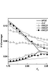
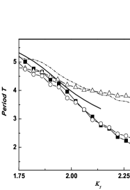
Figure 2: The oscillation range of (a) $V$-coverage and (b) period are presented as functions of control parameter $K_{5}$, obtained by MFDE, CLE and KMC with $D=1,10,30$, respectively. Parameters are $K_{1}=5.0\times 10^{-5}$, $K_{2}=1.0\times 10^{-3}$, $K_{3}=5.0\times 10^{-3}$, $K_{4}=6.0\times 10^{-5}$ and $N=256$.

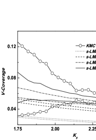
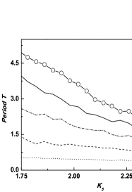
Figure 3: The oscillation range of (a) $V$-coverage and (b) period obtained from the $s$-LMF CG approach with different coarse size $m$. The diffusion constant is $D=10$ and the other parameters are the same as in Fig. 2.

In the following part, we mainly consider a system with size $N=256$ and diffusion constant $D=10$. We have also performed some KMC simulations on larger systems, e.g., $N=512$, but the main conclusions are the same. Since we are mainly interested in the validity of CG methods and extensive simulations are required to compare the results of different methods, we have fixed $N=256$ throughout the paper. CG-KMC simulations are performed according to the CG processes and rates listed in Table II. In Fig.3, the oscillation amplitude and period obtained by using s-LMF rates are shown, for different sizes of the CG cell. Apparently, the s-LMF approach almost fails to reproduce the results of KMC, even qualitatively. For small $m$, the s-LMF totally loses the whole bifurcation features of the KMC dynamics. We show in Fig.4, however, that the b-LMF behaves much better than the s-LMF. Firstly, the b-LMF can reproduce the global bifurcation feature quite well, even for small $m$. In addition, for an intermediate value of $m$, say, $m=8$ here, the b-LMF results show excellent consistent with the KMC results, in both the oscillation amplitude (Fig.4a) and the period (Fig.4b). It seems that the b-LMF approach does catch some key factors during the CG procedure.

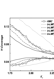
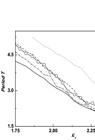
Figure 4: The oscillation range of (a) $V$-coverage and (b) period obtained from the $b$-LMF CG approach with different coarse size $m$. The diffusion constant is $D=10$ and the other parameters are the same as in Fig. 2.

In Fig.5, we have plotted the dependence of the turnover frequency (TOF) as a function of time for different coarse size $m$ obtained from the KMC, b-LMF and s-LMF. The TOF is defined as the occurrence of the trimolecular reaction (5) per surface site per unit time. Clearly, the b-LMF with $m=8$ matches the KMC quite well, while that with smaller or larger $m$ may capture some qualitative features of the TOF but with apparent quantitative differences. The s-LMF, however, almost loses the temporal information associated with the TOF.

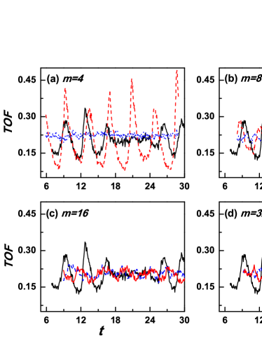
Figure 5: The dependence of TOF as a function of time on the coarse cell size $m$ obtained from the KMC(solid-line), $b$-LMF(dash-line) and $s$-LMF(dot-line), respectively.

To further demonstrate this quantitatively, we introduce a deviation coefficient for the oscillation range as follows. According to Fig.3 and Fig.4, each bifurcation diagram contains two branches, the upper branch and the lower one corresponding to the averaged maximum and minimum values of $v(t)$, respectively. As can be seen from the figures, both branches obtained from the CG-KMC methods show discrepancies with the KMC values. Denote the upper branch value of $v$, obtained by CG-KMC, at a certain control parameter $K_{5}$ by $v^{u}_{k}$, and that obtained by KMC by $v^{u}_{k0}$, then

$$\gamma^{u}_{A}=\frac{1}{2N_{k}}\sum_{k}\frac{|v^{u}_{k}-v^{u}_{k0}|}{v^{u}_{k0}}$$

measures the relative discrepancy of the upper branch, where $N_{k}$ is the number of control parameters used in the calculation. Similarly, we can calculate the discrepancy of the lower branch $\gamma^{l}_{A}$. In the present work, we have used $N_{k}=20$ points inside the range $K_{5}\in(1.75,2.5)$ to obtain $\gamma^{u}_{A}$ and $\gamma^{l}_{A}$. In Fig.(6a), the dependence of $\gamma_{A}=(\gamma^{u}_{A}+\gamma^{l}_{A})/2$ on the size $m$ of CG-cell is shown, for the b-LMF with different diffusion constant $D$ and the s-LMF with $D=10$. In Fig.(6b), the curves for $\gamma_{T}$, the relative discrepancy in the period, are shown. Clearly, the s-LMF method shows relatively large discrepancies, while the b-LMF works much better. The s-LMF is even worse than the MFDE, shown by the dash lines in Fig.6 for $D=10$. One notes that both $\gamma_{A}$ and $\gamma_{T}$ exhibit a clear-cut minimum of about zero at $m=8$ for large $D$ when b-LMF is used. We also note that if $D$ is small, say $D=1$ here, the b-LMF also fails. This is not surprising because CG method which assumes well-mixing in a CG-cell should not work if diffusion is too slow.

In the above results, we see that the CG results for small $m$ do not match the results of KMC, even for the b-LMF. This is in contrast to the CG-KMC methods used by Vlachos et.al to account for the dynamics of 2D lattice gas Ising model. Note that for the Ising model, one mainly considered the equilibrium states. For the Brusselator model considered here, however, we want to reproduce the temporal oscillation behavior. To reproduce the oscillation features on the whole surface, the temporal correlation of the time series must be properly maintained during the CG procedure. When we perform the CG procedure by dividing the lattice into CG cells, we are dealing with $N^{c}\times N^{c}$ coupled CG oscillators, where $N^{c}=N/m$ is the size of the CG lattice. The coupling between these CG oscillators are realized by the diffusion and the boundary correlation considered in the b-LMF. If the CG cell is too small, however, the time-correlation inside each cell will be lost due to strong fluctuations and the time evolution of $\eta^{\phi}(t)$ cannot be viewed as an oscillation. As discussed by P.Gaspard, a minimum number of well-mixed molecules is required to produce correlated oscillations, such that the auto-correlation time of the time series is not smaller than $T/2\pi$Gaspard ; Zhadnov2001 . Therefore, it seems that a seamless CG approach to reproduce temporal dissipative structures like chemical oscillation is a large challenge. On the other hand, for any CG method within LMF scheme to work well, the scale of a CG cell should not be larger than the diffusion length, as emphasized by Mikhailov and othersMik0 ; Vlachos2 . The compromise between these two factors, i.e., to keep time autocorrelation and to be smaller than the diffusion length, may be the reason of appearance of an optimal $m$ for the b-LMF approach. We note that this reasoning is not applicable to the s-LMF, for which the discrepancies monotonically decrease with increasing $m$, since the s-LMF does not work for the present system.

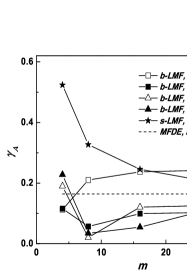
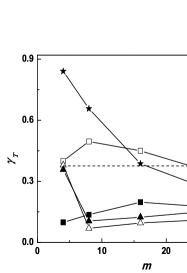
Figure 6: The dependence of the deviation coefficient (a) for the oscillation amplitude $\gamma_{A}$ and (b) oscillation period $\gamma_{T}$ on the coarse cell size $m$ obtained from the $s$-LMF and $b$-LMF methods. Parameter are the same as in Fig. 2 and $N=256$.

IV Conclusions

In summary, we have tried to apply a CG-KMC approach to simulate the oscillation behavior on the surface lattice-gas Brusselator model. Owing to the correlations between adjacent cells resulted from the nonlinear trimolecular reaction, the CG approach based on simple LMF approximation almost fails. By properly taking into account the boundary corrections, we have introduced a so-called b-LMF CG-KMC approach, which can reproduce the microscopic KMC results quite well, given that the diffusion is not too slow and the CG cell size is optimally chosen. Our work thus unravels the very role of reaction correlations which should be carefully considered in any CG approach and mesoscopic modeling for nonequilibrium spatiotemporal dynamics at nanoscales.

- (1) A. S. Mikhailov and G. Ertl, Chem. Phys. Chem. 10, 86 (2009).
- (2) M. Hildebrand, M. Ipsen, A. S. Mikhailov and G. Ertl, New J. Phys. 54, 61(2003).
- (3) Y. De Decker and A. S. Mikhailov, J. Phys. Chem. B 108, 14759(2004).
- (4) Y. De Decker and A. S. Mikhailov, Prog. Theo. Phys. Supp. 165, 119 (2006).
- (5) C. Sachs, M. Hildebrand, S. Volkening, J. Wintterlin and G. Ertl, Science 293, 1635 (2001).
- (6) T. Zambelli, J. V. Barth, J. Wintterlin and G. Ertl, Nature 390, 495 (1997).
- (7) S. Jakubith, H. H. Rotermund, W. Engel, A. von Oertzen and G. Ertl, Phys. Rev. Lett. 65, 3013 (1990).
- (8) J. Wintterlin, S. Völkening, T. V. W. Janssens, T. Zambelli and G. Ertl, Science 278, 1931(1997).
- (9) M. Gruyters, D. A.King, J. Chem. Soc. 93, 2947(1997).
- (10) M. M. Slinko, N. I. Jaeger, Oscillatory Heterogeneous Catalytic Systems, Elsevier, Amsterdam, 1994.
- (11) E. E. Mola, I. M. Irurzun, J. L. Vicente and D. A. King, Surf. Rev. Lett. 10, 23(2003).
- (12) F. Schüth, B. E. Henry and L. D. Schmidt, Adv. Catal. 39, 51 (1993).
- (13) A. Provata and V. K. Noussiou, Phys. Rev. E 72, 066108 (2005).
- (14) V. P. Zhdanov and T. Matsushima, Surf. Sci. 583 253(2005).
- (15) V. P. Zhdanov, Surf. Sci. Rep. 45, 231 (2002).
- (16) V. P. Zhdanov and B. Kasemo, Surf. Sci. Rep. 39, 25(2000).
- (17) V. P. Zhdanov and T. Matsushima, Phys. Rev. Lett 98, 036101(2007).
- (18) V. P. Zhdanov, J. Chem. Phys. 126, 074706(2007).
- (19) M. Hildebrand and A. S. Mikhailov, J. Phys. Chem. 100, 19089(1996).
- (20) M. Hildebrand, A. S. Mikhailov and G. Ertl, Phys. Rev. E 58, 5483(1998).
- (21) M. Hildebrand, A. S. Mikhailov and G. Ertl, Phys. Rev. Lett. 81, 2602(1998).
- (22) M. Hildebrand, Chaos 12, 144(2002).
- (23) M. Hildebran and A. S. Mikhailov, J. Stat. Phys. 101, 599(2000).
- (24) A. S. Mikhailov, M. Hildebrand and G. Ertl, in Coherent Structures in Complex Systems, Springer, New York, 252(2001)
- (25) A. Chatterjee and D. G. Valchos, J. Chem. Phys. 124, 064110 (2006).
- (26) M. A. Katsoulakis and D. G. Vlachos, J. Chem. Phys. 119, 9412 (2003).
- (27) A. Chatterjee and D. G. Vlachos, J. Chem. Phys. 121, 11420 (2004).
- (28) M. A. Katsoulakis, A. J. Majda and D. G. Vlachos, J. Comput. Phys. 186, 250 (2003).
- (29) M. A. Katsoulakis, A. J. Majda and D. G. Vlachos, Proc. Natl. Acad. Sci. 100, 782 (2003).
- (30) A. Chatterjee and D. G. Vlachos, Chem. Eng. Sci. 62, 4852(2007).
- (31) S. D. Collins, A. Chatterjee and D. G. Vlachos, J. Chem. Phys. 129, 184101(2008).
- (32) S. D. Collins, M. Stamatakis and D. G. Vlachos, BMC Bioinformatics 11, 218(2010).
- (33) R. Imbihl and G. Ertl, Chem. Rev. 95, 697 (1995).
- (34) A. Chatterjee and D. G. Vlachos, J. Comput.-Aided Mater Des 14, 253 (2007).
- (35) V.P. Zhdanov, Phys. Chem. Chem. Phys. 3, 1432(2001).
- (36) D. Fange, O. G. Berg, P. Sjöberg and J. Elf, Proc. Natl. Acad. Sci., 107, 19820(2010).
- (37) P. Gaspard, J. Chem. Phys. 117, 8905 (2002).