Anderson Orthogonality and the Numerical Renormalization Group

Abstract

Anderson Orthogonality (AO) refers to the fact that the ground states of two Fermi seas that experience different local scattering potentials, say $|G_{\rm I}\rangle$ and $|G_{\rm F}\rangle$, become orthogonal in the thermodynamic limit of large particle number $N$, in that $|\langle G_{\rm I}|G_{\rm F}\rangle|\sim N^{-\frac{1}{2}\Delta_{\mathrm{AO}}^{2}}$ for $N\to\infty$. We show that the numerical renormalization group offers a simple and precise way to calculate the exponent $\Delta_{\mathrm{AO}}$: the overlap, calculated as function of Wilson chain length $k$, decays exponentially, $\sim e^{-k\alpha}$, and $\Delta_{\mathrm{AO}}$ can be extracted directly from the exponent $\alpha$. The results for $\Delta_{\mathrm{AO}}$ so obtained are consistent (with relative errors typically smaller than 1%) with two other related quantities that compare how ground state properties change upon switching from $|{\rm G}_{\rm I}\rangle$ to $|{\rm G}_{\rm F}\rangle$: the difference in scattering phase shifts at the Fermi energy, and the displaced charge flowing in from infinity. We illustrate this for several nontrivial interacting models, including systems that exhibit population switching.

I Introduction

In 1967, Anderson considered the response of a Fermi sea to a change in local scattering potential and made the following observation: Anderson (1967) the ground states $|G_{\rm I}\rangle$ and $|G_{\rm F}\rangle$ of the Hamiltonians ${\hat{H}_{\rm I}}$ and ${\hat{H}_{\rm F}}$ describing the system before and after the change, respectively, become orthogonal in the thermodynamic limit, decaying with total particle number $N$ as

$$|\langle G_{\rm I}|G_{\rm F}\rangle|\sim N^{-\frac{1}{2}\Delta_{\mathrm{AO}}^{2}}\;,$$ (1)

because the single-particle states comprising the two Fermi seas are characterized by different phase shifts.

Whenever the Anderson orthogonality (AO) exponent $\Delta_{\mathrm{AO}}$ is finite, the overlap of the two ground state wave functions goes to zero as the system size becomes macroscopic. As a consequence, matrix elements of the form $|\langle G_{{\rm I}}|\hat{\mathcal{O}}|G_{{\rm F}}\rangle|$, where $\hat{\mathcal{O}}$ is a local operator acting at the site of the localized potential, necessarily also vanish in the thermodynamic limit. This fact has far-reaching consequences, underlying several fundamental phenomena in condensed matter physics involving quantum impurity models, i.e. models describing a Fermi sea coupled to localized quantum degrees of freedom. Examples are the Mahan exciton (ME) and the Fermi-edge singularity (FES) Mahan (1967); Schotte and Schotte (1969b, a); Nozières et al. (1969) in absorption spectra, and the Kondo effect Yuval and Anderson (1970) arising in magnetic alloys Kondo (1964) or in transport through quantum dots. Goldhaber-Gordon et al. (1998) For all of these, the low-temperature dynamics is governed by the response of the Fermi sea to a sudden switch of a local scattering potential. More recently, there has also been growing interest in inducing such a sudden switch, or quantum quench, by optical excitations of a quantum dot tunnel-coupled to a Fermi sea, in which case the post-quench dynamics leaves fingerprints, characteristic of AO, in the optical absorption or emission line shape. Helmes et al. (2005); Türeci et al. (2009); Latta et al. (2009)

The intrinsic connection of local quantum quenches to the scaling of the Anderson orthogonality with system size can be intuitively understood as follows. Consider an instantaneous event at the location of the impurity at time $t=0$ in a system initially in equilibrium. This local perturbation will spread out spatially, such that for $t>0$, the initial wave function is affected only within a radius $L\simeq v_{f}t$ of the impurity, with $v_{f}$ the Fermi velocity. The AO finite-size scaling in Eq. (1) therefore directly resembles the actual experimental situation, and in particular allows the exponent $\Delta_{\mathrm{AO}}$ to be directly related to the exponents seen in experimental observables at long time scales, or at the threshold frequency in Fourier space.Muender2011b

A powerful numerical tool for studying quantum impurity models is the numerical renormalization group (NRG),Wilson (1975); Bulla et al. (2008) which allows numerous static and dynamical quantities to be calculated explicitly, also in the thermodynamic limit of infinite bath size. The purpose of the present paper is to point out that NRG also offers a completely straightforward way to calculate the overlap $|\langle G_{\rm I}|G_{\rm F}\rangle|$ and hence to extract $\Delta_{\mathrm{AO}}$. The advantage of using NRG for this purpose is that NRG is able to deal with quantum impurity models that in general also involve local interactions, which are usually not tractable analytically. Although Anderson himself did not include local interactions in his considerations,Anderson (1967) his prediction (1) still applies, provided the ground states $|G_{{\rm I},{\rm F}}\rangle$ describe Fermi liquids. This is the case for most impurity models (but not all; the two-channel Kondo model is a notable exception). Another useful feature of NRG is that it allows consistency checks on its results for overlap decays, since $\Delta_{\mathrm{AO}}$ is known to be related to a change of scattering phase shifts at the Fermi surface. These phase shifts can be calculated independently, either from NRG energy flow diagrams, or via Friedel’s sum rule from the displaced charge, as will be elaborated below.

A further concrete motivation for the present study is to develop a convenient tool for calculating AO exponents for quantum dot models that display the phenomenon of population switching. Silvestrov and Imry (2000); Golosov and Gefen (2006); Karrasch et al. (2007); Goldstein et al. (2010) In such models, a quantum dot tunnel-coupled to leads contains levels of different widths, and is capacitively coupled to a gate voltage that shifts the levels energy relative to the Fermi level of the leads. Under suitable conditions, an (adiabatic) sweep of the gate voltage induces an inversion in the population of these levels (a so called population switch), implying a change in the local potential seen by the Fermi seas in the leads. In this paper, we verify that the method of extracting $\Delta_{\mathrm{AO}}$ from $\langle G_{\rm I}|G_{\rm F}\rangle$ works reliably also for such models. In a separate publication Muender2011b we will use this method to analyze whether AO can lead to a quantum phase transition in such models, as suggested in Ref. Goldstein et al., 2010.

The remainder of this paper is structured as follows: In Sec. II we define the AO exponent $\Delta_{\mathrm{AO}}$ in general terms, and explain in Sec. III how NRG can be used to calculate it. Sec. IV presents numerical results for several interacting quantum dot models of increasing complexity: first the spinless interacting resonant level model (IRLM), then the single-impurity Anderson model (SIAM), followed by two models exhibiting population switching, one for spinless, the other for spinful electrons. In all cases, our results for $\Delta_{\mathrm{AO}}$ satisfy all consistency checks to within less than 1%.

II Definition of Anderson orthogonality

II.1 AO for a single channel

To set the stage, let us review AO in the context of a free Fermi sea involving a single species or channel of noninteracting electrons experiencing two different local scattering potentials. The initial and final systems are described in full by the Hamiltonians ${\hat{H}_{\rm I}}$ and ${\hat{H}_{\rm F}}$, respectively. Let $\hat{c}_{\varepsilon,{X}}^{\dagger}|0\rangle$ be the single-particle eigenstates of ${\hat{H}_{X}}$ characterized by the scattering phase shifts $\delta_{X}(\varepsilon)$, where ${X}\in\{{\rm I},{\rm F}\}$ and $\hat{c}_{\varepsilon,{X}}^{\dagger}$ are fermion creation operators, and let $\varepsilon^{f}$ be the same Fermi energy for both Fermi seas $|G_{{X}}\rangle$. Anderson showed that in the thermodynamic limit of large particle number, $N\to\infty$, the overlap

$$\left\langle G_{{\rm I}}|G_{{\rm F}}\right\rangle=\left\langle 0\right|\prod_{\varepsilon<\varepsilon^{f}}\hat{c}_{\varepsilon,{\rm I}}^{\ }\cdot\prod_{\varepsilon<\varepsilon^{f}}\hat{c}_{\varepsilon,{\rm F}}^{\dagger}\left|0\right\rangle$$ (2)

decays as in Eq. (1), Anderson (1967); Schotte and Schotte (1969a) where $\Delta_{\mathrm{AO}}$ is equal to the difference in single-particle phase shifts at the Fermi level,

$$\Delta_{\mathrm{AO}}=\Delta_{\mathrm{ph}}\equiv[\delta_{{\rm F}}(\varepsilon^{f})-\delta_{{\rm I}}(\varepsilon^{f})]/\pi\;.$$ (3)

The relative sign between $\Delta_{\mathrm{AO}}$ and $\Delta_{\mathrm{ph}}$ ($+$, not $-$) does not affect the orthogonality exponent $\Delta_{\mathrm{AO}}^{2}$, but follows standard convention [Ref. Friedel, 1956, Eq. (7), or Ref. Langreth, 1966, Eq. (21)].

In this paper we will compare three independent ways of calculating $\Delta_{\mathrm{AO}}$. (i) The first approach calculates the overlap $|\langle G_{\rm I}|G_{\rm F}\rangle|$ of Eq. (1) explicitly as a function of (effective) system size. The main novelty of the present paper is to point out that this can easily be done in the framework of NRG, as will be explained in detail in section III.

(ii) The second approach is to directly calculate $\Delta_{\mathrm{ph}}$ via Eq. (3), since the extraction of phase shifts $\delta_{X}(\varepsilon^{f})$ from NRG finite-size spectra is well-known: Wilson (1975) provided that ${\hat{H}_{X}}$ describes a Fermi liquid, the (suitably normalized) fixed point spectrum of NRG can be reconstructed in terms of equidistant free-particle levels shifted by an amount determined by $\delta_{X}(\varepsilon^{f})$. The many-body excitation energy of an additional particle, a hole and a particle-hole pair thus allow the phase shift $\delta_{X}(\varepsilon^{f})$ to be determined unambiguously.

(iii) The third approach exploits Friedel’s sum rule,Friedel (1956) which relates the difference in phase shifts to the so called displaced charge $\Delta_{\mathrm{ch}}$ via $\Delta_{\mathrm{ch}}=\Delta_{\mathrm{ph}}$. Here the displaced charge $\Delta_{\mathrm{ch}}$ is defined as the charge in units of $e$ (i.e. the number of electrons) flowing inward from infinity into a region of large but finite volume, say $V_{\rm large}$, surrounding the scattering location, upon switching from ${\hat{H}_{\rm I}}$ to ${\hat{H}_{\rm F}}$:

$$\Delta_{\mathrm{ch}} \equiv \left\langle G_{{\rm F}}\right|\hat{n}_{\mathrm{tot}}\left|G_{{\rm F}}\right\rangle-\left\langle G_{{\rm I}}\right|\hat{n}_{\mathrm{tot}}\left|G_{{\rm I}}\right\rangle$$ (4)

$$\equiv {\Delta_{\mathrm{sea}}}+{\Delta_{\mathrm{dot}}}\;.$$

Here $\hat{n}_{\rm tot}\equiv\hat{n}_{\rm sea}+\hat{n}_{\mathrm{dot}}$, where $\hat{n}_{\mathrm{sea}}$ is the total number of Fermi see electrons within $V_{\rm large}$, whereas $\hat{n}_{\mathrm{dot}}$ is the local charge of the scattering site, henceforth called “dot”.

To summarize, we have the equalities

$$\Delta_{\mathrm{AO}}^{2}=\Delta_{\mathrm{ph}}^{2}=\Delta_{\mathrm{ch}}^{2}\;,$$ (5)

where all three quantities can be calculated independently and straightforwardly within the NRG. Thus Eq. (5) constitutes a strong consistency check. We will demonstrate below that NRG results satisfy this check with good accuracy (deviations are typically below 1%).

II.2 AO for multiple channels

We will also consider models involving several independent and conserved channels (e.g. spin in spin-conserving models). In the absence of interactions, the overall ground state wave function is the product of those of the individual channels. With respect to AO, this trivially implies that each channel adds independently to the AO exponent in Eq. (1),

$$\Delta_{\mathrm{AO}}^{2}=\sum_{\mu=1}^{{N_{\mathrm{c}}}}{\Delta_{\mathrm{AO}}^{2}}_{,\mu}\text{,}$$ (6)

where $\mu=1,\ldots,{N_{\mathrm{c}}}$ labels the ${N_{\mathrm{c}}}$ different channels. We will demonstrate below that the additive character in Eq. (6) generalizes to systems with local interactions, provided that the particle number in each channel remains conserved. This is remarkable, since interactions may cause the ground state wave function to involve entanglement between local and Fermi sea degrees of freedom from different channels. However, our results imply that the asymptotic tails of the ground state wave function far from the dot still factorize into a product of factors from individual channels. In particular, we will calculate the displaced charge for each individual channel, cf. Eq. (4),

$$\Delta_{{\mathrm{ch}},\mu} \equiv \left\langle G_{{\rm F}}\right|\hat{n}_{{\mathrm{tot}},\mu}\left|G_{{\rm F}}\right\rangle-\left\langle G_{{\rm I}}\right|\hat{n}_{{\mathrm{tot}},\mu}\left|G_{{\rm I}}\right\rangle$$ (7)

$$\equiv {{\Delta_{\mathrm{sea}}}}_{,\mu}+{{\Delta_{\mathrm{dot}}}}_{,\mu}\;,$$

where $\hat{n}_{{\mathrm{tot}},\mu}=\hat{n}_{{\mathrm{sea}},\mu}+\hat{n}_{{\mathrm{dot}},\mu}$. Assuming no interactions in the respective Fermi seas, it follows from Friedel’s sum rule that ${\Delta_{\mathrm{AO}}^{2}}_{,\mu}={\Delta_{\mathrm{ch}}^{2}}_{,\mu}$, and therefore

$$\Delta_{\mathrm{AO}}^{2}=\sum_{\mu=1}^{{N_{\mathrm{c}}}}{\Delta_{\mathrm{ch}}^{2}}_{,\mu}\equiv\Delta_{\mathrm{ch}}^{2}\,,$$ (8)

where $\Delta_{\mathrm{ch}}^{2}$ is the total sum of the squares of the displaced charges of the separate channels. Equation (8) holds with great numerical accuracy, too, as will be shown below.

III Treating Anderson Orthogonality using NRG

III.1 General impurity models

The problem of a noninteracting Fermi sea in the presence of a local scatterer belongs to the general class of quantum impurity models treatable by Wilson’s NRG.Wilson (1975) Our proposed approach for calculating $\Delta_{\mathrm{AO}}$ applies to any impurity model treatable by NRG. To be specific, however, we will focus here on generalized Anderson impurity type models. They describe ${N_{\mathrm{c}}}$ different (and conserved) species or channels of fermions that hybridize with local degrees of freedom at the dot, while all interaction terms are local.

We take both the initial and final ($X\in\{{\rm I},{\rm F}\}$) Hamiltonians to have the generic form $\hat{H}_{X}={\hat{H}_{\rm b}}+\hat{H}_{{\mathrm{d}},{X}}+\hat{H}_{\textrm{int}}$. The first term,

$${\hat{H}_{\rm b}}=\sum_{\mu=1}^{{N_{\mathrm{c}}}}\sum_{\varepsilon}\varepsilon\,\hat{c}^{\dagger}_{\varepsilon\mu}\hat{c}^{\phantom{\dagger}}_{\varepsilon\mu}\text{,}$$ (9)

describes a noninteracting Fermi sea involving ${N_{\mathrm{c}}}$ channels. (${N_{\mathrm{c}}}$ includes the spin index, if present.) For simplicity, we assume a constant density of states $\rho_{\mu}(\varepsilon)=\rho_{0,\mu}\theta(D-|\varepsilon|)$ for each channel with half-bandwidth $D$. Moreover, when representing numerical results, energies will be measured in units of half-bandwidth, hence $D:=1$. The Fermi sea is assumed to couple to the dot only via the local operators $\hat{f}^{\phantom{\dagger}}_{0\mu}=\tfrac{1}{\sqrt{N_{\rm b}}}\sum_{\epsilon}\hat{c}^{\phantom{\dagger}}_{\epsilon\mu}$ and $\hat{f}^{\dagger}_{0\mu}$, that, respectively, annihilate or create a Fermi sea electron of channel $\mu$ at the position of the dot, $\vec{r}=0$, with a proper normalization constant $N_{\rm b}$ to ensure $[f_{0\mu},f^{\dagger}_{0\mu^{\prime}}]=\delta_{\mu\mu^{\prime}}$.

The second term, $\hat{H}_{{\mathrm{d}},{X}}$, contains the non-interacting local part of the Hamiltonian, including the dot-lead hybridization,

$$\hat{H}_{{\mathrm{d}},{X}} = \sum_{\mu=1}^{{N_{\mathrm{c}}}}\varepsilon_{d\mu,{X}}\hat{n}_{d\mu}+\sum_{\mu=1}^{{N_{\mathrm{c}}}}\sqrt{\tfrac{2\Gamma_{\mu}}{\pi}}\bigl{[}\hat{d}_{\mu}^{{\dagger}}\hat{f}_{0\mu}^{{\phantom{\dagger}}}+h.c.\bigr{]}\text{ .}$$ (10)

Here $\varepsilon_{d\mu,{X}}$ is the energy of dot level $\mu$ in the initial or final configuration, and $\hat{n}_{d\mu}=\hat{d}_{\mu}^{\dagger}\hat{d}_{\mu}$ is its electron number. $\Gamma_{\mu}\equiv\pi\rho_{\mu}V_{\mu}^{2}$ is the effective width of level $\mu$ induced by its hybridization with channel $\mu$ of the Fermi sea, with $V_{\mu}$ the $\mu$-conserving matrix element connecting the d-level with the bath states $\hat{c}_{\varepsilon\mu}$, taken independent of energy, for simplicity.

Finally, the interacting third term is given in the case of the single-impurity Anderson model (SIAM) by the uniform Coulomb interaction $U$ at the impurity,

$$\hat{H}^{\textrm{SIAM}}_{\textrm{int}} = \tfrac{1}{2}U\hat{n}_{\mathrm{d}}(\hat{n}_{\mathrm{d}}-1)\text{,}$$ (11)

with $\hat{n}_{\mathrm{d}}=\sum_{\mu}\hat{n}_{d\mu}$, while in case of the interacting resonant level model (IRLM), the interacting part is given by

$$\hat{H}^{\textrm{IRLM}}_{\textrm{int}} = U^{\prime}\hat{n}_{\mathrm{d}}\hat{n}_{0}\text{ ,}$$ (12)

with $\hat{n}_{0}=\sum_{\mu}f^{\dagger}_{0,\mu}f^{\phantom{\dagger}}_{0,\mu}\equiv\sum_{\mu}\hat{n}_{0,\mu}$. In particular, most of our results are for the one- or two-lead versions of the SIAM for spinful or spinless electrons,

$$\hat{H}^{\textrm{SIAM}}_{X}={\hat{H}_{\rm b}}+\hat{H}_{{\mathrm{d}},{X}}+\hat{H}_{\textrm{int}}^{\textrm{SIAM}}\;.$$ (13)

We consider either a single dot-level coupled to a single lead (spinfull, ${N_{\mathrm{c}}}=2:\ \mu\in\{\uparrow,\downarrow\}$), or a dot with two levels coupled separately to two leads (spinless, ${N_{\mathrm{c}}}=2:\ \mu\in\{1,2\}$; spinfull, ${N_{\mathrm{c}}}=4:\ \mu\in\{1\!\!\uparrow,1\!\!\downarrow,2\!\!\uparrow,2\!\!\downarrow\}$). A splitting of the energies $\varepsilon_{d\mu,{X}}$ in the spin label (if any), will be referred to as magnetic field $B$. We also present some results for the IRLM, for a single channel of spinless electrons (${N_{\mathrm{c}}}=1$):

$$\hat{H}^{\textrm{IRLM}}_{X}={\hat{H}_{\rm b}}+\hat{H}_{{\mathrm{d}},{X}}+\hat{H}_{\textrm{int}}^{\textrm{IRLM}}\;.$$ (14)

In this paper, we focus on the case that $\hat{H}_{\rm I}$ and $\hat{H}_{\rm F}$ differ only in the local level positions ($\varepsilon_{d\mu,{\rm I}}\neq\varepsilon_{d\mu,{\rm F}}$). It is emphasized, however, that our methods are equally applicable for differences between initial and final values of any other parameters, including the case that the interactions are channel-specific, e.g. $\sum_{\mu\mu^{\prime}}U_{\mu\mu^{\prime}}\hat{n}_{d\mu}\hat{n}_{d\mu^{\prime}}$ or $\sum_{\mu\mu^{\prime}}U^{\prime}_{\mu\mu^{\prime}}\hat{n}_{d\mu}\hat{n}_{0\mu^{\prime}}$.

III.2 AO on Wilson chains

Wilson discretized the spectrum of ${\hat{H}_{\rm b}}$ on a logarithmic grid of energies $\pm D\Lambda^{-k}$ (with $\Lambda>1$, $k=0,1,2,\dots$), thereby obtaining exponentially high resolution of low-energy excitations. He then mapped the impurity model onto a semi-infinite “Wilson tight-binding chain” of sites $k=0$ to $\infty$, with the impurity degrees of freedom coupled only to site 0. To this end, he made a basis transformation from the set of sea operators $\{\hat{c}_{\varepsilon\mu}\}$ to a new set $\{\hat{f}_{k\mu}\}$, chosen such that they bring ${\hat{H}_{\rm b}}$ into the tridiagonal form

$${\hat{H}_{\rm b}}\simeq\sum_{\mu=1}^{{N_{\mathrm{c}}}}\sum_{k=1}^{\infty}t_{k}(\hat{f}^{\dagger}_{k\mu}\hat{f}^{{\phantom{\dagger}}}_{k-1,\mu}+{\rm h.c.})\;.$$ (15)

The hopping matrix elements $t_{k}\propto D\Lambda^{-k/2}$ decrease exponentially with site index $k$ along the chain. Because of this separation of energy scales, the Hamiltonian can be diagonalized iteratively by solving a Wilson chain of length $k$ (restricting the sum in Eq. (15) to the first $k$ terms) and increasing $k$ one site at a time: starting with a short Wilson chain, a new shell of many-body eigenstates for a Wilson chain of length $k$, say $|s\rangle_{k}$, is constructed from the states of site $k$ and the $M_{K}$ lowest-lying eigenstates of shell $k-1$. The latter are the so called kept states $|s\rangle_{k-1}^{K}$ of shell $k-1$, while the remaining higher-lying states $|s\rangle_{k-1}^{D}$ from that shell are discarded.

The typical spacing between the few lowest-lying states of shell $k$, i.e. the energy scale $dE_{k}$, is set by the hopping matrix element $t_{k}$ to the previous site, hence

$$dE_{k}\simeq t_{k}\propto D\Lambda^{-k/2}\;.$$ (16)

Now, for a noninteracting Fermi sea with $N$ particles, the mean single-particle level spacing at the Fermi energy scales as $dE\propto D/N$. This also sets the energy scale for the mean level spacing of the few lowest-lying many-body excitations of the Fermi sea. Equating this to Eq. (16), we conclude that a Wilson chain of length $k$ represents a Fermi sea with an actual size $L\propto N$, i.e. an effective number of electrons $N$, that grows exponentially with $k$,

$$N\propto\Lambda^{k/2}\;.$$ (17)

Now consider two impurity models that differ only in their local terms $\hat{H}_{{\mathrm{d}},{X}}$, and let $|G_{X}\rangle_{k}$ be the ground states of their respective Wilson chains of length $k$, obtained via two separate NRG runs. Helmes et al. (2005) Combining Anderson’s prediction (1) and Eq. (17), the ground state overlap is expected to decay exponentially with $k$ as

$$|{}_{k\!\!}\left\langle G_{{\rm I}}|G_{{\rm F}}\right\rangle_{k}|\propto\Lambda^{-k\Delta_{\mathrm{AO}}^{2}/4}\equiv e^{-\alpha k}\,$$ (18)

with

$$\Delta_{\mathrm{AO}}^{2}=\frac{4\alpha}{\log\Lambda}\;.$$ (19)

Thus the AO exponent can be determined by using NRG to directly calculate the l.h.s. of Eq. (18) as function of chain length $k$, and extracting $\Delta_{\mathrm{AO}}$ from the exponent $\alpha$ characterizing its exponential decay with $k$.

For noninteracting impurity models ($U=U^{\prime}=0$), a finite Wilson chain represents a single-particle Hamiltonian for a finite number of degrees of freedom that can readily be diagonalized numerically, without the need for implementing NRG truncation. The ground state is a Slater determinant of those single-particle eigenstates that are occupied in the Fermi sea. The overlap $\langle G_{\rm I}|G_{\rm F}\rangle$ is then given simply by the determinant of a matrix whose elements are overlaps between the ${\rm I}$- and ${\rm F}$-versions of the occupied single-particle states. It is easy to confirm numerically in this manner that $\langle G_{\rm I}|G_{\rm F}\rangle\sim e^{-\alpha k}$, leading to the expected AO in the limit $k\to\infty$. We will thus focus on interacting models henceforth, that require the use of NRG.

In the following three subsections, we discuss several technical aspects needed for calculating AO with NRG on Wilson chains.

III.3 Ground state overlaps

The calculation of state space overlaps within the NRG is straightforward in principleHelmes et al. (2005); Anders and Schiller (2006), especially considering its underlying matrix product state structure Weichselbaum and von Delft (2007); Weichselbaum et al. (2009); Schollwöck (2011). Now, the overlap in Eq. (18) that needs to be calculated in this paper, is with respect to ground states as function of Wilson chain length $k$. As such, two complications can arise. (i) For a given $k$, the system can have several degenerate ground states $\{|s\rangle_{k}^{{X}}:s\in G\}$, with the degeneracy $d_{{X},k}$ typically different for even and odd $k$. (ii) The symmetry of the ground state space may actually differ with alternating $k$ between certain initial and final configurations, ${X}\in\{{\rm I},{\rm F}\}$, leading to strictly zero overlap there. A natural way to deal with (i), is to essentially average over the degenerate ground-state spaces, while (ii) can be ameliorated by partially extending the ground state space to the full kept space, $\{|s\rangle_{k}^{X}:s\in K\}$, as will be outlined in the following.

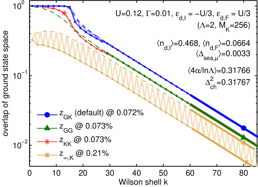
Figure 1: (Color online) Anderson orthogonality for the spin-degenerate standard SIAM for a single lead [Eq. (10), $\mu\in\{\uparrow,\downarrow\}$], with $\mu$-independent parameters $\varepsilon_{{\mathrm{d}}}$ and $\Gamma$ for ${\hat{H}_{\rm I}}$ and ${\hat{H}_{\rm F}}$ as specified in the panel (the full $\varepsilon^{\rm F}_{{\mathrm{d}}}$-dependence of $\Delta_{\mathrm{AO}}$ for fixed $\varepsilon^{\rm I}_{{\mathrm{d}}}$ is analyzed in more detail in Fig. 5) — Several alternative measures for calculating the AO-overlap are shown, using $z_{PP^{\prime}}(k)$ in Eq. (22) with $P^{(\prime)}\in\{G,K,\infty\}$, as defined in the text. All overlaps are plotted for even and odd iterations separately to account for possible even-odd behavior within the Wilson chain (thin solid lines with dots, and dashed lines, respectively, while heavy symbols identify lines with corresponding legends). If even and odd data from the same $z_{PP^{\prime}}(k)$ do not lie on the same smooth line, the combined data is also plotted (light zigzag lines) as guides to the eye. For large $k$, all AO-overlaps exhibit exponential decay of equal strength. Separate fits of $e^{\lambda-\alpha k}$ to even and odd sectors are shown as thick solid lines, whose lengths indicate the fitting range used. The values for $\Delta_{\mathrm{AO}}^{2}$ extracted from these fits using Eq. (19) are in excellent agreement with the displaced charge $\Delta_{\mathrm{ch}}^{2}$, as expected from Eq. (8). The relative error is less than 1% throughout, with the detailed values specified in the legend, and $\langle 4\alpha/\ln\Lambda\rangle$ representing the averaged value w.r.t. the four measures considered.

The $d_{{X},k}$-fold degenerate ground state subspace is described by its projector, written in terms of the fully mixed density matrix,

$$\hat{\rho}_{G,k}^{{X}}\equiv\tfrac{1}{d_{{X},k}}\sum_{s\in G}^{d_{{X},k}}\left|s\right\rangle\!{}_{k}^{{X}}{}_{\,k}^{{X}}\!\!\left\langle s\right|\text{.}$$ (20)

It is then convenient to calculate the overlap of the ground state space as follows,

$$z^{2}_{GK}(k) \equiv \mathrm{tr}_{K,k}^{{\rm F}}(\hat{\rho}_{G,k}^{{\rm I}})$$ (21)

$$= \tfrac{1}{d_{{\rm I},k}}\sum_{s\in G}\sum_{s^{\prime}\in K}\bigl{|}{}_{k}^{{\rm I}}\!\!\left\langle s|s^{\prime}\right\rangle\!{}_{k}^{{\rm F}}\bigr{|}^{2}\text{,}$$

where $\mathrm{tr}_{K,k}^{{\rm F}}(\cdot)$ refers to the trace over the kept space at iteration $k$ of the final system. The final expression can be interpreted, up to the prefactor, as the square of the Frobenius norm of the overlap matrix ${}_{k}^{{\rm I}}\!\!\left\langle s|s^{\prime}\right\rangle\!{}_{k}^{{\rm F}}$ between the NRG states $s\in G$ and $s^{\prime}\in K$ at iteration $k$ for the initial and final Hamiltonian, respectively.

Note that the specific overlap in Eq. (21), as used throughout later in this paper, not only includes the ground space of the final system at iteration $k$, but rather includes the full kept space of that system. Yet each such overlap scales as $e^{-\alpha k}$, with the same exponent $\alpha$ for all combinations of $s$ and $s^{\prime}$, because (i) the states $|s\rangle_{k}^{\rm I}$ with $s\in G$ are taken from the initial ground state space, and (ii) the states $|s^{\prime}\rangle_{k}^{\rm F}$ with $s\in K$ from the final kept shell differ from a final ground state only by a small number of excitations. Therefore, Eq. (21) is essentially equivalent, up to an irrelevant prefactor, to strictly taking the overlap of ground state spaces as in $z^{2}_{GG}(k)\equiv\mathrm{tr}_{G,k}^{{\rm F}}(\hat{\rho}_{G,k}^{{\rm I}})$. This will be shown in more detail in the following. In particular, the overlap in Eq. (21) can be easily generalized to

$$z^{2}_{PP^{\prime}}(k)\equiv\mathrm{tr}_{P^{\prime},k}^{{\rm F}}(\hat{\rho}_{P,k}^{{\rm I}}),\ \ \ 0\leq z^{2}_{PP^{\prime}}(k)\leq 1$$ (22)

where $P^{(\prime)}\in\{G,K,\infty\}$ represents the ground state space, the full kept space, or the ground state taken at $k\rightarrow\infty$ with respect to either initial or final system, respectively. The overlap $z^{2}_{PP^{\prime}}(k)$ in Eq. (22) then represents the fully-mixed density matrix in space $P$ of the initial system traced over space $P^{\prime}$ of the final system, all evaluated at iteration $k$.

A detailed comparison for several different choices of $z^{2}_{PP^{\prime}}(k)$, including $z^{2}_{GG}(k)$, is provided in Fig. 1 for the standard SIAM with $\mu\in\{\uparrow,\downarrow\}$). The topmost line (identified with legend by heavy round dot) shows the overlap Eq. (2) used as default for calculating the overlap in the rest of the paper. This measure is most convenient, as it reliably provides data with a smooth $k$-dependence for large $k$, insensitive to alternating $k$-dependent changes of the symmetry sector and degeneracy of the ground state sector of $\hat{H}_{{X},k}$ (note that the exact ground state symmetry is somewhat relative within the NRG framework, given an essentially gapless continuum of states of the full system). The overlap $z_{GG}$ (data marked by triangle) gives the overlap of the initial and final ground state spaces, but is sensitive to changes in symmetry sector; in particular, for $k\lesssim 28$ it is nonzero for odd iterations only. The reason why it can be vanishingly small for certain iterations is, in the present case, that the initial and final occupancies of the local level differ significantly, as seen from the values for $\langle n^{\rm I}_{\mathrm{dot}}\rangle$ and $\langle n^{\rm F}_{\mathrm{dot}}\rangle$ specified in the panel. Therefore, initial and final ground states can be essentially orthogonal, in the worst case throughout the entire NRG run. Nonetheless, the AO-exponent is expected to be well-defined and finite, as reflected in $z_{GK}$.

The AO-measure $z_{KK}$ (data marked by star) is smooth throughout, and although it is not strictly constrained to the ground state space at a given iteration, in either initial or final system, it gives the correct AO exponent, the reason being the underlying energy scale separation of the NRG. Finally, $z_{\infty,K}=\textrm{Tr}_{{\rm F},k}^{K}\{\hat{\rho}^{G}_{{\rm I},\infty}\}$ (data marked by squares) refers to an AO-measure that calculates the overlap of the ground state space of an essentially infinite initial system (i.e. $k\rightarrow\infty$, or in practice, the last site of the Wilson chain), with the kept space at iteration $k$ of the final system. Since the latter experiences $k$-dependent even-odd differences, whereas the initial density matrix $\hat{\rho}^{G}_{{\rm I},\infty}$ is independent of $k$, $z_{\infty,K}$ exhibits rather strong $k$-dependent oscillations. Nevertheless, their envelopes for even and odd iterations separately decay with the same exponent $\alpha$ as the other AO-measures.

In summary, Fig. 1 demonstrates that all AO-measures decay asymptotically as $e^{\lambda-\alpha k}$, as expected from Eq. (18), with the same exponent $\alpha$, independent of the details of the construction. These details only affect the constant prefactor $\lambda$, which is irrelevant for the determination of $\Delta_{\mathrm{AO}}$.

III.4 Channel-specific exponents from chains of different lengths

Equation (6) expresses the exponent $\Delta_{\mathrm{AO}}$ of the full system in terms of the AO exponents $\Delta_{\mathrm{AO},\mu}$ of the individual channels. This equation is based on the assumption (whose validity for the models studied here is borne out by the results presented below) that for distances sufficiently far from the dot, the asymptotic tail of the ground state wave function factorizes, in effect, into independent products, one for each channel $\mu$. This can be exploited to calculate, in a straightforward fashion, the individual exponent $\Delta_{\mathrm{AO},\mu}$ for a given channel $\mu$: one simply constructs a modified Wilson chain which, in effect, is much longer for channel $\mu$ than for all others. The overlap decay for large $k$ is then dominated by that channel.

To be explicit, the strategy is as follows. First we need to determine when a Wilson chain is “sufficiently long” to capture the aforementioned factorization of ground state tails. This will be the case beyond that chain length, say $k_{0}$, for which the NRG energy flow diagrams for the kept space excitation spectra of the original Hamiltonians $\hat{H}_{{\rm I}}$ and $\hat{H}_{{\rm F}}$ are well converged to their $T=0$ fixed points values. To calculate $\Delta_{\mathrm{AO},\mu}$, the AO exponent of channel $\mu$, we then add an artificial term to the Hamiltonian that in effect depletes the Wilson chain beyond site $k_{0}$ for all other channels $\nu\neq\mu$, by drastically raising the energy cost for occupying these sites. This term has the form

$$H_{\rm art}^{\mu}=C\sum_{\nu\neq\mu}\sum_{k>k_{0}}t_{k}\hat{f}^{\dagger}_{k\nu}\hat{f}^{{\phantom{\dagger}}}_{k\nu},$$ (23)

with $C\gg 1$. It ensures that occupied sites in the channels $\nu\neq\mu$ have much larger energy than the original energy scale $t_{k}$, so that they do not contribute to the low-energy states of the Hamiltonian. We then calculate a suitable AO-measure (such as $z_{GK}$) using only $k$-values in the range $k>k_{0}$. From the exponential decay found in this range, say $\sim e^{-\alpha_{\mu}k}$, the channel-specific AO exponent can be extracted, cf. Eq. (19),

$$\Delta_{\mathrm{AO},\mu}^{2}=\frac{4\alpha_{\mu}}{\log\Lambda}\;.$$ (24)

This procedure works remarkably well, as illustrated in Fig. 2 for the spin-asymmetric single-lead SIAM of Eq. (13) (with ${N_{\mathrm{c}}}=2$, $\mu\in\{\uparrow,\downarrow\}$). Indeed, the values for $\Delta_{\mathrm{AO},\mu}$ and $\Delta_{\mathrm{AO}}$ displayed in Fig. 2 fulfill the addition rule for squared exponents, Eq. (6), with a relative error of less than 1%.

Figure 2: (Color online) AO exponents for the standard spin-degenerate SIAM with spin-asymmetric hybridization [Eq. (13), with $\mu\in\{\uparrow,\downarrow\}$] as functions of $\varepsilon_{{\mathrm{d}},{\rm F}}$ (all other parameters are fixed as specified in the panel) – The vertical dashed line indicates $\varepsilon_{{\mathrm{d}},{\rm I}}/U=-0.5$; at this line the initial and final Hamiltonians are identical, hence all exponents vanish. The squared AO exponents for the individual channels, ${\Delta_{\mathrm{AO}}^{2}}_{,\uparrow}$ (squares) and ${\Delta_{\mathrm{AO}}^{2}}_{,\downarrow}$ (dots), were calculated from Eq. (24). Their sum agrees (with a relative error of less than 1%) with $\Delta_{\mathrm{AO}}^{2}$ calculated from Eq. (19) (down- and upward pointing triangles coincide), confirming the validity of the addition rule for squared exponents in Eq. (6).

III.5 Displaced charge

The displaced charge $\Delta_{\mathrm{ch},\mu}$ defined in Eq. (7) can be calculated directly within NRG. However, to properly account for the contribution from the Fermi sea, $\Delta_{{\mathrm{sea}},\mu}$, a technical difficulty has to be overcome: the Hamiltonians considered usually obey particle conservation and thus every eigenstate of $\hat{H}$ is an eigenstate of the total number operator, with an integer eigenvalue. Consequently, evaluating Eq. (4) over the full Wilson chain always yields an integer value for the total $\Delta_{\mathrm{ch},\mu}$. This integer, however, does not correspond to the charge within the large but finite volume $V_{\rm large}$ that is evoked in the definition of the displaced charge.

To obtain the latter, we must consider subchains of shorter length. Let

$$\hat{n}_{{\mathrm{sea}},\mu}^{(k)}=\sum_{k^{\prime}=0}^{k}\hat{f}_{k^{\prime}\mu}^{\dagger}\hat{f}_{k^{\prime}\mu}^{\phantom{\dagger}}$$ (25)

count the charge from channel $\mu$ sitting on sites 0 to $k$. These sites represent, loosely speaking, a volume $V_{\rm large}^{(k)}$ centered on the dot, whose size grows exponentially with increasing $k$. The contribution from channel $\mu$ of the Fermi sea to the displaced charge within $V_{\rm large}^{(k)}$ is

$$\Delta_{{\mathrm{sea}},\mu}^{(k)}\equiv\left\langle G_{{\rm F}}\right|\hat{n}_{{\mathrm{sea}},\mu}^{(k)}\left|G_{{\rm F}}\right\rangle-\left\langle G_{{\rm I}}\right|\hat{n}_{{\mathrm{sea}},\mu}^{(k)}\left|G_{{\rm I}}\right\rangle,$$ (26)

where $|{\rm G}_{{\rm I}}\rangle$ and $|{\rm G}_{{\rm F}}\rangle$ are the initial and final ground states of the full-length Wilson chain of length $N$ ($\geq k$).

Figure 3 shows $\Delta_{\mathrm{sea}}^{(k)}$ for the spinless IRLM of Eq. (14), where we dropped the index $\mu$, since ${N_{\mathrm{c}}}=1$. $\Delta_{\mathrm{sea}}^{(k)}$ exhibits even-odd oscillations between two values, say $\Delta_{\mathrm{sea}}^{\mathrm{even}}$ and $\Delta_{\mathrm{sea}}^{\mathrm{odd}}$, but these quickly assume essentially constant values over a large intermediate range of $k$-values. Near the very end of the chain they change again rather rapidly, in such a way that the total displaced charge associated with the full Wilson chain of length $N$, $\Delta_{\rm ch}^{(N)}=\Delta_{\mathrm{sea}}^{(N)}+\Delta_{\mathrm{dot}}$, is an integer (see Fig. 3), because the overall ground state has well-defined particle number. Averaging the even-odd oscillations in the intermediate regime yields the desired contribution of the Fermi sea to the displaced charge, ${\Delta_{\mathrm{sea}}}=\frac{1}{2}(\Delta_{\mathrm{sea}}^{\mathrm{even}}+\Delta_{\mathrm{sea}}^{\mathrm{odd}})$. The corresponding result for $\Delta_{\mathrm{ch}}={\Delta_{\mathrm{sea}}}+{\Delta_{\mathrm{dot}}}$ is illustrated by the black dashed line in Fig. 3.

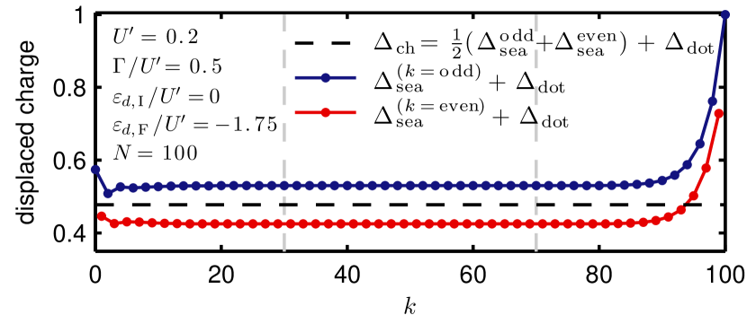
Figure 3: (Color online) Determination of $\Delta_{\mathrm{ch}}$, for the interacting resonant level model of Eq. (14), for a single specific set of parameters for ${\hat{H}_{\rm I}}$ and ${\hat{H}_{\rm F}}$, specified in the figure legend (the $\varepsilon_{{\mathrm{d}},{\rm F}}$-dependence of $\Delta_{\mathrm{AO}}$ for fixed $\varepsilon_{{\mathrm{d}},{\rm I}}$ is analyzed in more detail in Fig. 4. We obtain $\Delta_{\mathrm{ch}}$ (dashed line) by calculating $\Delta_{\mathrm{sea}}^{(k)}+{\Delta_{\mathrm{dot}}}$ and averaging the results for even and odd $k$. To reduce the influence of chain’s boundary regions, we take the average over the region between the vertical dashed lines.

IV Results

In this section, we present results for the single channel interacting resonant level model [Eq. (14)], and for single-lead and two-lead Anderson impurity models [Eq. (13)]. These examples were chosen to illustrate that the various ways of calculating AO exponents by NRG, via $\Delta_{\mathrm{AO}}$, $\Delta_{\mathrm{ph}}$ or $\Delta_{\mathrm{ch}}$, are mutually consistent with high accuracy, even for rather complex (multi-level, multi-lead) models with local interactions. In all cases, the initial and final Hamiltonians, ${\hat{H}_{\rm I}}$ and ${\hat{H}_{\rm F}}$, differ only in the level position: $\varepsilon_{d,{\rm I}}$ is kept fixed, while $\varepsilon_{d,{\rm F}}$ is swept over a range of values. This implies different initial and final dot occupations $n_{d\mu,{X}}=\langle G_{X}|\hat{n}_{{\mathrm{d}}\mu}|G_{X}\rangle$, and hence different local scattering potentials, causing AO.

AO exponents are obtained as described in the previous sections: we calculate the AO-measure $z_{GK}(k)$ using Eq. (2), obtaining exponentially decaying behavior (as in Fig. 1). We then extract $\alpha$ by fitting to $e^{-\alpha k}$ and determine $\Delta_{\mathrm{AO}}$ via Eq. (19). In the figures below, the resulting $\Delta_{\mathrm{AO}}^{2}$ is shown as function of $\varepsilon_{{\mathrm{d}}\mu,{\rm F}}$, together with $\Delta_{\mathrm{ch}}^{2}$, and also $\Delta_{\mathrm{ph}}^{2}$ in Fig. 4. The initial dot level position $\varepsilon_{{\mathrm{d}}\mu,{\rm I}}$ is indicated by a vertical dashed line. When $\varepsilon_{{\mathrm{d}}\mu,{\rm F}}$ crosses this line, the initial and final Hamiltonians are identical, so that all AO exponents vanish. To illustrate how the changes in $\varepsilon_{{\mathrm{d}}\mu,{\rm F}}$ affect the dot, we also plot the occupancies $n_{{\mathrm{d}}\mu,{\rm F}}$ of the dot levels.

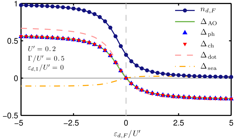
Figure 4: (Color online) Verification that $\Delta_{\mathrm{AO}}=\Delta_{\mathrm{ph}}=\Delta_{\mathrm{ch}}$ [Eq. (5)] for the spinless fermionic interacting resonant level model [Eq. 14]. All quantities are plotted as functions of $\varepsilon_{{\mathrm{d}},{\rm F}}$, with all other parameters fixed (as specified in the panel). The vertical dashed line indicates $\varepsilon_{{\mathrm{d}},{\rm I}}/U^{\prime}=0$. Heavy dots indicate the final occupation of the dot, $n_{{\mathrm{d}}}$. The exponent $\Delta_{\mathrm{AO}}$ (light solid line) agrees well with $\Delta_{\mathrm{ph}}$ and $\Delta_{\mathrm{ch}}$ (triangles), with relative errors of less than $1\%$. The local and Fermi-sea contributions to the displaced charge $\Delta_{\mathrm{ch}}$ are plotted separately, namely ${\Delta_{\mathrm{dot}}}$ (dashed line) and ${\Delta_{\mathrm{sea}}}$ (dashed dotted). The latter is determined according to the procedure illustrated, for $\varepsilon_{d,{\rm F}}/U^{\prime}=-1.75$, in Fig. 3.

IV.1 Interacting resonant-level model

We begin with a model for which the contribution of the Fermi sea to the displaced charge is rather important, namely the spinless fermionic interacting resonant level model [Eq. (14), ${N_{\mathrm{c}}}=1$]. The initial and final Hamiltonians, ${\hat{H}_{\rm I}}^{\textrm{IRLM}}$ and ${\hat{H}_{\rm F}}^{\textrm{IRLM}}$, differ only in the level position: the initial one is kept fixed at $\varepsilon_{d,{\rm I}}=0$, while the final one is swept over a range of values, $\varepsilon_{d,{\rm F}}\in[-1,1]$. The results are shown in Fig. 4. The final dot occupancy $n_{{\mathrm{d}},{\rm F}}$ (heavy dots) varies from $\simeq 1$ to $\simeq 0$, and ${\Delta_{\mathrm{dot}}}=n_{{\mathrm{d}},{\rm F}}-n_{{\mathrm{d}},{\rm I}}$ (dashed line) decreases accordingly, too. The total displaced charge, $\Delta_{\mathrm{ch}}={\Delta_{\mathrm{dot}}}+{\Delta_{\mathrm{sea}}}$ (downward-pointing triangles), decreases by a smaller amount, since the depletion of the dot implies a reduction in the strength of the local Coulomb repulsion felt by the Fermi sea, and hence an increase in ${\Delta_{\mathrm{sea}}}$ (dash-dotted line). Throughout these changes $\Delta_{\mathrm{AO}}$, $\Delta_{\mathrm{ph}}$ and $\Delta_{\mathrm{ch}}$ mutually agree with errors of less than $1\%$, confirming that NRG results comply with Eq. (5) to high accuracy.

IV.2 Single-impurity Anderson model

Next we consider the standard spin-degenerate SIAM for a single lead [Eq. (13), $\mu\in\{\uparrow,\downarrow\}$] with $\varepsilon_{{\mathrm{d}},\mu}=\varepsilon_{{\mathrm{d}}}$ and $\Gamma_{\mu}=\Gamma$. This model exhibits well-known Kondo physics, with a strongly correlated many-body ground state.

In this model, the dot and Fermi sea affect each other only by hopping, and there is no direct Coulomb interaction between them ($U^{\prime}=0$). Hence, the contribution of the Fermi sea to the displaced charge is nearly zero, ${\Delta_{\mathrm{sea}}}\simeq 0$. Apart from very small even-odd variations for the first $\sim 35$ bath sites corresponding to the Kondo scale, the sites of the Wilson chain are half-filled on average to a good approximation. Therefore ${\Delta_{\mathrm{sea}}}\ll{\Delta_{\mathrm{dot}}}$ (explicit numbers are specified in the figure panels; see also Fig. 1), so that $\Delta_{\mathrm{ch}}{}_{,\mu}$ in Eq. (7) is dominated by the change of dot occupation only, Langreth (1966)

$$\Delta_{\mathrm{ch}}^{2}\simeq\Delta_{\mathrm{dot}}^{2}\equiv\sum_{\mu}(n_{{\mathrm{d}}\mu,{\rm F}}-n_{{\mathrm{d}}\mu,{\rm I}})^{2}\text{.}$$ (27)

As a consequence, despite the neglect of ${\Delta_{\mathrm{sea}}}$ in some previous works involving Anderson impurity models, the Friedel sum rule ($\Delta_{\mathrm{ph}}=\Delta_{\mathrm{ch}}$) was nevertheless satisfied with rather good accuracy (typically with errors of a few %). However, despite being small, ${\Delta_{\mathrm{sea}}}$ in practice is on the order of $|{\Delta_{\mathrm{sea}}}|\leq\Gamma/D$ and thus finite. Therefore the contribution of ${\Delta_{\mathrm{sea}}}$ to $\Delta_{\mathrm{ch}}$ will be included throughout, while also indicating the overall smallness of ${\Delta_{\mathrm{sea}}}$. In general, this clearly improves the accuracy of the consistency checks in Eq. (5), reducing the relative errors to well below 1%.

The Anderson orthogonality is analyzed for the SIAM in detail in Fig. 5. The initial system is kept fixed at the particle-hole symmetric point, $\varepsilon_{{\mathrm{d}},{\rm I}}=-U/2$ (indicated also by vertical dashed line in panel a), where the initial ground state is a Kondo singlet. The final system is swept from double to zero occupancy by varying $\varepsilon_{{\mathrm{d}},{\rm F}}/U$ from $-2$ to 1. The final ground state is a Kondo singlet in the regime $n_{{\mathrm{d}}\mu,{\rm F}}\simeq 1/2$, corresponding to the intermediate shoulder in panel (a). Panel (b) shows the AO-measure $z_{GK}(k)$ as function of $k$, for a range of different values of $\varepsilon_{{\mathrm{d}},{\rm F}}$. Each curve exhibits clear exponential decay for large $k$ (as in Fig. 1), of the form $e^{\lambda-\alpha k}$. The prefactor, parameterized by $\lambda$, carries little physical significance, as it also depends on the specific choice of $z_{PP^{\prime}}$; its dependence on $\varepsilon_{{\mathrm{d}},{\rm F}}$ is shown as thick gray dashed line in panel (a), but it will not be discussed any further. In contrast, the decay exponent $\alpha$ directly yields the quantity of physical interest, namely the AO exponent $\Delta_{\mathrm{AO}}^{2}$ via Eq. (19). Panel (a) compares the dependence on $\varepsilon_{{\mathrm{d}},{\rm F}}$ of $\Delta_{\mathrm{AO}}^{2}$ (dashed line) with that of the displaced charge $\Delta_{\mathrm{ch}}^{2}$ (light thick line), that was calculated independently from Eqs. (7) and (8). As expected from Eq. (5), they agree very well: the relative difference between the two exponents $\Delta_{\mathrm{AO}}^{2}$ and $\Delta_{\mathrm{ch}}^{2}$ is clearly below $1\%$ throughout the entire parameter sweep, as shown in the inset of Fig. 5(b).

The contribution of the Fermi sea to the displaced charge is close to negligible, yet finite throughout (black line in panel a). Overall, ${\Delta_{\mathrm{sea}}}\lesssim 0.0037$, as indicated in Eq. (27). Nevertheless, by including it when calculating $\Delta_{\mathrm{ch}}$, the relative error $\delta\Delta^{2}$ is systematically reduced from a few percent to well below 1% throughout, thus underlining its importance.

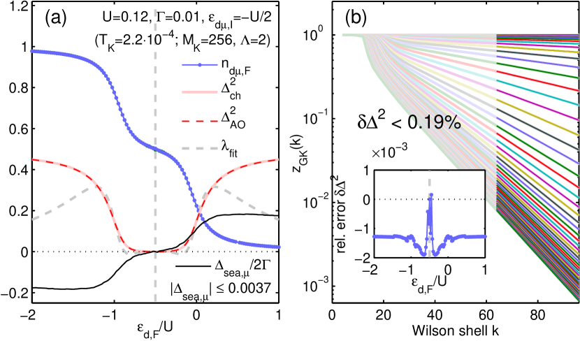
Figure 5: (Color online) Anderson orthogonality for the single-lead, spin-symmetric SIAM [Eq. (13), with parameters as specified in the legend] – The energy of the $d$-level of the final system $\varepsilon_{{\mathrm{d}},{\rm F}}$ is swept past the Fermi energy of the bath, while that of the initial reference system is kept fixed in the Kondo regime at $\varepsilon_{{\mathrm{d}},{\rm I}}=-U/2$, indicated by vertical dashed line in panel (a) and in inset to panel (b). Panel (a) shows, as function of $\varepsilon_{{\mathrm{d}},{\rm F}}$, the dot occupation per spin $n_{{\mathrm{d}}\mu}$ (dotted solid line), the contribution to the displaced charge by the Fermi sea, ${\Delta_{\mathrm{sea}}}_{\mu}$ (thin black line), the displaced charge $\Delta_{\mathrm{ch}}^{2}$ (light solid line), and the parameters of the large-$k$ exponential decay $e^{\lambda-\alpha k}$ of $z_{GK}(k)$ as extracted from panel (b), namely $\lambda$ (thick dashed line) and $\Delta_{\mathrm{AO}}$ (dark dashed line), derived from $\alpha$ via Eq. (19). Panel (b) shows the AO-measure $z_{GK}(k)$ in Eq. (2) (light lines) for the range of $\varepsilon_{{\mathrm{d}},{\rm F}}$ values used in panel (a). The heavy lines shown on top for $k\geq 64$ are exponential fits, the results of which are summarized in panel (a). The inset shows the relative error in the AO exponents $\delta\Delta^{2}\equiv(\Delta_{\mathrm{AO}}^{2}-\Delta_{\mathrm{ch}}^{2})/\Delta_{\mathrm{ch}}^{2}$, i.e. the deviation between the light solid and dark dashed curve in panel (a); this error is clearly less than $1\%$ over the full range of $\varepsilon_{{\mathrm{d}}}$ analyzed.

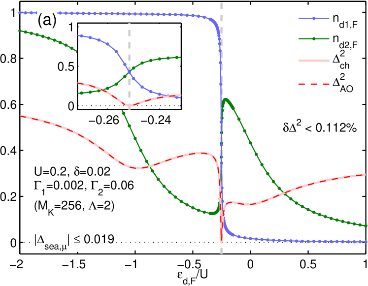
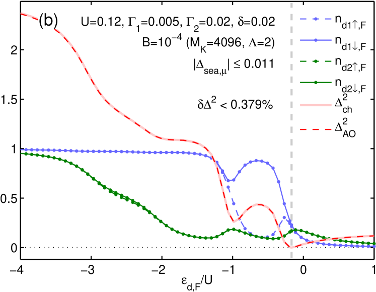
Figure 6: (Color online) Anderson orthogonality for a spinless (panel a) and spin-full (panel b) two-lead SIAM, with dot levels of unequal width and a split level structure as defined in Eq. (28) (all relevant model parameters are specified in the legends) – In both cases, the higher level 2 is broader than the lower level 1 $(\Gamma_{2}>\Gamma_{1})$, leading to population switching as function of the average final level energy $\varepsilon_{{\mathrm{d}},{\rm F}}$. The fixed value of $\varepsilon_{{\mathrm{d}},{\rm I}}$ is indicated by the vertical dashed line. The inset to panel (a) shows a zoom into the switching region, clearly demonstrating that population switching occurs smoothly. For panel (b), a finite magnetic field $B$ causes a splitting between spin-up and spin-down levels, resulting in a more complex switching pattern. In both panels $\Delta_{\mathrm{AO}}^{2}$ and $\Delta_{\mathrm{ch}}$ agree very well throughout the sweep, with a relative error $\delta\Delta^{2}$ well below $1\%$.

IV.3 Multiple Channels and Population switching

Figure 6 analyzes AO for lead-asymmetric two-level, two-lead SIAM models, with Hamiltonians of the form Eq. (13) (explicit model parameters are specified in the panels). Panel (a) considers a spinless case (${N_{\mathrm{c}}}=2$, $\mu=j\in\{1,2\}$), whose dot levels have mean energy $\varepsilon_{{\mathrm{d}}}$ at fixed splitting $\delta$,

$$\varepsilon_{{\mathrm{d}}1}=\varepsilon_{{\mathrm{d}}}-\delta/2,\quad\varepsilon_{{\mathrm{d}}2}=\varepsilon_{{\mathrm{d}}}+\delta/2.$$ (28a)

Panel (b) considers a spinfull case, ($${N_{\mathrm{c}}}=4 \mu=(j\sigma) j\in\{1,2\} \sigma\in\{\uparrow,\downarrow\} B\ll\delta$$, with , ), where both the lower and upper levels have an additional (small) spin splitting ,

$$\varepsilon_{{\mathrm{d}}j\uparrow}=\varepsilon_{{\mathrm{d}}j}+B/2,\quad\varepsilon_{{\mathrm{d}}j\uparrow}=\varepsilon_{{\mathrm{d}}j}-B/2\;.$$ (28b)

Charge is conserved in each of the ${N_{\mathrm{c}}}$ channels, since these only interact through the interaction on the dot. In both models, the upper level 2 is taken to be broader than the lower level 1, $\Gamma_{2}>\Gamma_{1}$ (for detailed parameters, see figure legends). As a consequence, Silvestrov and Imry (2000); Golosov and Gefen (2006); Karrasch et al. (2007); Goldstein et al. (2010) these models exhibit population switching: when $\varepsilon_{{\mathrm{d}},{\rm F}}$ is lowered (while all other parameters are kept fixed), the final state occupancies of upper and lower levels cross, as seen in both panels of Fig. 6.

Consider first the spinless case in Figure 6(a). The broader level 2 shows larger occupancy for large positive $\varepsilon_{{\mathrm{d}},{\rm F}}$. However, once the narrower level 1 drops sufficiently far below the Fermi energy of the bath as $\varepsilon_{{\mathrm{d}},{\rm F}}$ is lowered, it becomes energetically favorable to fill level 1, while the Coulomb interaction will cause the level 2 to be emptied. At the switching point, occupations can change extremely fast, yet they do so smoothly, as shown in the zoom in the inset to panel (a).

Similar behaviour is seen for the spinfull case in Figure 6(b), though the filling pattern is more complex, due to the nonzero applied finite magnetic field $B$ (parameters are listed in the legend). The occupations $n_{{\mathrm{d}}1\sigma}$ of the narrower level 1 show a strong spin asymmetry, since the magnetic field is comparable, in order of magnitude, to the level width ($B=\Gamma_{1}/2$). This asymmetry affects the broader level 2, which fills more slowly as $\varepsilon_{d}$ is lowered. Due to the larger width of level 2, the asymmetry in its spin-dependent occupancies is significantly weaker. As in panel (a), population switching between the two levels occurs: as the narrower level 1 becomes filled, the broader level 2 gets depleted.

The details of population switching, complicated as they are (extremely rapid in panel (a); involving four channels in panel (b)), are not main point of Fig. 6. Instead, its central message is that despite the complexity of the switching pattern, the relation $\Delta_{\mathrm{AO}}^{2}=\Delta_{\mathrm{ch}}^{2}$ is satisfied with great accuracy throughout the sweep (compare light thick and dark dashed lines). Moreover, since $\Delta_{\mathrm{ch}}$ was calculated by adding the contributions from separate channels according to Eq. (8), this also confirms the additive character of AO exponents for separate channels.

As was the case for the single-channel SIAM discussed in Sec. IV.2 above, a direct interaction between dot and Fermi sea is not present in either of the models considered here $(U^{\prime}=0)$. Consequently, the displaced charge $\Delta_{\mathrm{ch}}$ is again dominated by ${\Delta_{\mathrm{dot}}}$, with ${\Delta_{\mathrm{sea}}}\ll{\Delta_{\mathrm{dot}}}$ (cf. Eq. 27). Specifically, for the spinless or spinfull models, we find ${\Delta_{\mathrm{sea}}}<0.019$ or $0.011$, respectively, for the entire sweep.

V Summary and Outlook

In summary, we have shown that NRG offers a straightforward, systematic and self-contained way for studying Anderson orthogonality, and illustrated this for several interacting quantum impurity models. The central idea of our work is to exploit the fact that NRG allows the size-dependence of an impurity model to be studied, in the thermodynamic limit of $N\to\infty$, by simply studying the dependence on Wilson chain length $k$. Three different ways of calculating AO exponents have been explored, using wave-function overlaps ($\Delta_{\mathrm{AO}}$), changes in phase shift at the Fermi surface ($\Delta_{\mathrm{ph}}$), and changes in displaced charge ($\Delta_{\mathrm{ch}}$). The main novelty in this paper lies in the first of these, involving a direct calculation of the overlap of the initial and final ground states themselves. This offers a straightforward and convenient way for extracting the overall exponent $\Delta_{\mathrm{AO}}$. Moreover, if desired, it can also be used to calculate the exponents ${\Delta_{\mathrm{AO}}}_{,\mu}$ associated with individual channels, by constructing a Wilson chain that is longer for channel $\mu$ than for the others. We have also refined the calculation of $\Delta_{\mathrm{ch}}$, by showing how the contribution ${\Delta_{\mathrm{sea}}}$ of the Fermi sea to the displaced charge can be taken into account in a systematic fashion.

The resulting exponents $\Delta_{\mathrm{AO}}$, $\Delta_{\mathrm{ph}}$ and $\Delta_{\mathrm{ch}}$ agree extraordinarily well, with relative errors of less than 1%. This can be achieved using a remarkably small number of kept states $M_{K}$. For example, for the spinfull SIAM analyzed below, a better than 5% agreement can be obtained already for $M_{K}\geq 32$. (For comparison, typically $M_{K}=250$ is required to obtain an accurate description of the Kondo resonance of the $d$-level spectral function in the local moment regime of this model.)

Our analysis has been performed on models exhibiting Fermi liquid statistics at low temperatures. As an outlook, it would be interesting to explore to what extent the non-Fermi liquid nature of a model would change AO scaling properties, an example being the symmetric spinful two-channel Kondo model.

Finally, we note that non-equilibrium simulations of quantum impurity models in the time-domain in response to quantum quenches are a highly interesting topic for studying AO physics in the time domain. The tools to do so using NRG have become accessible only rather recently. Anders and Schiller (2005, 2006); Weichselbaum and von Delft (2007); Türeci et al. (2009) One considers a sudden change in some local term in the Hamiltonian and studies the subsequent time-evolution, characterized, for example, by the quantity $\langle G_{\rm I}|e^{-i{\hat{H}_{\rm F}}t}|G_{\rm I}\rangle$. Its numerical evaluation requires the calculation of overlaps of eigenstates of ${\hat{H}_{\rm I}}$ and ${\hat{H}_{\rm F}}$. The quantity of present interest, $|\langle G_{\rm I}|G_{\rm F}\rangle|$, is simply a particular example of such an overlap. As a consequence, the long-time decay of $\langle G_{\rm I}|e^{-i{\hat{H}_{\rm F}}t}|G_{\rm I}\rangle$ is often governed by $\Delta_{\mathrm{AO}}$, too, Nozières et al. (1969); Schotte and Schotte (1969b) showing power-law decay in time with an exponent depending on $\Delta_{\mathrm{AO}}$. This will be elaborated in a separate publication.Muender2011b

- (1)
- Anderson (1967) P. W. Anderson, Phys. Rev. Lett. 18, 1049 (1967).
- Mahan (1967) G. D. Mahan, Phys. Rev. 153, 882 (1967).
- Schotte and Schotte (1969b) K. D. Schotte and U. Schotte, Phys. Rev. 182, 479 (1969b).
- Schotte and Schotte (1969a) K. D. Schotte and U. Schotte, Phys. Rev. 185, 509 (1969a).
- Nozières et al. (1969) P. Nozières, J. Gavoret, and B. Roulet, Phys. Rev. 178, 1084 (1969).
- Yuval and Anderson (1970) G. Yuval and P. W. Anderson, Phys. Rev. B 1, 1522 (1970).
- Kondo (1964) J. Kondo, Prog. Theor. Phys. 32, 37 (1964).
- Goldhaber-Gordon et al. (1998) D. Goldhaber-Gordon, J. Göres, M. A. Kastner, H. Shtrikman, D. Mahalu, and U. Meirav, Phys. Rev. Lett. 81, 5225 (1998).
- Helmes et al. (2005) R. W. Helmes, M. Sindel, L. Borda, and J. von Delft, Phys. Rev. B 72, 125301 (2005).
- Türeci et al. (2009) H. E. Türeci, M. Hanl, M. Claassen, A. Weichselbaum, T. Hecht, B. Braunecker, A. Govorov, L. Glazman, J. von Delft, and A. Imamoglu, Phys. Rev. Lett. 106, 107402 (2011).
- Latta et al. (2009) C. Latta, F. Haupt, M. Hanl, A. Weichselbaum, M. Claassen, W. Wuester, P. Fallahi, S. Faelt, L. Glazman, J. von Delft, H. E. Türeci, and A. Imamoglu, arXiv:1102.3982v1 [cond-mat.mes-hall] (2011).
- (13) W. Münder, A. Weichselbaum, M. Goldstein, Y. Gefen, and J. von Delft, in preparation (2011).
- Wilson (1975) K. G. Wilson, Rev. Mod. Phys. 47, 773 (1975).
- Bulla et al. (2008) R. Bulla, T. A. Costi, and T. Pruschke, Rev. Mod. Phys. 80, 395 (2008).
- Anders and Schiller (2005) F. B. Anders and A. Schiller, Phys. Rev. Lett. 95, 196801 (2005).
- Anders and Schiller (2006) F. B. Anders and A. Schiller, Phys. Rev. B 74, 245113 (2006).
- Weichselbaum and von Delft (2007) A. Weichselbaum and J. von Delft, Phys. Rev. Lett. 99, 076402 (2007).
- Weichselbaum et al. (2009) A. Weichselbaum, F. Verstraete, U. Schollwock, J. I. Cirac, and J. von Delft, Phys. Rev. B. 80, 165117 (2009).
- Schollwöck (2011) U. Schollwöck, Ann. Phys. 326, 96 (2011).
- Silvestrov and Imry (2000) P. Silvestrov and Y. Imry, Phys. Rev. Lett. 85, 2565 (2000).
- Golosov and Gefen (2006) D. I. Golosov and Y. Gefen, Phys. Rev. B 74, 205316 (2006).
- Karrasch et al. (2007) C. Karrasch, T. Hecht, A. Weichselbaum, Y. Oreg, J. von Delft, and V. Meden, Phys. Rev. Lett. 98, 186802 (2007).
- Goldstein et al. (2010) M. Goldstein, R. Berkovits, and Y. Gefen, Phys. Rev. Lett. 104, 226805 (2010).
- Friedel (1956) J. Friedel, Can. J. Phys. 34, 1190 (1956).
- Langreth (1966) D. C. Langreth, Phys. Rev. 150, 516 (1966).