Re-assigning (1$\times$2) reconstruction of rutile TiO₂(110) from DFT+U calculations

Abstract

Physically reasonable electronic structures of reconstructed rutile TiO₂(110)-(1$\times$2) surfaces were studied using density functional theory (DFT) supplemented with Hubbard $U$ on-site Coulomb repulsion acting on the $d$ electrons, so called as the DFT+$U$ approach. Two leading reconstruction models proposed by Onishi–Iwasawa and Park et al. were compared in terms of their thermodynamic stabilities.

Rutile TiO₂ and its surfaces represent model systems to explore the properties of transition metal oxides that are important in technological applications such as catalysis, photovoltaics, and gas sensing diebold1 , to name a few. Truncated or stoichiometric (110) surface of rutile is the most stable one among all surfaces of titania heinrich . Upon thermal annealing or ion bombardment TiO₂(110)-(1$\times$1) surface is reduced by loosing the bridging oxygens, and is often undergo a (1$\times$2) reconstruction with row formations onishi ; murray ; guo ; pang ; elliot1 ; elliot2 ; mccarty ; blancorey1 ; blancorey2 ; park ; shibata . The identification of these rows on reconstructed surfaces, in three dimensions, is difficult by experimental methods shibata . The best candidate for modeling this reconstruction involves the addition of “Ti₂O₃” molecule on the surface unit cell (added-row model) proposed by Onishi and Iwasawa onishi . In addition to theoretical studies it was supported by electron stimulated desorption of ion angular distribution (ESDIAD), scanning tunnelling microscopy (STM), and low-energy electron diffraction (LEED) experiments guo ; pang ; elliot1 ; elliot2 ; mccarty ; blancorey1 ; blancorey2 . On the other hand, Shibata et al. shibata , using advanced transmission electron microscopy (TEM) observations reported results that are consistent with a different model, proposed by Park et al. park , for which the additional unit is “Ti₂O”. The main difference between the Onishi–Iwasawa and Park et al. models (Onishi and Park models, respectively, in what follows) is the locations of Ti interstitial sites on the surface shibata (see Fig. 1).

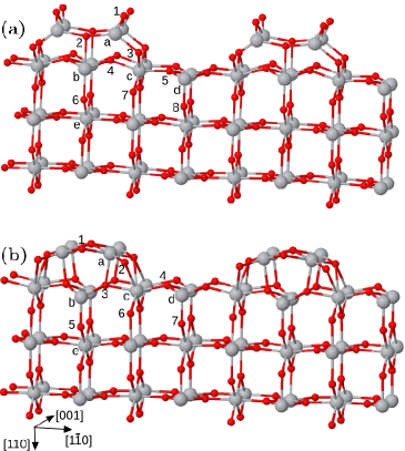
Figure 1: Fully relaxed (1$\times$2) reconstructed rutile TiO₂(110) surface models of (a) Onishi–Iwasawa onishi and (b) Park  et al. park showing 3 Ti-layers from the top.

Now there is a debate about which formation gives rise to the (1$\times$2) long range order, the last proposed one or the best previous candidate? In this context we study the electronic properties of these two models using Hubbard $U$ corrected total energy density functional theory (DFT+$U$) calculations to get physically reasonable results comparable to existing experimental data. We discuss which of these leading models can be assigned to describe the (1$\times$2) reconstructed surface by comparing them according to their thermodynamic stabilities.

Band structures of reduced and reconstructed TiO₂(110) surfaces determined by pure DFT calculations does not agree with experiments kimmel ; kruger ; blancorey1 . Failure of the standart DFT is not limited to band-gap underestimation stemming from the many-electron self-interaction error (SIE). More importantly, it does not predict experimentally observed gap states henrich ; henderson that are associated with the excess electrons due to the formation of surface oxygen vacancies. In DFT calculations, these Ti $3d$ electrons occupy the bottom of the conduction band (CB) giving metallic character. Hence, hybrid DFT methods need to be used. For instance, SIE can be partly corrected by partially mixing nonlocal Fock exchange term with DFT exchange term yfzhang ; valentin or DFT+$U$ approach dudarev can make up for the lack of strong correlation between the 3$d$ electrons, a shortcoming of common exchange–correlation functionals. Empirical Hubbard $U$ term accounts for the on-site Coulomb repulsion between the Ti $3d$ electrons. By examining different values of the $U$ parameter, experimentally observed gap state of the reduced TiO₂(110) surface was obtained $\sim$0.7–0.9 eV below the CB morgan ; calzado ; nolan .

For the (1$\times$2) reconstructed surface with Ti₂O₃ added row, Kimura et al. kimura , and then, Blanco-Rey et al. blancorey1 , obtained the Ti 3$d$ states positioned inside the CB, and proposed this model to be metallic by pure DFT methods. Recently, using spin polarized DFT+$U$ calculations with a suitable choice of the $U$ parameter, we have shown that the Onishi model can be semiconducting celik as the reconstructed surface is observed experimentally abad . Important questions still remain to be answered such as where the excess charge density is distributed and which model structure describes the (1$\times$2) reconstruction.

We used Perdew–Burke–Ernzerhof (PBE) pbe gradient corrected exchange–correlation functional supplemented with Dudarev’s $U$ term dudarev as implemented in the VASP code vasp . The ionic cores and valence electrons were treated by the projector-augmented waves (PAW) method paw1 ; paw2 up to a cutoff value of 400 eV. In order to get well converged energetics, we adopted stoichiometric slabs with 10 Ti-layers (30 atomic layers) separated by $\sim$15 Å vacuum from their periodic images. We built the Onishi and the Park models of (1$\times$2) reconstructed rutile (110) surfaces by adding Ti₂O₃ and Ti₂O groups, respectively, along [001] both at the top and at the bottom of the slabs (see Fig. 1). Hence, having an unphysical dipole across the slab and getting two different groups of surface states in the gap has been avoided. Instead, symmetric slabs bring about the same group of surface states (degenerate) from both surfaces.

Our choice of $U$=5 eV follows from our examination of the effect of different $U$ values on both the geometry and the energy bands of rutile TiO₂. While a larger $U$ value can give a wider band gap, it would make a significant distortion in the atomic structure. Inclusion of Dudarev $U$=5 eV term acting on Ti 3$d$ electrons gave reasonable values for the atomic positions with bond lengths in agreement with the experimental data for the stoichiometric, reduced, and the reconstructed rutile (110) surfaces. This choice is also consistent with the previous calculations describing the reduced morgan ; calzado ; nolan and reconstructed celik surfaces. Spin polarization was also found to be important in determining the semiconducting ground state of reconstructed surfaces and in correctly describing Ti defect states while it is insignificantly small for the stoichiometric surface. Our PBE+$U$ calculations determined the ground states with spin multiplicities of 2 and 6 per surface of (1$\times$2) unit cells for Onishi and Park models, respectively.

Table 1: PBE+$U$ results of atomic positions for the Onishi model with $U$=5 eV.

	Theoretical (Å)			Experimental (Å)
Atom	$x$ [001]	$y$ [11̄0]	$z$ [110]	$x$	$y$	$z$
Ti(a)	1.48	1.76	$-5.77$	1.48	1.77	$-5.99\pm$0.03
Ti(b)	1.48	$-0.14$	$-3.36$	1.48	0.00	$-3.14\pm$0.07
Ti(c)	$-0.04$	3.23	$-3.28$	0.00	3.28	$-3.27\pm$0.06
Ti(d)	1.48	6.44	$-3.03$	1.48	6.49	$-3.08\pm$0.05
O(1)	$-0.04$	2.08	$-6.81$	0.00	1.99	$-7.16\pm$0.24
O(2)	1.48	$-0.15$	$-5.53$	1.48	0.00	$-5.23\pm$0.07
O(3)	1.48	3.35	$-4.62$	1.48	3.07	$-4.60\pm$0.11
O(4)	$-0.04$	1.30	$-3.86$	0.00	1.25	$-3.21\pm$0.12
O(5)	$-0.04$	5.20	$-3.35$	0.00	5.22	$-3.54\pm$0.06
O(6)	1.48	$-0.13$	$-1.35$	1.48	0.00	$-1.30\pm$0.22
O(7)	1.48	3.09	$-2.01$	1.48	3.28	$-2.03\pm$0.22
O(8)	1.48	6.44	$-1.23$	1.48	6.49	$-1.31\pm$0.12

Table 2: PBE+$U$ results of atomic positions for the Park model with $U$=5 eV.

	Theoretical (Å)			Experimental (Å)
Atom	$x$ [001]	$y$ [11̄0]	$z$ [110]	$x$	$y$	$z$
Ti(a)	0.02	1.56	$-5.48$	0.00	1.57	$-5.12\pm$0.14
Ti(b)	1.48	0.00	$-2.80$	1.48	0.00	$-3.14\pm$0.10
Ti(c)	$-0.05$	3.34	$-3.15$	0.00	3.32	$-3.26\pm$0.10
Ti(d)	1.48	6.58	$-3.12$	1.48	6.49	$-3.52\pm$0.06
O(1)	1.65	0.00	$-5.89$	1.48	0.00	$-5.30\pm$0.12
O(2)	1.47	2.83	$-5.12$	1.48	3.14	$-4.63\pm$0.14
O(3)	$-0.04$	1.28	$-3.45$	0.00	1.26	$-3.32\pm$0.18
O(4)	$-0.04$	5.32	$-3.57$	0.00	5.22	$-3.48\pm$0.16
O(5)	1.48	0.00	$-0.90$	1.48	0.00	$-1.38\pm$0.32
O(6)	1.47	3.24	$-1.85$	1.48	3.24	$-2.04\pm$0.12
O(7)	1.48	6.58	$-1.32$	1.48	6.49	$-1.28\pm$0.20

Calculated atomic coordinates and the LEED results blancorey1 ; blancorey2 are only slightly different as shown in Table 1 and Table 2 for each of the model structures. The most noticeable deviation is seen in the $z$ component of O(4) in the Onishi model. While keeping distortion to the atomic positions small, PBE+$U$ with $U$=5 eV reproduces the gap states as shown in Fig. 2. Defect states has been found to be 1.24 eV and 0.68 eV below the CB for Onishi and Park models, respectively, in agreement with experiments henrich ; henderson . In the Onishi model, the gap state with a dispersion width of 0.65 eV reveal charge delocalization to the interstitial Ti atom just below in-plane Ti5c showing $d_{z^{2}}$ character and to the oxygen atom beneath it as shown in Fig. 3.

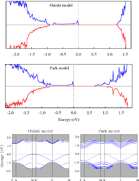
Figure 2: Density of states (DOS) plots and energy band diagrams for the majority electrons belonging to Onishi onishi and Park park models of TiO₂(110)-(1$\times$2) surface.

As finding the almost correct position of the experimentally observed Ti $3d$ states, describing the origin of those states is also important. According to the ultraviolet photoelectron spectroscopy (UPS) and LEED experiments, the excess electrons upon O loss are believed to delocalize around the surface Ti atoms, adjacent to the vacancies henrich . Although this vacancy model is supported by some calculations valentin ; morgan , there are studies that indicate the role of subsurface Ti atoms about the delocalization of the excess charge onishi ; bennet2 ; wendt . Since pure DFT gives a clean band gap, based on their STM and UPS measurements Wendt et al. proposed that the gap states originate from Ti atoms diffused into interstitial sites, not from the surface Ti atoms adjacent to bridging O vacancies wendt . Without a need to such an additional interstitial Ti atom, delocalization of the excess charge to the subsurface Ti, responsible for the gap state, emerges from DFT+$U$ calculations as shown in Fig. 3.

Surface free energy is a good measure to compare the thermodynamic stability of model row formations. Stoichiometric cell is a stack of Ti₄O₈-(1$\times$2) units that act as bulk layers around the central regions as taken into account in Ref. elliot2 . Our ten Ti-layer slab model can be expressed as Ti_nO_2n with $n=40$. Reduced reconstructions are led by surface O removal from the stoichiometric surface. For our symmetrical slab cell, Ti_nO_2n-m represents both the Onishi ($m$=2) and the Park ($m$=6) models. Then, the surface energies were calculated by the relation,

$$\sigma=\frac{1}{2A}\;(E_{n}^{\rm slab}-nE^{\rm bulk}+mE^{\rm O})\,,$$

where $A$ is the surface unit cell area, $E_{n}^{\rm slab}$, $E^{\rm bulk}$, and $E^{\rm O}$ are the energies of a Ti_nO_2n-m slab, of a bulk Ti₄O₈ unit ($-89.3$ eV) and of an oxygen atom in its molecular form, respectively. Division by two is because the slab has two reconstructed surfaces on its both faces. In an experiment, the surface layer is an interface between O₂ gas phase and TiO₂ bulk crystal. Thermal equilibrium can exist if the chemical potential of the atomic species are equal in all these phases that come into contact with each other. Therefore, determination of the chemical potential of oxygen atom, $E^{\rm O}$, limits the accuracy of the calculated surface energies. We found the binding energy of an O₂ molecule to be 6.07 eV which is significantly larger than the experimental value of 5.26 eV nist . The tendency of DFT to overestimate it, was also reported previously morgan ; kowalski . Therefore, in order to obtain a more reasonable energy value for $E^{\rm O}$, we adopted the experimental binding energy of O₂ (5.26 eV) and DFT result of an isolated O atom ($-1.89$ eV). It gives $-4.52$ eV for $E^{\rm O}$. By using this reference chemical potential we calculated the formation energy of bulk TiO₂ from metallic bulk Ti and O₂ molecule as 9.72 eV, in excellent agreement with the experimental value of 9.73 eV nist . Therefore thermodynamic equilibrium between the surface and the bulk crystal can also be reached.

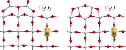
Figure 3: Partial charge densities of the gap states.

In Fig. 4 we compare relative stabilities of stoichiometric and reconstructed slabs through their surface energies with varying number of Ti-layers. Surface energetics of the stoichiometric slab at the Hartree–Fock and at the standard DFT levels were reported to exhibit odd–even oscillations with the number of layers bates ; kiejna ; labat ; kowalski . Our results show that the oscillation of both the stoichiometric and reduced surface energies with slab thickness settles down by the inclusion of $U$=5 (Fig. 4). Using ten Ti-layer cells we calculated well converged surface free energies as 0.74, 2.03, and 4.82 J$\cdot$m^-2, for the stoichiometric and reconstructed (Onishi and Park models) surfaces, respectively. Our results are significantly different from the calculations carried out with pure functionals. For instance, Morgan et al. calculated the surface energy of stoichiometric case to be 0.58 J$\cdot$m^-2 using GGA and to be 0.83 J$\cdot$m^-2 using GGA+$U$ ($U$=4.2 eV) over (4$\times$2) supercell with five Ti-layers morgan . The latter is in good agreement with our GGA+$U$ value of 0.86 J$\cdot$m^-2 calculated with 5-Ti-layer stoichiometric (1$\times$2) supercell. For the Ti₂O₃ added row model, Elliot et al. found the surface energy using spin-polarized DFT to be 3.29$\pm$0.08 J$\cdot$m^-2 which is corrected by the absolute energy value of an isolated oxygen atom elliot1 . On the other hand, for recent Ti₂O model of Park et al., no calculations for the surface energy were reported.

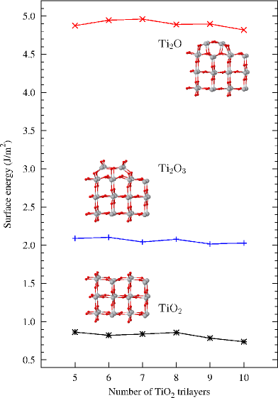
Figure 4: Calculated free energies of TiO₂(110) surface models.

Relaxed bulk termination appears to be the most stable surface. Once the TiO₂(110) surface is reduced (followed by a reconstruction), O₂ exposure can not restore the stoichiometric form again wendt . Thus, comparison between the reconstruction models is more meaningful. Formation energy of the Ti₂O₃ added row proposed by Onishi and Iwasawa (with a ground state spin polarization of $\mu=2$) is only 1.29 J$\cdot$m^-2 higher relative to that of the stoichiometric surface.

Standard DFT incorrectly predicts Ti $3d$ excess charge to occupy the bottom of the CB leading to metallization for the reduced and reconstructed surfaces. PBE+$U$ method with $U$=5 reproduces experimentally observed gap states for the (1$\times$2) reconstructions as well as for the oxygen vacancies on the rutile (110) surfaces. Finally, inclusion of a suitably chosen $U$ parameter in the calculations for the reconstructed rutile TiO₂(110) surface, is a simple and promising way of restoring its semiconducting nature by reproducing the band-gap states which arise from delocalization of Ti $3d$ excess charge to subsurface Ti sites. According to their surface energies, Onishi’s added row model is more stable than the Park model. Therefore, Ti₂O₃ added row model confirms existing experimental observations and can still be assigned as the (1$\times$2) long range order on the rutile (110) surface.

- (1) U. Diebold, Surf. Sci. Rep. 48, 53 (2003).
- (2) V. E. Heinrich, P. A. Cox, The Surface Science of Metal Oxides, (Cambridge Univ. Press, Cambridge, 1994).
- (3) H. Onishi, Y. Iwasawa, Surf. Sci. Lett. 313, 783 (1994).
- (4) P. W. Murray, N. G. Condon, and G. Thornton, Phys. Rev. B 51, 10 989 (1995).
- (5) Q. Guo, I. Cocks, and E. M. Williams, Phys. Rev. Lett. 77, 3851 (1996).
- (6) C. L. Pang et al., Phys. Rev. B 58, 1586 (1998).
- (7) S. D. Elliott, S. P. Bates, Phys. Rev. B 65, 245415 (2002).
- (8) S. D. Elliott, S. P. Bates, Phys. Rev. B 67, 035421 (2003).
- (9) K. F. McCarty and N. C. Bartelt, Phys. Rev. Lett. 90, 046104 (2003).
- (10) M. Blanco-Rey et al., Phys. Rev. Lett. 96, 055502 (2006).
- (11) M. Blanco-Rey et al., Phys. Rev. B 75, 081402(R) (2007).
- (12) K. T. Park, M. Pan, V. Meunier, and E. W. Plummer, Phys. Rev. B 75, 245415 (2007).
- (13) N. Shibata et al., Science 322,570 (2008).
- (14) G. A. Kimmel and N. G. Petrik, Phys. Rev. Lett. 100, 196100 (2008).
- (15) P. Kruger et al., Phys. Rev. Lett. 100, 055501 (2008).
- (16) M. A. Henderson et al., J. Phys. Chem. B 107, 534 (2007).
- (17) V. E. Henrich, G. Dresselhaus, and H. J. Zeiger, Phys. Rev. Lett. 36, 1335 (1976).
- (18) Y.-F. Zhang et al., J. Phys. Chem. B 109, 19270 (2005).
- (19) C. Di Valentin et al., Phys. Rev. Lett. 97, 166803 (2006).
- (20) S. L. Dudarev et al., Phys. Rev. B 57, 1505 (1998).
- (21) B. J. Morgan, G. W. Watson, Surf. Sci. 601, 5034 (2007).
- (22) C. J. Calzado, N. C. Hernandez, and J. F. Sanz, Phys. Rev. B 77, 045118 (2008).
- (23) M. Nolan, S. D. Elliot, J. S. Mulley, R. A. Bennet, M. Basham, P. Mulheran, Phys. Rev. B 77, 235424 (2008).
- (24) S. Kimura and M. Tsukada, Appl. Surf. Sci. 130–132, 587 (1998).
- (25) V. Çelik et al., Phys. Rev. B 82, 205113 (2010).
- (26) J. Abad et al., Appl. Surf. Sci. 234, 497 (2004).
- (27) J. P. Perdew, K. Burke, and M. Ernzerhof, Phys. Rev. Lett. 77, 3865 (1996).
- (28) G. Kresse and J. Hafner, Phys. Rev. B, 47, 558 (1993).
- (29) P. E. Blöchl, Phys. Rev. B 50, 17953 (1994).
- (30) G. Kresse and J. Joubert, Phys. Rev. B 59, 1758 (1999).
- (31) R. A. Bennett, P. Stone, N. J. Price, and M. Bowker, Phys. Rev. Lett. 82, 3831 (1999).
- (32) S. Wendt et al., Science 320, 1755 (2008).
- (33) NIST Standard Reference Database no. 69 in NIST Chemistry WebBook, edited by P. J. Linstrom and W. G. Mallard, National Institute of Standards and Technology, Gaithersburg, MD (2001).
- (34) P. M. Kowalski, B. Meyer, and D. Marx, Phys. Rev. B 79, 115410 (2009).
- (35) S. P. Bates, G. Kresse, and M. J. Gillan, Surf. Sci. 385, 386 (1997).
- (36) A. Kiejna et al., Condens. Matter 18, 4207 (2006).
- (37) F. Labat et al., J. Chem. Theory Comput. 4, 341 (2008).