Consistency of the mean and the principal components of spatially distributed functional data

Abstract

This paper develops a framework for the estimation of the functional mean and the functional principal components when the functions form a random field. More specifically, the data we study consist of curves $X(\mathbf{s}_{k};t),t\in[0,T]$, observed at spatial points $\mathbf{s}_{1},\mathbf{s}_{2},\ldots,\mathbf{s}_{N}$. We establish conditions for the sample average (in space) of the $X(\mathbf{s}_{k})$ to be a consistent estimator of the population mean function, and for the usual empirical covariance operator to be a consistent estimator of the population covariance operator. These conditions involve an interplay of the assumptions on an appropriately defined dependence between the functions $X(\mathbf{s}_{k})$ and the assumptions on the spatial distribution of the points $\mathbf{s}_{k}$. The rates of convergence may be the same as for i.i.d. functional samples, but generally depend on the strength of dependence and appropriately quantified distances between the points $\mathbf{s}_{k}$. We also formulate conditions for the lack of consistency.

and

1 Introduction

This paper develops aspects of theory for functional data observed at spatial locations. The data consist of curves $X(\mathbf{s}_{k})=\{X(\mathbf{s}_{k};t),t\in[0,T]\}$, observed at spatial points $\mathbf{s}_{1},\mathbf{s}_{2},\ldots,\mathbf{s}_{N}$. Such data structures are quite common, but often the spatial dependence and the spatial distribution of the points $\mathbf{s}_{k}$ are not taken into account. A well-known example is the Canadian temperature and precipitation data used in Ramsay and Silverman [24]. The annual curves are available at 35 locations, some of which are quite close, and so the curves have very similar characteristics, others are very remote with notably different curves.

There has not been much research on fundamental properties of spatially distributed functional data. Delicado et al. [6] review recent contributions to the methodology for spatially distributed functional data. For geostatistical functional data, several exploratory approaches to kriging have been proposed. Typically fixed basis expansions are used, see Yamanishi and Tanaka [29] and Bel et al. [1]. A general theoretical framework has to address several problems. The first issue is the dimensionality of the index space. While in time series analysis, the process is indexed by an equispaced scalar parameter, we need here a $d$-dimensional index space. For model building this makes a big difference since the dynamics and dependence of the process have to be described in all directions, and the typical recurrence equations used in time series cannot be employed. The model building is further complicated by the fact that the index space is often continuous (geostatistical data). Rather than defining a random field $\{\xi(\mathbf{s});\mathbf{s}\in\mathbb{R}^{d}\}$ via a specific model equations, dependence conditions are imposed, in terms of the decay of the covariances or using mixing conditions. Another feature peculiar to random field theory is the design of the sampling points; the distances between them play a fundamental role. Different asymptotics hold in the presense of clusters and for sparsely distributed points. At least three types of point distributions have been considered (Cressie [5]): When the region $R_{N}$ where the points $\{\mathbf{s}_{i,N};1\leq i\leq N\}$ are sampled remains bounded, then we are in the so-called infill domain sampling case. Classical asymptotic results, like the law of large numbers or the central limit theorem will usually fail, see Lahiri [17]. The other extreme situation is described by the increasing domain sampling. Here a minimum separation between the sampling points $\{\mathbf{s}_{i,N}\}\in R_{N}$ for all $i$ and $N$ is required. This is of course only possible if $\operatorname{diam}(R_{N})\to\infty$. We shall also explore the nearly infill situation studied by Lahiri [18] and Park et al. [21]. In this case, the domain of the sampling region becomes unbounded ($\operatorname{diam}(R_{N})\to\infty$), but at the same time the number of sites in any given subregion tends to infinity, that is, the points become more dense. These issues are also studied by Zhang [30], Loh [20], Lahiri and Zhu [19], Du et al. [7]. We formalize these concepts in Section 2. Finally, the interplay of the geostatistical spatial structure and the functional temporal structure must be cast into a workable framework.

The paper is organized as follows. Section 2 introduces the statistical setting. It also compares our conditions to those typically assumed for scalar spatial processes. In Sections 3 and 4 we establish consistency results, respectively, for the functional mean and the covariance operator. Section 5 explains, by means of general theorems and examples, when the sample principal components are not consistent. The proofs of the main results are collected in Section 6.

To make this presentation more streamlined, we have outsourced some proofs, further details and several examples. They are available as supplemental material: Hörmann and Kokoszka [14].

2 Preliminaries and assumptions

We assume $\{X(\mathbf{s}),\mathbf{s}\in\mathbb{R}^{d}\}$ is a random field taking values in $L^{2}=L^{2}([0,1])$, that is, each $X(\mathbf{s})$ is a square integrable function defined on $[0,1]$. The value of this function at $t\in[0,1]$ is denoted by $X(\mathbf{s};t)$. With the usual inner product in $L^{2}$, the norm of $X(\mathbf{s})$ is

$$\|X(\mathbf{s})\|=\biggl{\{}\int X^{2}(\mathbf{s};t)\,\mathrm{d}t\biggr{\}}^{1/2}.$$

The mean function $\mu(\mathbf{s})=\{EX(\mathbf{s};t),t\in[0,1]\}$ and the covariance operator is then defined for $x\in L^{2}$ by

$$C_{\mathbf{s},\mathbf{s}}(x)=E\bigl{[}\langle X(\mathbf{s})-\mu(\mathbf{s}),x\rangle\bigl{(}X(\mathbf{s})-\mu(\mathbf{s})\bigr{)}\bigr{]}.$$

More generally, we define the cross-covariance operators

$$C_{\mathbf{s}_{1},\mathbf{s}_{2}}(x)=E\bigl{[}\langle X(\mathbf{s}_{1})-\mu(\mathbf{s}_{1}),x\rangle\bigl{(}X(\mathbf{s}_{2})-\mu(\mathbf{s}_{2})\bigr{)}\bigr{]}.$$

For the existence of $C_{\mathbf{s}_{1},\mathbf{s}_{2}}$ a minimal assumption is that the variables have finite second moments in the sense that

$$E\|X(\mathbf{s})\|^{2}<\infty\qquad\forall\mathbf{s}.$$ (1)

To think of our observations $X(\mathbf{s})$ as curves in $L^{2}$ is convenient and motivated this work, but our propositions in Sections 3, 4 and 5 only require the general assumption that $\{X(\mathbf{s}),\mathbf{s}\in\mathbb{R}^{d}\}$ is a field taking values in some separable Hilbert space. So particularly our results hold true when $L^{2}$ is replaced by $\mathbb{R}^{p}$. To to the best of our knowledge, our results are new as well in the vector case.

Our goal is to estimate the unknown mean curves and the principal components (FPC’s). FPC’s are intimately connected with covariance operators, as we will describe in some detail in the next section, and likewise estimation of FPC’s is based on estimation of covariance operators. Thereby, we are estimating across space and not across time. A minimal requirement for this to make sense is then that all locations share a common mean curve and that the covariance operator is the same for all locations, respectively:

$$\mu(\mathbf{s})=\mu\quad\mbox{and}\quad C_{\mathbf{s},\mathbf{s}}=C.$$ (2)

Although (2) is apparently necessary and would also be quite natural if we were in time series context, it may be not realistic in some spatial data situations. Let us briefly sketch how our methods can still be useful by employing a spatio-temporal framework. In this case we suppose to have for each location $\mathbf{s}$ a functional time series $\{X_{i}(\mathbf{s}),i=1,2,\ldots\}$. To avoid confusion between the time parameter $i$ ($i=1,2,3,\ldots$) and the “intraday time” parameter $t$ ($t\in[0,1]$), we will employ for this paragraph the notation $X_{i}(\mathbf{s};t)$. We then assume the following model

$$X_{i}(\mathbf{s};t)=\alpha(\mathbf{s};t)+\mu_{i}(t)+Y_{i}(\mathbf{s};t),\qquad i=1,2,3,\ldots,$$

where $\{Y_{i}(\mathbf{s};t),t\in[0,1]\}$ are curves at spatial locations which satisfy (2) with $\mu\equiv 0$ and where for each fixed $\mathbf{s}$ the functional time series $\{X_{i}(\mathbf{s};\cdot),i=1,2,3,\ldots\}$ is stationary and weakly dependent (e.g., as assumed in Hörmann and Kokoszka [13]). The random curves $\{\mu_{i}(t),t\in[0,1]\}$ are zero mean curves and form a certain “basis level” shared by all curves $\{X_{i}(\mathbf{s};t),t\in[0,1]\}$ across space at time $i$. In our setup, the problem of interest is to determine for a given day $i$ the curve $\{\mu_{i}(t),t\in[0,1]\}$. We might think of daily temperature curves measured across some region. The curve $\{\mu_{i}(t),t\in[0,1]\}$ amounts to a general deviation from normal on day $i$ which persists over the whole region (e.g., on a hot day, it is not unlikely that all stations will show curves above average). Due to geographical differences the mean curves $\alpha(\mathbf{s};t)$ might be different at different locations, but they can be estimated individually by $\hat{\alpha}(\mathbf{s};t)=\frac{1}{M}\sum_{i=1}^{M}X_{i}(\mathbf{s};t)$, when we have a sample of $M$ days. So we can assume that we can detrended our data and then work with new observations $X_{i}^{\prime}(\mathbf{s};t)=\mu_{i}(t)+Y_{i}(\mathbf{s};t)$, to which our theory applies, when now $i$ is fixed.

Besides (2), we don’t impose any further stationarity assumption on the field $\{X(\mathbf{s})\}$.

2.1 Functional principal components

Functional principal components play a fundamental role in functional data analysis, much greater than the usual multivariate principal components. This is mostly due to the fact that the Karhunen–Loève expansion allows to represent functional data in a concise way. This property has been extensively used and studied in various settings. To name only a few illustrative references, we cite Hall and Hosseini-Nasab [12], Reiss and Ogden [25], Gabrys and Kokoszka [10], Benko et al. [2], Paul and Peng [22], Jiang and Wang [16] and Gabrys et al. [9]. Depending on the structure of the data, theoretical analyses emphasize various aspects of the estimation process, with smoothing in i.i.d. samples having being particularly carefully studied. This paper focuses on the spatial dependence and distribution of the curves, which has received no attention so far.

Suppose $X_{1},X_{2},\ldots,X_{N}$ are mean zero identically distributed elements of $L^{2}$ such that $E\|X\|^{4}<\infty$. The eigenfunctions of the covariance operator of $X_{1}$ are the functional principal components, denoted $v_{k}$. Up to a sign, they are estimated by the empirical FPC’s (EFPC’s), denoted $\hat{v}_{k}$ and defined as the eigenfunctions of the empirical covariance operator

$$\widehat{C}_{N}(x)=\frac{1}{N}\sum_{n=1}^{N}\langle X_{n},x\rangle X_{n},\qquad x\in L^{2}.$$

The distance between $v_{k}$ and $\hat{v}_{k}$ is determined by the distance between $C$ and $\widehat{C}_{N}$. This follows from Lemma 1. Due to its importance in the exposition that follows, we provide a precise statement. An analog of Lemma 1 has often been used for i.i.d. functions under more restrictive assumptions. To state Lemma 1, consider two compact operators $C$ and $K$ with singular value decompositions

$$C(x)=\sum_{j=1}^{\infty}\lambda_{j}\langle x,v_{j}\rangle f_{j},\qquad K(x)=\sum_{j=1}^{\infty}\gamma_{j}\langle x,u_{j}\rangle g_{j}.$$ (3)

Recall that a linear operator $K$ in a separable Hilbert space $H$ is said to be Hilbert–Schmidt, if for some orthonormal basis $\{e_{i}\}$ of $H$

$$\|K\|_{\mathcal{S}}^{2}:=\sum_{i\geq 1}\|K(e_{i})\|_{H}^{2}<\infty.$$

Then $\|\cdot\|_{\mathcal{S}}$ defines a norm on the space of all operators satisfying this condition. The norm is independent of the choice of the basis. This space is again a Hilbert space with the inner product

$$\langle K_{1},K_{2}\rangle_{\mathcal{S}}=\sum_{i\geq 1}\langle K_{1}(e_{i}),K_{2}(e_{i})\rangle.$$

Set

$$v_{j}^{\prime}=\hat{c}_{j}v_{j},\qquad\hat{c}_{j}=\operatorname{sign}(\langle u_{j},v_{j}\rangle).$$

Lemma 1

Suppose $C,K\in\mathcal{L}$ are two compact operators with singular value decompositions (3). If $C$ is symmetric, $f_{j}=v_{j}$ in (3), and its eigenvalues satisfy

$$\lambda_{1}>\lambda_{2}>\cdots>\lambda_{d}>\lambda_{d+1},$$ (4)

then

$$\|u_{j}-v_{j}^{\prime}\|\leq\frac{2\sqrt{2}}{\alpha_{j}}\|K-C\|_{\mathcal{L}},\qquad 1\leq j\leq p,$$

where $\alpha_{1}=\lambda_{1}-\lambda_{2}$ and $\alpha_{j}=\min(\lambda_{j-1}-\lambda_{j},\lambda_{j}-\lambda_{j+1}),2\leq j\leq p.$

Lemma 1 can be proven using Corollary 1.6 on page 99 of Gohberg et al. [11] and following the lines of the proof of Lemma 4.3 of Bosq [4].

If the functional observations $X_{k},k=1,2,\ldots$ , are independent, then

$$\limsup_{N\to\infty}NE\|\widehat{C}_{N}-C\|_{\mathcal{S}}^{2}<\infty.$$ (5)

Consequently, for such functional observations, under (4),

$$\max_{1\leq k\leq d}E\|\hat{c}_{k}\hat{v}_{k}-v_{k}\|^{2}=\mathrm{O}(N^{-1}).$$

Hörmann and Kokoszka [13] showed that (5) continues to hold for weakly dependent time series, in particular for $m$-dependent $X_{k}$. It is not difficult to show that if spatially distributed functions are such that $X(\mathbf{s})$ is independent of $X(\mathbf{s}^{\prime})$ if the distance between $\mathbf{s}$ and $\mathbf{s}^{\prime}$ is greater than $m$, then (5) need not hold. It is even possible that EFPC’s $\hat{v}_{k}$ do not converge at all. See Section 5.

2.2 Dependence assumptions

To develop an estimation framework, we impose conditions on the decay of the cross–covariances $E[\langle X(\mathbf{s}_{1})-\mu,X(\mathbf{s}_{2})-\mu\rangle]$, as the distance between $\mathbf{s}_{1}$ and $\mathbf{s}_{2}$ increases. We shall use the distance function defined by the Euclidian norm in $\mathbb{R}^{d}$, denoted $\|\mathbf{s}_{1}-\mathbf{s}_{2}\|_{2}$, but other distance functions can be used as well.

Assumption 1.

The spatial process $\{X(\mathbf{s}),\mathbf{s}\in\mathbb{R}^{d}\}$ satisfies (1) and (2). In addition,

$$|E\langle X(\mathbf{s}_{1})-\mu,X(\mathbf{s}_{2})-\mu\rangle|\leq h(\|\mathbf{s}_{1}-\mathbf{s}_{2}\|_{2}),$$ (6)

where $h\mathchoice{\nobreak\,\colon}{\nobreak\,\colon}{\nobreak\,\colon\;}{\nobreak\,\colon\;}[0,\infty)\to[0,\infty)$ with $h(x)\searrow 0$, as $x\to\infty$.

If $\{e_{j}\}$ is an orthonormal basis (ONB) of $L^{2}$, then it can be easily seen that (6) is equivalent to

$$\biggl{|}\sum_{j\geq 1}\langle C_{\mathbf{s}_{1},\mathbf{s}_{2}}(e_{j}),e_{j}\rangle\biggr{|}\leq h(\|\mathbf{s}_{1}-\mathbf{s}_{2}\|_{2}).$$ (7)

For any such ONB a Fourier expansion of $X(\mathbf{s})$ yields

$$X(\mathbf{s};t)=\mu+\sum_{j=1}^{\infty}\xi_{j}(\mathbf{s})e_{j}(t),\qquad\mathbf{s}\in\mathbb{R}^{d},t\in[0,1],$$ (8)

where $\xi_{j}(\mathbf{s})=\langle X(\mathbf{s})-\mu,e_{j}\rangle$. Using the relation

$$\langle C_{\mathbf{s}_{1},\mathbf{s}_{2}}(e_{j}),e_{j}\rangle=E[\xi_{j}(\mathbf{s}_{1})\xi_{j}(\mathbf{s}_{2})],$$

the more specifical assumption

$$|E[\xi_{j}(\mathbf{s}_{1})\xi_{j}(\mathbf{s}_{2})]|\leq\phi_{j}(\|\mathbf{s}_{1}-\mathbf{s}_{2}\|_{2}),$$ (9)

on the scalar fields, gives (6), if

$$\sum_{j\geq 1}\phi_{j}(\|\mathbf{s}_{1}-\mathbf{s}_{2}\|_{2})\leq h(\|\mathbf{s}_{1}-\mathbf{s}_{2}\|_{2}).$$ (10)

Examples 1 and 2 consider typical spatial covariance functions, and show when condition (10) holds with a function $h$ as in Assumption 1.

Example 1.

Suppose that the fields $\{\xi_{j}(\mathbf{s}),\mathbf{s}\in\mathbb{R}^{d}\}$, $j\geq 1$, are zero mean, strictly stationary and $\alpha$-mixing. That is

$$\sup_{(A,B)\in\sigma(\xi_{j}(\mathbf{s}))\times\sigma(\xi_{j}(\mathbf{s}+\mathbf{h}))}|P(A)P(B)-P(A\cap B)|\leq\alpha_{j}(\mathbf{h}),$$

with $\alpha_{j}(\mathbf{h})\to 0$ if $\|\mathbf{h}\|_{2}\to\infty$. Let $\alpha_{j}^{\prime}(h)=\sup\{\alpha_{j}(\mathbf{h})\colon\ \|\mathbf{h}\|_{2}=h\}$. Then $\alpha_{j}^{*}(h)=\sup\{\alpha_{j}^{\prime}(x)\colon\ \allowbreak x\geq h\}\searrow 0$ as $h\to\infty$. Using stationarity and the main result in Rio [26] it follows that

$$|E[\xi_{j}(\mathbf{s}_{1})\xi_{j}(\mathbf{s}_{2})]| = |E[\xi_{j}(\bm{0})\xi_{j}(\mathbf{s}_{2}-\mathbf{s}_{1})]|$$

$$\leq 2\int_{0}^{2\alpha_{j}(\mathbf{s}_{2}-\mathbf{s}_{1})}Q_{j}^{2}(u)\,\mathrm{d}u$$

$$\leq 2\int_{0}^{2\alpha_{j}^{*}(\|\mathbf{s}_{2}-\mathbf{s}_{1}\|_{2})}Q_{j}^{2}(u)\,\mathrm{d}u$$

$${\hskip 2.8pt=:} \phi_{j}(\|\mathbf{s}_{2}-\mathbf{s}_{1}\|_{2}),$$

where $Q_{j}(u)=\inf\{t\colon\ P(|\xi_{j}(\bm{0})|>t)\leq u\}$ is the quantile function of $|\xi_{j}(\bm{0})|$. Note that $\alpha_{h}(\mathbf{h})\leq 1/4$ for any $\mathbf{h}$, and thus $\phi_{j}(x)\leq 2\int_{0}^{1}Q_{j}^{2}(u)\,\mathrm{d}u=2E[\xi_{j}^{2}(\bm{0})]$. If $\sum_{j\geq 1}E\xi_{j}^{2}(\bm{0})<\infty$, then (6) holds with $h(x)=\sum_{j\geq 1}\phi_{j}(x)$. (Note that $|h(x)|\searrow 0$ follows from $\alpha_{j}^{*}(x)\searrow 0$ and the monotone convergence theorem.)

We note that $\alpha$-mixing is one of the classical assumptions in random field literature to establish limit theorems. It is in fact a much stronger assumption than ours and it is suitable if one needs more delicate results, like a central limit theorem (see, e.g., Bolthausen [3]) or uniform laws of large numbers, see Jenish and Prucha [15]. Besides the restriction to scalar observations, many papers restrict to the so-called “purely increasing domain sampling,” an assumption that we are going to further relax in the following.

Example 2.

Suppose (9) holds, and set $h(x)=\sum_{j\geq 1}\phi_{j}(x)$. If each $\phi_{j}$ is a powered exponential covariance function defined by

$$\phi_{j}(x)=\sigma_{j}^{2}\exp\biggl{\{}-\biggl{(}\frac{x}{\rho_{j}}\biggr{)}^{p}\biggr{\}}.$$

Then $h$ satisfies the conditions of Assumption 1 if

$$\sum_{j\geq 1}\sigma_{j}^{2}<\infty\quad\mbox{and}\quad\sup_{j\geq 1}\rho_{j}<\infty.$$ (11)

Condition (11) is also sufficient if all $\phi_{j}$ are in the Matérn class, see Stein [27], with the same $\nu$, that is,

$$\phi_{j}(x)=\sigma_{j}^{2}x^{\nu}K_{\nu}(x/\rho_{j}),$$

because the modified Bessel function $K_{\nu}$ decays monotonically and approximately exponentially fast; numerical calculations show that $K_{\nu}(s)$ practically vanishes if $s>\nu$. Condition (11) is clearly sufficient for spherical $\phi_{j}$ defined (for $d=3$) by

$$\phi_{j}(x)=\cases{\sigma_{j}^{2}\biggl{(}1-\displaystyle\frac{3x}{2\rho_{j}}+\frac{x^{3}}{2\rho_{j}^{3}}\biggr{)},&\quad$x\leq\rho_{j}$,\cr 0,&\quad$x>\rho_{j}$}$$

because $\phi_{j}$ is decreasing on $[0,\rho_{j}]$.

Assumption 1 is appropriate when studying estimation of the mean function. For the estimation of the covariance operator, we need to impose a different assumption. Recall that if $z$ and $y$ are elements in some Hilbert space $H$ with norm $\|\cdot\|_{H}$, the operator $z\otimes y$, is defined by $z\otimes y(x)=\langle z,x\rangle y$. In the following assumption, we suppose that the mean of the functional field is zero. This is justified by notational convenience and because we deal with the consistent estimation of the mean function separately.

Assumption 2.

The spatial process $\{X(\mathbf{s}),\mathbf{s}\in\mathbb{R}^{d}\}$ satisfies (2) with $\mu\equiv 0$ and has 4 moments, that is, $E\langle X(\mathbf{s}),x\rangle=0$, $\forall x\in L^{2}$ and $E\|X(\mathbf{s})\|^{4}<\infty$. In addition,

$$|E\langle X(\mathbf{s}_{1})\otimes X(\mathbf{s}_{1})-C,X(\mathbf{s}_{2})\otimes X(\mathbf{s}_{2})-C\rangle_{\mathcal{S}}|\leq H(\|\mathbf{s}_{1}-\mathbf{s}_{2}\|_{2}),$$ (12)

where $H\mathchoice{\nobreak\,\colon}{\nobreak\,\colon}{\nobreak\,\colon\;}{\nobreak\,\colon\;}[0,\infty)\to[0,\infty)$ with $H(x)\searrow 0$, as $x\to\infty$.

Assumption 2 cannot be verified using only conditions on the covariances of the scalar fields $\xi_{j}$ in (8) because these covariances do not specify the 4th order structure of the model. This can be done if the random field is Gaussian or if additional structure is imposed. We discuss this Assumption 2 in more detail in supplemental material (Hörmann and Kokoszka, [14], Section S.2).

2.3 Spatial distribution of the sampling points

As already noted, for spatial processes assumptions on the distribution of the sampling points are as important as those on the covariance structure. To formalize the different sampling schemes introduced in Section 1, we propose the following measure of “minimal dispersion” of some point cloud $\mathfrak{S}$:

$$I_{\rho}(\mathbf{s},\mathfrak{S})=\bigl{|}\{\mathbf{y}\in\mathfrak{S}\colon\ \|\mathbf{s}-\mathbf{y}\|_{2}\leq\rho\}\bigr{|}/|\mathfrak{S}|\quad\mbox{and}\quad I_{\rho}(\mathfrak{S})=\sup\{I_{\rho}(\mathbf{s},\mathfrak{S}),\mathbf{s}\in\mathfrak{S}\},$$

where $|\mathfrak{S}|$ denotes the number of elements of $\mathfrak{S}$. The quantity $I_{\rho}(\mathfrak{S})$ is the maximal fraction of $\mathfrak{S}$-points in a ball of radius $\rho$ centered at an element of $\mathfrak{S}$. Notice that $1/|\mathfrak{S}|\leq I_{\rho}(\mathfrak{S})\leq 1$. We call $\rho\mapsto I_{\rho}(\mathfrak{S})$ the intensity function of $\mathfrak{S}$.

Definition 1.

For a sampling scheme $\mathfrak{S}_{N}=\{\mathbf{s}_{i,N};1\leq i\leq S_{N}\}$, $S_{N}\to\infty$, we consider the following conditions:

1. [(iii)]

2. there is a $\rho>0$ such that $\limsup_{N\to\infty}I_{\rho}(\mathfrak{S}_{N})>0$;

3. for some sequence $\rho_{N}\to\infty$ we have $I_{\rho_{N}}(\mathfrak{S}_{N})\to 0$;

4. for any fixed $\rho>0$ we have $S_{N}I_{\rho}(\mathfrak{S}_{N})\to\infty$.

We call a deterministic sampling scheme $\mathfrak{S}_{N}=\{\mathbf{s}_{i,N};1\leq i\leq S_{N}\}$

Type A: if (i) holds;

Type B: if (ii) and (iii) hold;

Type C: if (ii) holds, but there is a $\rho>0$ such that $\limsup_{N\to\infty}S_{N}I_{\rho}(\mathfrak{S}_{N})<\infty$.
If the sampling scheme is stochastic we call it Type A, B or C if relations (i), (ii) and (iii) hold with $I_{\rho}(\mathfrak{S}_{N})$ replaced by $EI_{\rho}(\mathfrak{S}_{N})$.

Type A sampling is related to purely infill domain sampling which corresponds to $I_{\rho}(\mathfrak{S}_{N})=1$ for all $N\geq 1$, provided $\rho$ is large enough. However, in contrast to the purely infill domain sampling, it still allows for a non-degenerate asymptotic theory for sparse enough subsamples (in the sense of Type B or C).

A brief reflection shows that assumptions (i) and (ii) are mutually exclusive. Combining (ii) and (iii) implies that the points intensify (at least at certain spots) excluding the purely increasing domain sampling. Hence, the Type B sampling corresponds to the nearly infill domain sampling. If only (ii) holds, but (iii) does not (Type C sampling) then the sampling scheme corresponds to purely increasing domain sampling.

Our conditions are more general than those proposed so far. We treat below two special cases which are closely related to those considered by Lahiri [18]. The points are assumed to be on a grid of an increasing size, or to have a density. We show how our more general assumptions look in these special cases, and provide additional intuition behind the sampling designs formulated in Definition 1. They also set a framework for some results of Sections 3 and 4.

2.4 Non-random regular design

Let $\mathcal{Z}(\bm{\delta})$ be a lattice in $\mathbb{R}^{d}$ with increments $\delta_{i}$ in the $i$th direction. Let $\delta_{0}=\min\{\delta_{1},\ldots,\delta_{d}\}$, $\Delta^{d}=\prod_{i=1}^{d}\delta_{i}$ and let $R_{N}=\alpha_{N}R_{0}$, where $R_{0}$ is some bounded Riemann measurable Borel-set in $\mathbb{R}^{d}$ containing the origin. A set is Riemann measurable if its indicator function is Riemann integrable. This condition excludes highly irregular sets $R_{0}$. The scaling parameters $\alpha_{N}>0$ are assumed to be non-decreasing and will be specified below in Lemma 2. We assume without loss of generality that $\operatorname{Vol}(R_{0})=1$, hence $\operatorname{Vol}(R_{N})=\alpha_{N}^{d}$. Typical examples are $R_{0}=\{x\in\mathbb{R}^{d}\colon\ \|x\|\leq z_{1,d}\}$, with $z_{1,d}$ equal to the radius of the $d$-dimensional sphere with volume 1, or $R_{0}=[-1/2,1/2]^{d}$. The sampling points $\mathfrak{S}_{N}$ are defined as $\{\mathbf{s}_{k,N},1\leq k\leq S_{N}\}=\mathcal{Z}(\eta_{N}\bm{\delta})\cap R_{N}$, where $\eta_{N}$ is chosen such that the sample size $S_{N}\sim N$. We remark that we only introduce $S_{N}$ as it is generally not possible by the just described construction to define $\eta_{N}$ such, that we would get exactly $N$ points on the grid to fall in $R_{N}$. It is intuitively clear that $\operatorname{Vol}(R_{N})\approx\eta_{N}^{d}\Delta^{d}S_{N}$, suggesting

$$\eta_{N}=\frac{\alpha_{N}}{\Delta N^{1/d}}.$$ (13)

A formal proof that $\eta_{N}$ in (13) assures $S_{N}\sim N$ is given in Section S.3 of the supplemental material.

The following lemma, whose proof is also given in the supplemental material relates the non-random regular design to Definition 1. We write $a_{N}\gg b_{N}$ if $\limsup b_{N}/a_{N}<\infty$.

Lemma 2

In the above described design, the following pairs of statements are equivalent:

1. [(iii)]

2. $\alpha_{N}$ remains bounded $\Leftrightarrow$ Type A sampling;

3. $\alpha_{N}\to\infty$ and $\alpha_{N}=\mathrm{o}(N^{1/d})$ $\Leftrightarrow$ Type B sampling;

4. $\alpha_{N}\gg N^{1/d}$ $\Leftrightarrow$ Type C sampling.

2.5 Randomized design

Let $\{\mathbf{s}_{k},1\leq k\leq N\}$ be i.i.d. random vectors with a density $f(\mathbf{s})$ which has support on a Borel set $R_{0}\subset\mathbb{R}^{d}$ containing the origin and satisfying $\operatorname{Vol}(R_{0})=1$. Again we assume Riemann measurability for $R_{0}$ to exclude highly irregular sets. For the sake of simplicity, we shall assume that on $R_{0}$ the density is bounded away from zero, so that we have $0<f_{L}\leq\inf_{x\in R_{0}}f(x)$. The point set $\{\mathbf{s}_{k,N},1\leq k\leq N\}$ is defined by $\mathbf{s}_{k,N}=\alpha_{N}\mathbf{s}_{k}$ for $k=1,\ldots,N$. For fixed $N$, this is equivalent to: $\{\mathbf{s}_{k,N},1\leq k\leq N\}$ is an i.i.d. sequence on $R_{N}=\alpha_{N}R_{0}$ with density $\alpha_{N}^{-d}f(\alpha_{N}^{-1}\mathbf{s})$.

We cannot expect to obtain a full analogue of Lemma 2 in the randomized setup. For Type C sampling, the problem is much more delicate, and a closer study shows that it is related to the oscillation behavior of multivariate empirical processes. While Stute [28] gives almost sure upper bounds, we would need here sharp results on the moments of the modulus of continuity of multivariate empirical process. Such results exist, see Einmahl and Ruymgaart [8], but are connected to technical assumptions on the bandwidth for the modulus (here determined by $\alpha_{N}$) which are not satisfied in our setup. Hence, a detailed treatment would go beyond the scope of this paper. We thus state here the following lemma whose proof is given in the supplemental material.

Lemma 3

In the above described sampling scheme the following statements hold:

1. [(ii)]

2. $\alpha_{N}$ remains bounded $\Rightarrow$ Type A sampling;

3. $\alpha_{N}\to\infty$ and $\alpha_{N}=\mathrm{o}(N^{1/d})$ $\Rightarrow$ Type B sampling.

3 Consistency of the sample mean function

We start with a general setup, and show that the rates can be improved in special cases. The proofs of the main results, Propositions 1, 2, 3, are collected in Section 6.

For independent or weakly dependent functional observations $X_{k}$,

$$E\Biggl{\|}\frac{1}{N}\sum_{k=1}^{N}X_{k}-\mu\Biggr{\|}^{2}=\mathrm{O}(N^{-1}).$$ (14)

Proposition 1 shows that for general functional spatial processes, the rate of consistency may be much slower than $\mathrm{O}(N^{-1})$; it is the maximum of $h(\rho_{N})$ and $I_{\rho_{N}}(\mathfrak{S}_{N})$ with $\rho_{N}$ from (ii) of Definition 1. Intuitively, the sample mean is consistent if there is a sequence of increasing balls which contain a fraction of points which tends to zero, and the decay of the correlations compensates for the increasing radius of these balls.

Proposition 1

Let Assumption 1 hold, and assume that $\mathfrak{S}_{N}$ defines a non-random design of Type A, B or C. Then for any $\rho_{N}>0$,

$$E\Biggl{\|}\frac{1}{N}\sum_{k=1}^{N}X(\mathbf{s}_{k,N})-\mu\Biggr{\|}^{2}\leq h(\rho_{N})+h(0)I_{\rho_{N}}(\mathfrak{S}_{N}).$$ (15)

Hence, under the Type B or Type C non-random sampling, with $\rho_{N}$ as in (ii) of Definition 1, the sample mean is consistent.

Example 3.

Assume that $N$ points $\{\mathbf{s}_{k,N},1\leq k\leq N\}$ are on a regular grid in $\alpha_{N}[-1/2,1/2]^{d}$. Then, as we have seen in Section 2.4, $I_{\rho}(\mathfrak{S}_{N})$ is proportional to $(\rho/\alpha_{N})^{d}$.

For example, if $h(x)=1/(1+x)^{2}$, then choosing $\rho_{N}=\alpha_{N}^{d/(d+2)}$ we obtain that

$$h(\rho_{N})+h(0)I_{\rho_{N}}(\mathfrak{S}_{N})\ll\alpha_{N}^{-2d/(d+2)}\vee N^{-1}.$$

(Recall that $I_{\rho_{N}}(\mathfrak{S}_{N})\geq N^{-1}$.)

In Hörmann and Kokoszka [14], Section S.4, we show that bound (15) is optimal, in the sense that under the assumptions of Proposition 1 it is always possible to find an example where the rate in (15) is precise and cannot be improved. This of course doesn’t mean that the obtained rate is uniformly optimal. If we impose a more regular sampling design, we can get better rates.

Proposition 2

Assume the sampling design of Section 2.4. Let Assumption 1 hold with $h$ such that $x^{d-1}h(x)$ is monotone on $[b,\infty)$, $b>0$. Then under Type B sampling

$$E\Biggl{\|}\frac{1}{S_{N}}\sum_{k=1}^{S_{N}}X(\mathbf{s}_{k,N})-\mu\Biggr{\|}^{2}$$

(16)

$$\quad\leq\frac{1}{\alpha_{N}^{d}}\biggl{\{}d(3\Delta)^{d}\int_{0}^{K\alpha_{N}}x^{d-1}h(x)\,\mathrm{d}x+\mathrm{o}(1)\sup_{x\in[0,K\alpha_{N}]}x^{d-1}h(x)\biggr{\}}$$

for some large enough constant $K$ which is independent of $N$. Under Type C sampling $1/\alpha_{N}^{d}$ in (2) is replaced by $\mathrm{O}(N^{-1})$.

The technical assumptions on $h$ pose no practical problem, they are satisfied for all important examples, see Example 2. A common situation is that $x^{d-1}h(x)$ is increasing on $[0,b]$ and decreasing thereafter. We recall again that $S_{N}\sim N$ and that $S_{N}=N$ usually cannot be achieved due to the construction of the sampling design.

Our next example shows that under nearly infill domain sampling the rate of consistency may be much slower than for the i.i.d. case, if the size of the domain does not increase fast enough.

Example 4.

Suppose the functional spatial process has representation (8), and (9) holds with the covariance functions $\phi_{j}$ as in Example 2 (powered exponential, Matérn or spherical). Define $h(x)=\sum_{j\geq 1}\phi_{j}(x)$, and assume that condition (11) holds. Assumption 1 is then satisfied and

$$\int_{0}^{\infty}x^{d-1}h(x)\,\mathrm{d}x<\infty\quad\mbox{and}\quad\sup_{x\in\mathbb{R}}x^{d-1}h(x)<\infty.$$ (17)

Therefore, for the sampling design of Section 2.4,

$$E\Biggl{\|}\frac{1}{S_{N}}\sum_{k=1}^{S_{N}}X(\mathbf{s}_{k,N})-\mu\Biggr{\|}^{2}=\cases{\mathrm{O}(\alpha_{N}^{-d}\vee N^{-1}),&\quad under Type B sampling,\cr\mathrm{O}(N^{-1}),&\quad under Type C sampling.}$$ (18)

The next example shows that formula (18) is far from universal, and that the rate of consistency may be even slower if the covariances decay slower than exponential.

Example 5.

Consider the general setting of Example 4, but assume that each covariance function $\phi_{j}$ has the quadratic rational form

$$\phi_{j}(x)=\sigma_{j}^{2}\biggl{\{}1+\biggl{(}\frac{x}{\rho_{j}}\biggr{)}^{2}\biggr{\}}^{-1}.$$

Condition (11) implies that $h(x)=\sum_{j\geq 1}\phi_{j}(x)$ satisfies Assumption 1, but now $h(x)\sim x^{-2}$, as $x\to\infty$. Because of this rate, condition (17) holds only for $d=1$ (and so for this dimension (18) also holds). If $d\geq 2$, (17) fails, and to find the rate of the consistency, we must use (2) directly. We focus only on Type B sampling, and assume implicitly that the rate is slower than $N^{-1}$. We assume (11) throughout this example.

If $d=2$,

$$\int_{0}^{K\alpha_{N}}x^{d-1}h(x)\,\mathrm{d}x = \sum_{j}\sigma_{j}^{2}\int_{0}^{K\alpha_{N}}x\biggl{\{}1+\biggl{(}\frac{x}{\rho_{j}}\biggr{)}^{2}\biggr{\}}^{-1}\,\mathrm{d}x$$

$$= \sum_{j}\sigma_{j}^{2}\rho_{j}^{2}\mathrm{O}\biggl{(}\int_{1}^{K\alpha_{N}}x^{-1}\,\mathrm{d}x\biggr{)}=\mathrm{O}(\ln\alpha_{N})$$

and similarly $\sup_{x\in[0,K\alpha_{N}]}x^{d-1}h(x)=\mathrm{O}(1).$

If $d\geq 3$, the leading term is

$$\int_{0}^{K\alpha_{N}}x^{d-1}h(x)\,\mathrm{d}x=\mathrm{O}(\alpha_{N}^{d-3}).$$

We summarize these calculations as

$$E\Biggl{\|}\frac{1}{S_{N}}\sum_{k=1}^{S_{N}}X(\mathbf{s}_{k,N})-\mu\Biggr{\|}^{2}=\cases{\mathrm{O}(\alpha_{N}^{-1}),&\quad if $d=1$,\cr\mathrm{O}(\alpha_{N}^{-2}\ln(\alpha_{N})),&\quad if $d=2$,\cr\mathrm{O}(\alpha_{N}^{-2}),&\quad if $d\geq 3$}$$

for Type B sampling scheme (provided the rate is slower than $N^{-1}$).

The last example shows that for very persistent spatial dependence, the rate of consistency can be essentially arbitrarily slow.

Example 6.

Assume that $h(x)$ decays only at a logarithmic rate, $h(x)=\{\log(x\vee\mathrm{e})\}^{-1}.$ Then, for any $d\geq 1$, the left-hand side in (2) is $\ll(\log\alpha_{N})^{-1}$.

We now turn to the case of the random design.

Proposition 3

Assume the random sampling design of Section 2.5. If the sequence $\{\mathbf{s}_{k,N}\}$ is independent of the process $X$, and if Assumption 1 holds, then we have for any $\varepsilon_{N}>0$

$$E\Biggl{\|}\frac{1}{N}\sum_{k=1}^{N}X(\mathbf{s}_{k,N})-\mu\Biggr{\|}^{2}\leq 6h(0)\sup_{\mathbf{s}\in R_{0}}f^{2}(\mathbf{s})\varepsilon_{N}^{d}+h(\alpha_{N}\varepsilon_{N})+\frac{h(0)}{N}.$$

Choosing $\varepsilon_{N}$ such that $\varepsilon_{N}\to 0$ and $\alpha_{N}\varepsilon_{N}\to\infty$, it follows that under Type B or Type C sampling, the sample mean is consistent.

The bound in Proposition 3 can be easily applied to any specific random sampling design and any model for the functions $\phi_{j}$ in (8). It nicely shows that what matters for the rate of consistency is the interplay between the rate of growth of the sampling domain and the rate of decay of dependence.

Let us explain in slightly more detail a Type C sampling situation. Here, typically we have $\alpha_{N}=N^{1/d}$. Then taking $\varepsilon_{N}=aN^{-1/d}\log N$, $a>0$, we see that the rate of consistency is $h(a\log N)\vee N^{-1}$. For typical covariance functions $\phi_{j}$, like powered exponential, Matérn or spherical, $h(a\log N)$ decays faster than $N^{-1}$. In such cases, the rate of consistency is, up to some logarithmic factor, the same as for an i.i.d. sample. For ease of reference, we formulate the following corollary, which can be used in practical applications.

Corollary 1

Assume the random sampling design of Section 2.5 with the sequence $\{\mathbf{s}_{k,N}\}$ independent the process $X$. Suppose that $X(s)$ has representation (8) and that (9) holds with the $\phi_{j}$ in one of the families specified in Example 2. If Condition (11) holds, and $\alpha_{N}\geq N^{1/d}$ then (14) holds up to some multiplicative logarithmic factor.

4 Consistency of the empirical covariance operator

In Section 3, we found the rates of consistency for the functional sample mean. We now turn to the rates for the sample covariance operator. Assuming the functional observations have mean zero, the natural estimator of the covariance operator $C$ is the sample covariance operator given by

$$\widehat{C}_{N}=\frac{1}{N}\sum_{k=1}^{N}X(\mathbf{s}_{k})\otimes X(\mathbf{s}_{k}).$$

In general, the sample covariance operator is defined by

$$\hat{\Gamma}_{N}=\frac{1}{N}\sum_{k=1}^{N}\bigl{(}X(\mathbf{s}_{k})-\bar{X}_{N}\bigr{)}\otimes\bigl{(}X(\mathbf{s}_{k})-\bar{X}_{N}\bigr{)},$$

where

$$\bar{X}_{N}=\frac{1}{N}\sum_{k=1}^{N}X(\mathbf{s}_{k}).$$

Both operators are implemented in statistical software packages, for example in the popular R package FDA and in a similar MATLAB package, see Ramsay et al. [23]. The operator $\hat{\Gamma}_{N}$ is used to compute the EFPC’s for centered data, while $\widehat{C}_{N}$ for data without centering.

We first derive the rates of consistency for $\widehat{C}_{N}$ assuming $EX(\mathbf{s})=0$. Then we turn to the operator $\hat{\Gamma}_{N}$. The proofs are obtained by applying the technique developed for the estimation of the functional mean. It is a general approach based on the estimation of the second moments of an appropriate norm (between estimator and estimand) so that the conditions in Definition 1 can come into play. It is broadly applicable to all statistics obtained by simple averaging of quantities defined at single spatial location. The proofs are thus similar to those presented in the simplest case in Section 6, but the notation becomes more cumbersome because of the increased complexity of the objects to be averaged. To conserve space, these proofs are not included.

We begin by observing that

$$E\|\widehat{C}_{N}-C\|_{\mathcal{S}}^{2} = E\langle\widehat{C}_{N}-C,\widehat{C}_{N}-C\rangle_{\mathcal{S}}$$

$$= \frac{1}{N^{2}}\sum_{k=1}^{N}\sum_{\ell=1}^{N}E\langle X(\mathbf{s}_{k})\otimes X(\mathbf{s}_{k})-C,X(\mathbf{s}_{\ell})\otimes X(\mathbf{s}_{\ell})-C\rangle_{\mathcal{S}}.$$

It follows that under Assumption 2

$$E\|\widehat{C}_{N}-C\|_{\mathcal{S}}^{2}\leq\frac{1}{N^{2}}\sum_{k=1}^{N}\sum_{\ell=1}^{N}H(\|\mathbf{s}_{k}-\mathbf{s}_{\ell}\|_{2}).$$ (19)

Relation (19) is used as the starting point of all proofs, cf. the proof of Proposition 1 in Section 3. Modifying the proofs of Section 3, we arrive at the following results.

Proposition 4

Let Assumption 2 hold, and assume that $\mathfrak{S}_{N}$ defines a non-random design of Type A, B or C. Then for any $\rho_{N}>0$

$$E\|\widehat{C}_{N}-C\|_{\mathcal{S}}^{2}\leq H(\rho_{N})+H(0)I_{\rho_{N}}(\mathfrak{S}_{N}).$$

Hence under the Type B or Type C non-random sampling, with $\rho_{N}$ as in (ii) of Definition 1, the empirical covariance operator is consistent.

Proposition 5

Assume the sampling design of Section 2.4. Let Assumption 2 hold, with some function $H$ such that $x^{d-1}H(x)$ is monotone on $[b,\infty)$, $b>0$. Then under Type B sampling

$$E\|\widehat{C}_{N}-C\|_{\mathcal{S}}^{2}\leq\frac{1}{\alpha_{N}^{d}}\biggl{\{}d(3\Delta)^{d}\int_{0}^{K\alpha_{N}}x^{d-1}H(x)\,\mathrm{d}x+\mathrm{o}(1)\sup_{x\in[0,K\alpha_{N}]}x^{d-1}H(x)\biggr{\}}$$

for some large enough constant $K$ which is independent of $N$. Under Type C sampling, the factor $1/\alpha_{N}^{d}$ is replaced by $\mathrm{O}(N^{-1})$.

Proposition 6

Assume the random sampling design of Section 2.5. If the sequence $\{\mathbf{s}_{k,N}\}$ is independent of the process $X$ and if Assumption 2 holds, then we have for any $\varepsilon_{N}>0$,

$$E\|\widehat{C}_{N}-C\|^{2}\leq 6H(0)\sup_{\mathbf{s}\in R_{0}}f^{2}(\mathbf{s})\varepsilon_{N}^{d}+H(\alpha_{N}\varepsilon_{N})+\frac{H(0)}{N}.$$

It follows that under Type B or Type C sampling the sample covariance operator is consistent.

Introducing the (unobservable) operator

$$\tilde{\Gamma}_{N}=\frac{1}{N}\sum_{k=1}^{N}\bigl{(}X(\mathbf{s}_{k})-\mu\bigr{)}\otimes\bigl{(}X(\mathbf{s}_{k})-\mu\bigr{)},$$

we see that

$$\tilde{\Gamma}_{N}-\hat{\Gamma}_{N}=(\bar{X}_{N}-\mu)\otimes(\bar{X}_{N}-\mu).$$

Therefore,

$$E\|\hat{\Gamma}_{N}-C\|_{\mathcal{S}}^{2}\leq 2E\|\tilde{\Gamma}_{N}-C\|_{\mathcal{S}}^{2}+2E\|(\bar{X}_{N}-\mu)\otimes(\bar{X}_{N}-\mu)\|_{\mathcal{S}}^{2}.$$

The bounds in Propositions 4, 5 and 6 apply to $E\|\tilde{\Gamma}_{N}-C\|_{\mathcal{S}}^{2}$. Observe that

$$E\|(\bar{X}_{N}-\mu)\otimes(\bar{X}_{N}-\mu)\|_{\mathcal{S}}^{2}=E\|\bar{X}_{N}-\mu\|^{4}.$$

If $X(\mathbf{s})$ are bounded variables, that is, $\sup_{t\in[0,1]}|X(\mathbf{s};t)|\leq B<\infty$ a.s., then $\|\bar{X}_{N}-\mu\|^{4}\leq 4B^{2}\|\bar{X}_{N}-\mu\|^{2}$. It follows that under Assumption 1 we obtain the same order of magnitude for the bounds of $E\|\bar{X}_{N}-\mu\|^{4}$ as we have obtained in Propositions 1, 2 and 3 for $E\|\bar{X}_{N}-\mu\|^{2}$. In general $E\|\bar{X}_{N}-\mu\|^{4}$ can neither be bounded in terms of $E\|\bar{X}_{N}-\mu\|^{2}$ nor with $E\|\hat{C}_{N}-C\|^{2}_{\mathcal{S}}$. To bound fourth order moments, conditions on the covariance between the variables $Z_{k,\ell}:=\langle X(\mathbf{s}_{k,N})-\mu,X(\mathbf{s}_{\ell,N})-\mu\rangle$ and $Z_{i,j}$ for all $1\leq i,j,k,\ell\leq N$ are unavoidable. However, a simpler general approach is to require higher order moments of $\|X(\mathbf{s})\|$. More precisely, we notice that for any $p>1$, by the Hölder inequality,

$$E\|\bar{X}_{N}-\mu\|^{4}\leq(E\|\bar{X}_{N}-\mu\|^{2})^{1/p}\bigl{(}E\|\bar{X}_{N}-\mu\|^{(4p-2)/(p-1)}\bigr{)}^{(p-1)/p}.$$

Thus as long as $E\|X(\mathbf{s})\|^{(4p-2)/(p-1)}<\infty$, we conclude that, by stationarity,

$$E\|\bar{X}_{N}-\mu\|^{4}\leq M(p)(E\|\bar{X}_{N}-\mu\|^{2})^{1/p},$$

where $M(p)$ depends on the distribution of $X(\mathbf{s})$ and on $p$, but not on $N$. It is now evident how the results of Section 3 can be used to obtain bounds for $E\|\hat{\Gamma}_{N}-C\|_{\mathcal{S}}^{2}$. We state in Proposition 7 the version for the general non-random design. The special cases follow, and the random designs are treated analogously. It follows that if Assumptions 1 and 2 hold, then $E\|\hat{\Gamma}_{N}-C\|_{\mathcal{S}}^{2}\to 0$, under Type B or C sampling, provided $E\|X(\mathbf{s})\|^{4+\delta}<\infty$.

Proposition 7

Let Assumptions 1 and 2 hold and assume that for some $\delta>0$ we have $E\|X(\mathbf{s})\|^{4+\delta}<\infty$. Assume further that $\mathfrak{S}_{N}$ defines a non-random design of Type A, B or C. Then for any $\rho_{N}>0$ we have

$$E\|\hat{\Gamma}_{N}-C\|_{\mathcal{S}}^{2}\leq 2\{H(\rho_{N})+H(0)I_{\rho_{N}}(\mathfrak{S}_{N})\}+2K(\delta)\{h(\rho_{N})+h(0)I_{\rho_{N}}(\mathfrak{S}_{N})\}^{\delta/(2+\delta)},$$ (20)

where $K(\delta)$ depends only on $\delta$.

If $X(\mathbf{s}_{1})$ is a.s. bounded by some finite constant $B$, then we can formally let $\delta$ in (20) go to $\infty$, with $K(\infty)=4B^{2}$.

5 Inconsistent empirical functional principal components

We define $X^{\star}=\langle X(\bm{0}),\cdot\rangle X(\bm{0}).$ Observe that $X^{\star}(X(\bm{0}))=\|X(\bm{0})\|^{2}X(\bm{0}).$ Thus, $\|X(\bm{0})\|^{2}=\sum_{j=1}^{\infty}\xi_{j}^{2}(\bm{0})$ is an eigenvalue of $X^{\star}$. Note also that for $x\in L^{2}$,

$$X^{\star}(x)(t)=\biggl{(}\int X(\bm{0};u)x(u)\,\mathrm{d}u\biggr{)}X(\bm{0};t)=\int c^{\star}(t,u)x(u)\,\mathrm{d}u,$$

where

$$c^{\star}(t,u)=X(\bm{0};t)X(\bm{0};u).$$

Since

$$E\int\!\!\!\int(c^{\star}(t,u))^{2}\,\mathrm{d}t\,\mathrm{d}u=E\|X(\bm{0})\|^{4}<\infty,$$

the operator $X^{\star}$ is Hilbert–Schmidt almost surely.

Proposition 8

Suppose representation (8) holds with stationary mean zero Gaussian processes $\xi_{j}$ such that

$$E[\xi_{j}(\mathbf{s})\xi_{j}(\mathbf{s}+\mathbf{h})]=\lambda_{j}\rho_{j}(h),\qquad h=\|\mathbf{h}\|,$$

where each $\rho_{j}$ is a continuous correlation function, and $\sum_{j}\lambda_{j}<\infty$. Assume the processes $\xi_{j}$ and $\xi_{i}$ are independent if $i\neq j$. If $\mathfrak{S}_{N}=\{\mathbf{s}_{1},\mathbf{s}_{2},\ldots,\mathbf{s}_{N}\}\subset\mathbb{R}^{d}$ with $\mathbf{s}_{N}\to\bm{0}$, then

$$\lim_{N\to\infty}E\|\widehat{C}_{N}-X^{\star}\|_{\mathcal{S}}^{2}=0.$$ (21)

Proposition 8 is proven in Section 6. Since the eigenvalues of $X^{\star}$ are random they cannot be close to any of the $\lambda_{j}$. The eigenfunctions of $\widehat{C}_{N}$ are also close to random functions in $L^{2}$, and do not converge to the FPC’s $e_{j}$.

We now present a very specific example that illustrates Proposition 8.

Example 7.

Suppose

$$X(s;t)=\zeta_{1}(s)e_{1}(t)+\sqrt{\lambda}\zeta_{2}(s)e_{2}(t),$$ (22)

where the $\zeta_{1}$ and $\zeta_{2}$ are i.i.d. processes on the line, and $0<\lambda<1$. Assume that the processes $\zeta_{1}$ and $\zeta_{2}$ are Gaussian with mean zero and covariances $E[\zeta_{j}(s)\zeta_{j}(s+h)]=\exp\{-h^{2}\},j=1,2$. Thus, each $Z_{j}:=\zeta_{j}(0)$ is standard normal. Rearranging the terms, we obtain

$$X^{\star}(x)=\bigl{(}Z_{1}^{2}\langle x,e_{1}\rangle+\sqrt{\lambda}Z_{1}Z_{2}\langle x,e_{2}\rangle\bigr{)}e_{1}+\bigl{(}\sqrt{\lambda}Z_{1}Z_{2}\langle x,e_{1}\rangle+\lambda Z_{2}^{2}\langle x,e_{2}\rangle\bigr{)}e_{2}.$$

The matrix

$$\left[\matrix{Z_{1}^{2}&\sqrt{\lambda}Z_{1}Z_{2}\cr\sqrt{\lambda}Z_{1}Z_{2}&\lambda Z_{2}^{2}}\right]$$

has only one positive eigenvalue $Z_{1}^{2}+\lambda Z_{2}^{2}=\|X(0)\|^{2}$. A normalized eigenfunction associated with it is

$$f:=\frac{X(0)}{\|X(0)\|}=[Z_{1}^{2}+\lambda Z_{2}^{2}]^{-1/2}\bigl{(}Z_{1}e_{1}+\sqrt{\lambda}Z_{2}e_{2}\bigr{)}.$$ (23)

Denote by $\hat{v}_{1}$ a normalized eigenfunction corresponding to the largest eigenvalue of $\widehat{C}_{N}$. By Lemma 1, $\hat{v}_{1}$ is close in probability to $\operatorname{sign}(\langle\hat{v}_{1},f\rangle)f$. It is thus not close to $\operatorname{sign}(\langle\hat{v}_{1},e_{1}\rangle)e_{1}$.

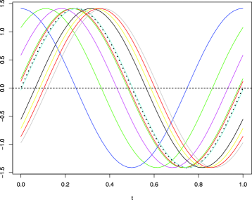
Figure 1: Ten simulated EFPC’s $\hat{v}_{1}$ for process (22) with $\lambda=0.5$ and $e_{1}(t)=\sqrt{2}\sin(2\uppi t)$, $e_{2}(t)=\sqrt{2}\cos(2\uppi t)$ ($N=100$). The dotted line is the population eigenfunction.

Ten simulated $\hat{v}_{1}$ are shown in Figure 1. To compute each $\hat{v}_{1}$, we simulated curves $X(s_{n})$ given by (22) with with $e_{1}(t)=\sqrt{2}\sin(2\uppi t),e_{2}(t)=\sqrt{2}\cos(2\uppi t)$, $\lambda=0.5$. We set $s_{n}=n^{-1},n=1,2,\ldots,N,N=100$. The random vectors $[\zeta_{j}(s_{1}),\zeta_{j}(s_{2}),\ldots,\zeta_{j}(s_{N})]^{T}$ were generated using the R function rmvnorm which uses the singular value decomposition to simulate Gaussian vectors with predetermined covariances (in our case, $\operatorname{Cov}(\zeta_{j}(s_{k}),\zeta_{j}(s_{\ell}))=\exp\{-|k^{-1}-\ell^{-1}|\}$).

The EFPC $\hat{v}_{1}$ is a linear combination of $e_{1}$ and $e_{2}$ with random weights. As formula (23) suggests, the function $e_{1}$ is likely to receive a larger weight. The weights, and so the simulated $\hat{v}_{1}$, cluster because both $Z_{1}$ and $Z_{2}$ are standard normal.

We now state a general result showing that Type A sampling generally leads to inconsistent estimators if the spatial dependence does not vanish.

Proposition 9

Assume that $E\langle X(\mathbf{s}_{1})-\mu,X(\mathbf{s}_{2})-\mu\rangle\geq b(\|\mathbf{s}_{1}-\mathbf{s}_{2}\|_{2})>0$, where $b(x)$ is non-increasing. Then under Type A sampling the sample mean $\bar{X}_{N}$ is not a consistent estimator of $\mu$. Similarly, if $EX(\mathbf{s})=0$ and

$$E\langle X(\mathbf{s}_{1})\otimes X(\mathbf{s}_{1})-C,X(\mathbf{s}_{2})\otimes X(\mathbf{s}_{2})-C\rangle_{\mathcal{S}}\geq B(\|\mathbf{s}_{1}-\mathbf{s}_{2}\|_{2})>0,$$ (24)

where $B(x)$ is nonincreasing, then under Type A sampling the sample covariance $\widehat{C}_{N}$ is not a consistent estimator of $C$.

We illustrate Proposition 9 with a further example that complements Proposition 8 in a sense that in Proposition 8 the functional model was complex, but the spatial distribution of the $\mathbf{s}_{k}$ simple. In Example 8, we allow a general Type A distribution, but consider the simple model (22).

Example 8.

We focus on condition (24) for the FPC’s. For the general model (8), the left-hand side of (24) is equal to

$$\kappa(\mathbf{s}_{1},\mathbf{s}_{2})=\sum_{i,j\geq 1}\operatorname{Cov}(\xi_{i}(\mathbf{s}_{1})\xi_{j}(\mathbf{s}_{1}),\xi_{i}(\mathbf{s}_{2})\xi_{j}(\mathbf{s}_{2})).$$

If the processes $\xi_{j}$ satisfy the assumptions of Proposition 8, then, by Lemma 4,

$$\operatorname{Cov}(\xi_{i}(\mathbf{s}_{1})\xi_{j}(\mathbf{s}_{1}),\xi_{i}(\mathbf{s}_{2})\xi_{j}(\mathbf{s}_{2}))=\lambda_{i}^{2}r_{i}+\lambda_{j}^{2}r_{j}+\lambda_{i}\lambda_{j}\frac{r_{i}+r_{j}}{2}-(\lambda_{i}^{3/2}r_{i}+\lambda_{j}^{3/2}r_{j})\sqrt{\lambda_{i}+\lambda_{j}},$$

where $r_{i}=\rho_{i}(\|\mathbf{s}_{1}-\mathbf{s}_{2}\|)$.

To calculate $\kappa(\mathbf{s}_{1},\mathbf{s}_{2})$ in a simple case, corresponding to (22), suppose

$$\lambda_{1}=1,\qquad\lambda_{2}=\lambda,\qquad 0<\lambda<1,\qquad\lambda_{i}=0,\qquad i>2\quad\mbox{and}\quad\rho_{1}=\rho_{2}=\rho.$$ (25)

Then,

$$\kappa(\mathbf{s}_{1},\mathbf{s}_{2})=f(\lambda)\rho(\|\mathbf{s}_{1}-\mathbf{s}_{2}\|),$$

where

$$f(\lambda)=\bigl{(}3-2\sqrt{2}\bigr{)}(1+\lambda^{2})+2[1+\lambda+\lambda^{2}-(1+\lambda^{3/2})(1+\lambda)^{1/2}].$$

The function $f$ increases from about 0.17 at $\lambda=0$ to about 0.69 at $\lambda=1$.

We have verified that if the functional random field (8) satisfies the assumptions of Proposition 8 and (25), then $\widehat{C}_{N}$ is an inconsistent estimator of $C$ under Type A sampling, whenever $\rho(h)$ is a nonincreasing function of $h$.

6 Proofs of the results of Sections 3, 4 and 5

We will use the following well-known lemma.

Lemma 4

Suppose $X$ and $Y$ are jointly normal mean zero random variables such that $EX^{2}=\sigma^{2},EY^{2}=\nu^{2},E[XY]=\rho\sigma\nu.$ Then

$$\operatorname{Cov}(X^{2},Y^{2})=2\rho^{2}\sigma^{2}\nu^{2}.$$

Proof of Proposition 1 By Assumption 1, we have

$$E\Biggl{\|}\frac{1}{N}\sum_{k=1}^{N}X(\mathbf{s}_{k,N})-\mu\Biggr{\|}^{2}$$

$$\quad=\frac{1}{N^{2}}\sum_{k=1}^{N}\sum_{\ell=1}^{N}E\langle X(\mathbf{s}_{k,N})-\mu,X(\mathbf{s}_{\ell,N})-\mu\rangle$$

$$\quad\leq\frac{1}{N^{2}}\sum_{k=1}^{N}\sum_{\ell=1}^{N}h(\|\mathbf{s}_{k,N}-\mathbf{s}_{\ell,N}\|_{2})$$

$$\quad\leq\frac{1}{N^{2}}\sum_{k=1}^{N}\sum_{\ell=1}^{N}\bigl{(}h(\rho_{N})I\{\|\mathbf{s}_{k,N}-\mathbf{s}_{\ell,N}\|_{2}\geq\rho_{N}\}+h(0)I\{\|\mathbf{s}_{k,N}-\mathbf{s}_{\ell,N}\|_{2}\leq\rho_{N}\}\bigr{)}$$

$$\quad\leq h(\rho_{N})+h(0)I_{\rho_{N}}(\mathfrak{S}_{N}).$$

The following lemma is a simple calculus problem and will be used in the proof of Proposition 2.

Lemma 5

Assume that $f$ is a nonnegative function which is monotone on $[0,b]$ and on $[b,\infty)$. Then

$$\sum_{k=0}^{L}f\biggl{(}\frac{k}{N}\biggr{)}\frac{1}{N}\leq\int_{0}^{L/N}f(x)\,\mathrm{d}x+\frac{2}{N}\sup_{x\in[0,L/N]}|f(x)|.$$

Proof of Proposition 2 By Assumption 1,

$$E\Biggl{\|}\frac{1}{S_{N}}\sum_{k=1}^{S_{N}}X(\mathbf{s}_{k,N})-\mu\Biggr{\|}^{2}\leq\frac{1}{S_{N}^{2}}\sum_{k=1}^{S_{N}}\sum_{\ell=1}^{S_{N}}h(\|\mathbf{s}_{k,N}-\mathbf{s}_{\ell,N}\|_{2}).$$

Let $\mathbf{a}=(a_{1},\ldots,a_{d})$ and $\mathbf{b}=(b_{1},\ldots,b_{d})$ be two elements on $\mathcal{Z}(\bm{\delta})$. We define $d(\mathbf{a},\mathbf{b})=\min_{1\leq i\leq d}v_{i}(\mathbf{a},\mathbf{b})$, where $v_{i}(\mathbf{a},\mathbf{b})$ is the number of edges between $a_{i}$ and $b_{i}$. For any two points $\mathbf{s}_{k,N}$ and $\mathbf{s}_{\ell,N}$, we have

$$d(\mathbf{s}_{k,N},\mathbf{s}_{\ell,N})=m\qquad\mbox{from some }m\in\{0,\ldots,KN^{1/d}\},$$ (26)

where $K$ depends on $\operatorname{diam}(R_{0})$. It is easy to see that the number of points on the grid having distance $m$ from a given point is less than $2d(2m+1)^{d}$, $m\geq 0$. Hence, the number of pairs for which (26) holds is $<2d(2m+1)^{d-1}N$. On the other hand, if $d(\mathbf{s}_{k,N},\mathbf{s}_{\ell,N})=m$, then $\|\mathbf{s}_{k,N}-\mathbf{s}_{\ell,N}\|_{2}\geq m\delta_{0}\eta_{N}$. Let us assume without loss of generality that $\delta_{0}=1$. Noting that there is no loss of generality if we assume that $x^{\delta-1}h(x)$ is also monotone on $[0,b]$, we obtain by Lemma 5 for large enough $N$ and $K<K^{\prime}<K^{\prime\prime}$

$$\frac{1}{S_{N}^{2}}\sum_{k=1}^{S_{N}}\sum_{\ell=1}^{S_{N}}h(\|\mathbf{s}_{k,N}-\mathbf{s}_{\ell,n}\|_{2})$$

$$\quad\leq 2d\sum_{m=1}^{K^{\prime}N^{1/d}}\frac{(2m+1)^{d-1}}{N}h(m\eta_{N})+\frac{2h(0)}{N}$$

$$\quad\leq 2d\biggl{(}\frac{3}{\eta_{N}}\biggr{)}^{d-1}\sum_{m=0}^{K^{\prime}N^{1/d}+1}\biggl{(}\frac{m}{N}N\eta_{N}\biggr{)}^{d-1}h\biggl{(}\frac{m}{N}N\eta_{N}\biggr{)}\frac{1}{N}+\frac{2h(0)}{N}$$

$$\quad\leq 2d\biggl{(}\frac{3}{\eta_{N}}\biggr{)}^{d-1}\biggl{(}\int_{0}^{K^{\prime\prime}N^{1/d-1}}(N\eta_{N}x)^{d-1}h(N\eta_{N}x)\,\mathrm{d}x$$

$$\hphantom{\quad\leq 2d\biggl{(}\frac{3}{\eta_{N}}\biggr{)}^{d-1}\biggl{(}}{}+\frac{2}{N}\sup_{x\in[0,K^{\prime\prime}\alpha_{N}/\Delta]}x^{d-1}h(x)\biggr{)}+\frac{2h(0)}{N}$$

$$\quad=\frac{(3\Delta)^{d}d}{\alpha_{N}^{d}}\int_{0}^{K^{\prime\prime}\alpha_{N}/\Delta}x^{d-1}h(x)\,\mathrm{d}x$$

$$\qquad{}+\frac{4d(3\Delta)^{d-1}}{\alpha_{N}^{d-1}N^{1/d}}\sup_{x\in[0,K^{\prime\prime}\alpha_{N}/\Delta]}x^{d-1}h(x)+\frac{2h(0)}{N}.$$

By Lemma 2, Type B sampling implies $\alpha_{N}\to\infty$ and $\alpha_{N}=\mathrm{o}(N^{1/d})$. This shows (2). Under Type C sampling $1/\alpha_{N}^{d}\ll 1/N$. The proof is finished. Proof of Proposition 3 This time we have

$$E\Biggl{\|}\frac{1}{N}\sum_{k=1}^{N}X(\mathbf{s}_{k,N})-\mu\Biggr{\|}^{2} \leq \frac{1}{N^{2}}\sum_{k=1}^{N}\sum_{\ell=1}^{N}Eh(\|\mathbf{s}_{k,N}-\mathbf{s}_{\ell,N}\|_{2})$$

$$\leq \alpha_{N}^{-2d}\int_{R_{N}}\int_{R_{N}}h(\|\mathbf{s}-\mathbf{r}\|_{2})f(\alpha_{N}^{-1}\mathbf{s})f(\alpha_{N}^{-1}\mathbf{r})\,\mathrm{d}\mathbf{s}\,\mathrm{d}\mathbf{r}+\frac{h(0)}{N}$$

$$= \int_{R_{0}}\int_{R_{0}}h(\alpha_{N}\|\mathbf{s}-\mathbf{r}\|_{2})f(\mathbf{s})f(\mathbf{r})\,\mathrm{d}\mathbf{s}\,\mathrm{d}\mathbf{r}+\frac{h(0)}{N}.$$

Furthermore, for any $\varepsilon_{N}>0$,

$$\int_{R_{0}}\int_{R_{0}}h(\alpha_{N}\|\mathbf{s}-\mathbf{r}\|_{2})f(\mathbf{s})f(\mathbf{r})\,\mathrm{d}\mathbf{s}\,\mathrm{d}\mathbf{r}$$

$$\quad\leq h(0)\int_{R_{0}}\int_{R_{0}}f(\mathbf{s})f(\mathbf{r})I\{\|\mathbf{s}-\mathbf{r}\|_{2}\leq\varepsilon_{N}\}\,\mathrm{d}\mathbf{s}\,\mathrm{d}\mathbf{r}+h(\alpha_{N}\varepsilon_{N})$$

$$\quad\leq h(0)\sup_{\mathbf{s}\in R_{0}}f^{2}(\mathbf{s})\times\int_{R_{0}}\int_{R_{0}}I\{\|\mathbf{s}-\mathbf{r}\|_{2}\leq\varepsilon_{N}\}\,\mathrm{d}\mathbf{s}\,\mathrm{d}\mathbf{r}+h(\alpha_{N}\varepsilon_{N}).$$

Now for fixed $\mathbf{r}$ it is not difficult to show that $\int_{R_{0}}I\{\|\mathbf{s}-\mathbf{r}\|_{2}\leq\varepsilon_{N}\}\,\mathrm{d}\mathbf{s}\leq 6\varepsilon_{N}^{d}$. (The constant 6 could be replaced with $\uppi^{d/2}/\Gamma(d/2+1))$. Proof of Proposition 8 Observe that

$$\|\widehat{C}_{N}-X^{\star}\|_{\mathcal{S}}^{2}=\int\!\!\!\int\Biggl{\{}\frac{1}{N}\sum_{n=1}^{N}[X(\mathbf{s}_{n};t)X(\mathbf{s}_{n};u)-X(\bm{0};t)X(\bm{0};u)]\Biggr{\}}^{2}\,\mathrm{d}t\,\mathrm{d}u.$$

Therefore,

$$\|\widehat{C}_{N}-X^{\star}\|_{\mathcal{S}}^{2}\leq 2I_{1}(N)+2I_{2}(N),$$

where

$$I_{1}(N)=\int\!\!\!\int\Biggl{\{}\frac{1}{N}\sum_{n=1}^{N}X(\mathbf{s}_{n};t)\bigl{(}X(\mathbf{s}_{n};u)-X(\bm{0};u)\bigr{)}\Biggr{\}}^{2}\,\mathrm{d}t\,\mathrm{d}u$$

and

$$I_{2}(N)=\int\!\!\!\int\Biggl{\{}\frac{1}{N}\sum_{n=1}^{N}X(\bm{0};u)\bigl{(}X(\mathbf{s}_{n};t)-X(\bm{0};t)\bigr{)}\Biggr{\}}^{2}\,\mathrm{d}t\,\mathrm{d}u.$$

We will show that $EI_{1}(N)\to 0$. The argument for $I_{2}(N)$ is the same. Observe that

$$I_{1}(N) = \frac{1}{N^{2}}\sum_{k,\ell=1}^{N}\int\!\!\!\int X(\mathbf{s}_{k};t)\bigl{(}X(\mathbf{s}_{k};u)-X(\bm{0};u)\bigr{)}X(\mathbf{s}_{\ell};t)\bigl{(}X(\mathbf{s}_{\ell};u)-X(\bm{0};u)\bigr{)}\,\mathrm{d}t\,\mathrm{d}u$$

$$= \frac{1}{N^{2}}\sum_{k,\ell=1}^{N}\int X(\mathbf{s}_{k};t)X(\mathbf{s}_{\ell};t)\,\mathrm{d}t\int\bigl{(}X(\mathbf{s}_{k};u)-X(\bm{0};u)\bigr{)}\bigl{(}X(\mathbf{s}_{\ell};u)-X(\bm{0};u)\bigr{)}\,\mathrm{d}u.$$

Thus,

$$EI_{1}(N)\leq\frac{1}{N^{2}}\sum_{k,\ell=1}^{N}\biggl{\{}E\biggl{(}\int X(\mathbf{s}_{k};t)X(\mathbf{s}_{\ell};t)\,\mathrm{d}t\biggr{)}^{2}\biggr{\}}^{1/2}\biggl{\{}E\biggl{(}\int Y_{k}(u)Y_{\ell}(u)\,\mathrm{d}u\biggr{)}^{2}\biggr{\}}^{1/2},$$

where

$$Y_{k}(u)=X(\mathbf{s}_{k};u)-X(\bm{0};u).$$

We first deal with the integration over $t$:

$$E\biggl{(}\int X(\mathbf{s}_{k};t)X(\mathbf{s}_{\ell};t)\,\mathrm{d}t\biggr{)}^{2} \leq E\int X^{2}(\mathbf{s}_{k};t)\,\mathrm{d}t\int X^{2}(\mathbf{s}_{\ell};t)\,\mathrm{d}t=E[\|X(\mathbf{s}_{k})\|^{2}\|X(\mathbf{s}_{\ell})\|^{2}]$$

$$\leq \{E\|X(\mathbf{s}_{k})\|^{4}\}^{1/2}\{E\|X(\mathbf{s}_{\ell})\|^{4}\}^{1/2}=E\|X(\bm{0})\|^{4}.$$

We thus see that

$$EI_{1}(N) \leq \{E\|X(\bm{0})\|^{4}\}^{1/2}\frac{1}{N^{2}}\sum_{k,\ell=1}^{N}\biggl{\{}E\biggl{(}\int Y_{k}(u)Y_{\ell}(u)\,\mathrm{d}u\biggr{)}^{2}\biggr{\}}^{1/2}$$

$$\leq \{E\|X(\bm{0})\|^{4}\}^{1/2}\frac{1}{N^{2}}\sum_{k,\ell=1}^{N}\biggl{\{}E\biggl{(}\int Y_{k}^{2}(u)\,\mathrm{d}u\biggr{)}^{2}\biggr{\}}^{1/4}\biggl{\{}E\biggl{(}\int Y_{\ell}^{2}(u)\,\mathrm{d}u\biggr{)}^{2}\biggr{\}}^{1/4}$$

$$= \{E\|X(\bm{0})\|^{4}\}^{1/2}\Biggl{[}\frac{1}{N}\sum_{k=1}^{N}\biggl{\{}E\biggl{(}\int Y_{k}^{2}(u)\,\mathrm{d}u\biggr{)}^{2}\biggr{\}}^{1/4}\Biggr{]}^{2}.$$

Consequently, to complete the verification of (21), it suffices to show that

$$\lim_{N\to\infty}\frac{1}{N}\sum_{k=1}^{N}\biggl{\{}E\biggl{(}\int Y_{k}^{2}(u)\,\mathrm{d}u\biggr{)}^{2}\biggr{\}}^{1/4}=0.$$

The above relation will follow from

$$\lim_{k\to\infty}E\biggl{(}\int Y_{k}^{2}(u)\,\mathrm{d}u\biggr{)}^{2}=0.$$ (27)

To verify (27), first notice that, by the orthonormality of the $e_{j}$,

$$\int Y_{k}^{2}(u)\,\mathrm{d}u=\sum_{j=1}^{\infty}\bigl{(}\xi_{j}(\mathbf{s}_{k})-\xi_{j}(\bm{0})\bigr{)}^{2}.$$

Therefore, by the independence of the processes $\xi_{j}$,

$$E\biggl{(}\int Y_{k}^{2}(u)\,\mathrm{d}u\biggr{)}^{2} = \sum_{j=1}^{\infty}E\bigl{(}\xi_{j}(\mathbf{s}_{k})-\xi_{j}(\bm{0})\bigr{)}^{4}$$

$${}+\sum_{i\neq j}E\bigl{(}\xi_{i}(\mathbf{s}_{k})-\xi_{i}(\bm{0})\bigr{)}^{2}E\bigl{(}\xi_{j}(\mathbf{s}_{k})-\xi_{j}(\bm{0})\bigr{)}^{2}.$$

The covariance structure was specified so that

$$E\bigl{(}\xi_{j}(\mathbf{s}_{k})-\xi_{j}(\bm{0})\bigr{)}^{2}=2\lambda_{j}\bigl{(}1-\rho_{j}(\|\mathbf{s}_{k}\|)\bigr{)},$$

so the normality yields

$$E\biggl{(}\int Y_{k}^{2}(u)\,\mathrm{d}u\biggr{)}^{2} \leq 12\sum_{j=1}^{\infty}\lambda_{j}^{2}\bigl{(}1-\rho_{j}(\|\mathbf{s}_{k}\|)\bigr{)}^{2}$$

$${}+4\Biggl{\{}\sum_{j=1}^{\infty}\lambda_{j}\bigl{(}1-\rho_{j}(\|\mathbf{s}_{k}\|)\bigr{)}\Biggr{\}}^{2}.$$

The right-hand side tends to zero by the Dominated Convergence theorem. This establishes (27), and completes the proof of (21). Proof of Proposition 9 We only check inconsistency of the sample mean. In view of the proof of Proposition 1, we have now the lower bound

$$E\Biggl{\|}\frac{1}{N}\sum_{k=1}^{N}X(\mathbf{s}_{k,N})-\mu\Biggr{\|}^{2} \geq \frac{1}{N^{2}}\sum_{k=1}^{N}\sum_{\ell=1}^{N}b(\|\mathbf{s}_{k,N}-\mathbf{s}_{\ell,N}\|_{2})$$

$$\geq b(\rho)I_{\rho}^{2}(\mathfrak{S}_{N}),$$

which is by assumption bounded away from zero for $N\to\infty$.

References

- [1] {barticle}[mr] \bauthor\bsnmBel, \bfnmLiliane\binitsL., \bauthor\bsnmBar-Hen, \bfnmAvner\binitsA., \bauthor\bsnmPetit, \bfnmRémy\binitsR. &\bauthor\bsnmCheddadi, \bfnmRachid\binitsR. (\byear2011). \btitleSpatio-temporal functional regression on paleoecological data. \bjournalJ. Appl. Stat. \bvolume38 \bpages695–704. \biddoi=10.1080/02664760903563650, issn=0266-4763, mr=2773575 \bptokimsref \endbibitem
- [2] {barticle}[mr] \bauthor\bsnmBenko, \bfnmMichal\binitsM., \bauthor\bsnmHärdle, \bfnmWolfgang\binitsW. &\bauthor\bsnmKneip, \bfnmAlois\binitsA. (\byear2009). \btitleCommon functional principal components. \bjournalAnn. Statist. \bvolume37 \bpages1–34. \biddoi=10.1214/07-AOS516, issn=0090-5364, mr=2488343 \bptokimsref \endbibitem
- [3] {barticle}[mr] \bauthor\bsnmBolthausen, \bfnmE.\binitsE. (\byear1982). \btitleOn the central limit theorem for stationary mixing random fields. \bjournalAnn. Probab. \bvolume10 \bpages1047–1050. \bidissn=0091-1798, mr=0672305 \bptokimsref \endbibitem
- [4] {bbook}[mr] \bauthor\bsnmBosq, \bfnmD.\binitsD. (\byear2000). \btitleLinear Processes in Function Spaces: Theory and Applications. \bseriesLecture Notes in Statistics \bvolume149. \baddressNew York: \bpublisherSpringer. \bidmr=1783138 \bptokimsref \endbibitem
- [5] {bbook}[mr] \bauthor\bsnmCressie, \bfnmNoel A. C.\binitsN.A.C. (\byear1993). \btitleStatistics for Spatial Data. \bseriesWiley Series in Probability and Mathematical Statistics: Applied Probability and Statistics. \baddressNew York: \bpublisherWiley. \bnoteRevised reprint of the 1991 edition, A Wiley-Interscience Publication. \bidmr=1239641 \bptokimsref \endbibitem
- [6] {barticle}[mr] \bauthor\bsnmDelicado, \bfnmP.\binitsP., \bauthor\bsnmGiraldo, \bfnmR.\binitsR., \bauthor\bsnmComas, \bfnmC.\binitsC. &\bauthor\bsnmMateu, \bfnmJ.\binitsJ. (\byear2010). \btitleStatistics for spatial functional data: Some recent contributions. \bjournalEnvironmetrics \bvolume21 \bpages224–239. \biddoi=10.1002/env.1003, issn=1180-4009, mr=2842240 \bptokimsref \endbibitem
- [7] {barticle}[mr] \bauthor\bsnmDu, \bfnmJuan\binitsJ., \bauthor\bsnmZhang, \bfnmHao\binitsH. &\bauthor\bsnmMandrekar, \bfnmV. S.\binitsV.S. (\byear2009). \btitleFixed-domain asymptotic properties of tapered maximum likelihood estimators. \bjournalAnn. Statist. \bvolume37 \bpages3330–3361. \biddoi=10.1214/08-AOS676, issn=0090-5364, mr=2549562 \bptokimsref \endbibitem
- [8] {barticle}[mr] \bauthor\bsnmEinmahl, \bfnmJ. H. J.\binitsJ.H.J. &\bauthor\bsnmRuymgaart, \bfnmF. H.\binitsF.H. (\byear1987). \btitleThe order of magnitude of the moments of the modulus of continuity of multiparameter Poisson and empirical processes. \bjournalJ. Multivariate Anal. \bvolume21 \bpages263–273. \biddoi=10.1016/0047-259X(87)90005-4, issn=0047-259X, mr=0884100 \bptokimsref \endbibitem
- [9] {barticle}[mr] \bauthor\bsnmGabrys, \bfnmRobertas\binitsR., \bauthor\bsnmHorváth, \bfnmLajos\binitsL. &\bauthor\bsnmKokoszka, \bfnmPiotr\binitsP. (\byear2010). \btitleTests for error correlation in the functional linear model. \bjournalJ. Amer. Statist. Assoc. \bvolume105 \bpages1113–1125. \biddoi=10.1198/jasa.2010.tm09794, issn=0162-1459, mr=2752607 \bptokimsref \endbibitem
- [10] {barticle}[mr] \bauthor\bsnmGabrys, \bfnmRobertas\binitsR. &\bauthor\bsnmKokoszka, \bfnmPiotr\binitsP. (\byear2007). \btitlePortmanteau test of independence for functional observations. \bjournalJ. Amer. Statist. Assoc. \bvolume102 \bpages1338–1348. \biddoi=10.1198/016214507000001111, issn=0162-1459, mr=2412554 \bptokimsref \endbibitem
- [11] {bmisc}[auto:STB—2012/03/21—07:41:58] \bauthor\bsnmGohberg, \bfnmI.\binitsI., \bauthor\bsnmGolberg, \bfnmS.\binitsS. &\bauthor\bsnmKaashoek, \bfnmM. A.\binitsM.A. (\byear1990). \bhowpublishedClasses of Linear Operators. Operator Theory: Advances and Applications 49. Basel: Birkhaüser. \bptokimsref \endbibitem
- [12] {barticle}[mr] \bauthor\bsnmHall, \bfnmPeter\binitsP. &\bauthor\bsnmHosseini-Nasab, \bfnmMohammad\binitsM. (\byear2006). \btitleOn properties of functional principal components analysis. \bjournalJ. R. Stat. Soc. Ser. B Stat. Methodol. \bvolume68 \bpages109–126. \biddoi=10.1111/j.1467-9868.2005.00535.x, issn=1369-7412, mr=2212577 \bptokimsref \endbibitem
- [13] {barticle}[mr] \bauthor\bsnmHörmann, \bfnmSiegfried\binitsS. &\bauthor\bsnmKokoszka, \bfnmPiotr\binitsP. (\byear2010). \btitleWeakly dependent functional data. \bjournalAnn. Statist. \bvolume38 \bpages1845–1884. \biddoi=10.1214/09-AOS768, issn=0090-5364, mr=2662361 \bptokimsref \endbibitem
- [14] {bmisc}[auto:STB—2012/03/21—07:41:58] \bauthor\bsnmHörmann, \bfnmS.\binitsS. &\bauthor\bsnmKokoszka, \bfnmP.\binitsP. (\byear2012). \bhowpublishedSupplement to “Consistency of the mean and the principal components of spatially distributed functional data.” DOI:\doiurl10.3150/12-BEJ418SUPP. \bptokimsref \endbibitem
- [15] {barticle}[mr] \bauthor\bsnmJenish, \bfnmNazgul\binitsN. &\bauthor\bsnmPrucha, \bfnmIngmar R.\binitsI.R. (\byear2009). \btitleCentral limit theorems and uniform laws of large numbers for arrays of random fields. \bjournalJ. Econometrics \bvolume150 \bpages86–98. \biddoi=10.1016/j.jeconom.2009.02.009, issn=0304-4076, mr=2525996 \bptokimsref \endbibitem
- [16] {barticle}[mr] \bauthor\bsnmJiang, \bfnmCi-Ren\binitsC.R. &\bauthor\bsnmWang, \bfnmJane-Ling\binitsJ.L. (\byear2010). \btitleCovariate adjusted functional principal components analysis for longitudinal data. \bjournalAnn. Statist. \bvolume38 \bpages1194–1226. \biddoi=10.1214/09-AOS742, issn=0090-5364, mr=2604710 \bptokimsref \endbibitem
- [17] {barticle}[mr] \bauthor\bsnmLahiri, \bfnmSoumendra Nath\binitsS.N. (\byear1996). \btitleOn inconsistency of estimators based on spatial data under infill asymptotics. \bjournalSankhyā Ser. A \bvolume58 \bpages403–417. \bidissn=0581-572X, mr=1659130 \bptokimsref \endbibitem
- [18] {barticle}[mr] \bauthor\bsnmLahiri, \bfnmS. N.\binitsS.N. (\byear2003). \btitleCentral limit theorems for weighted sums of a spatial process under a class of stochastic and fixed designs. \bjournalSankhyā \bvolume65 \bpages356–388. \bidissn=0972-7671, mr=2028905 \bptokimsref \endbibitem
- [19] {barticle}[mr] \bauthor\bsnmLahiri, \bfnmS. N.\binitsS.N. &\bauthor\bsnmZhu, \bfnmJun\binitsJ. (\byear2006). \btitleResampling methods for spatial regression models under a class of stochastic designs. \bjournalAnn. Statist. \bvolume34 \bpages1774–1813. \biddoi=10.1214/009053606000000551, issn=0090-5364, mr=2283717 \bptokimsref \endbibitem
- [20] {barticle}[mr] \bauthor\bsnmLoh, \bfnmWei-Liem\binitsW.L. (\byear2005). \btitleFixed-domain asymptotics for a subclass of Matérn-type Gaussian random fields. \bjournalAnn. Statist. \bvolume33 \bpages2344–2394. \biddoi=10.1214/009053605000000516, issn=0090-5364, mr=2211089 \bptokimsref \endbibitem
- [21] {barticle}[mr] \bauthor\bsnmPark, \bfnmByeong U.\binitsB.U., \bauthor\bsnmKim, \bfnmTae Yoon\binitsT.Y., \bauthor\bsnmPark, \bfnmJeong-Soo\binitsJ.S. &\bauthor\bsnmHwang, \bfnmS. Y.\binitsS.Y. (\byear2009). \btitlePractically applicable central limit theorem for spatial statistics. \bjournalMath. Geosci. \bvolume41 \bpages555–569. \biddoi=10.1007/s11004-008-9184-2, issn=1874-8961, mr=2516125 \bptokimsref \endbibitem
- [22] {barticle}[mr] \bauthor\bsnmPaul, \bfnmDebashis\binitsD. &\bauthor\bsnmPeng, \bfnmJie\binitsJ. (\byear2009). \btitleConsistency of restricted maximum likelihood estimators of principal components. \bjournalAnn. Statist. \bvolume37 \bpages1229–1271. \biddoi=10.1214/08-AOS608, issn=0090-5364, mr=2509073 \bptokimsref \endbibitem
- [23] {bmisc}[auto:STB—2012/03/21—07:41:58] \bauthor\bsnmRamsay, \bfnmJ.\binitsJ., \bauthor\bsnmHooker, \bfnmG.\binitsG. &\bauthor\bsnmGraves, \bfnmS.\binitsS. (\byear2009). \bhowpublishedFunctional Data Analysis with R and MATLAB. New York: Springer. \bptokimsref \endbibitem
- [24] {bbook}[mr] \bauthor\bsnmRamsay, \bfnmJ. O.\binitsJ.O. &\bauthor\bsnmSilverman, \bfnmB. W.\binitsB.W. (\byear2005). \btitleFunctional Data Analysis, \bedition2nd ed. \bseriesSpringer Series in Statistics. \baddressNew York: \bpublisherSpringer. \bidmr=2168993 \bptokimsref \endbibitem
- [25] {barticle}[mr] \bauthor\bsnmReiss, \bfnmPhilip T.\binitsP.T. &\bauthor\bsnmOgden, \bfnmR. Todd\binitsR.T. (\byear2007). \btitleFunctional principal component regression and functional partial least squares. \bjournalJ. Amer. Statist. Assoc. \bvolume102 \bpages984–996. \biddoi=10.1198/016214507000000527, issn=0162-1459, mr=2411660 \bptokimsref \endbibitem
- [26] {barticle}[mr] \bauthor\bsnmRio, \bfnmEmmanuel\binitsE. (\byear1993). \btitleCovariance inequalities for strongly mixing processes. \bjournalAnn. Inst. Henri Poincaré Probab. Stat. \bvolume29 \bpages587–597. \bidissn=0246-0203, mr=1251142 \bptokimsref \endbibitem
- [27] {bbook}[mr] \bauthor\bsnmStein, \bfnmMichael L.\binitsM.L. (\byear1999). \btitleInterpolation of Spatial Data: Some Theory for Kriging. \bseriesSpringer Series in Statistics. \baddressNew York: \bpublisherSpringer. \bidmr=1697409 \bptokimsref \endbibitem
- [28] {barticle}[mr] \bauthor\bsnmStute, \bfnmWinfried\binitsW. (\byear1984). \btitleThe oscillation behavior of empirical processes: The multivariate case. \bjournalAnn. Probab. \bvolume12 \bpages361–379. \bidissn=0091-1798, mr=0735843 \bptokimsref \endbibitem
- [29] {barticle}[mr] \bauthor\bsnmYamanishi, \bfnmYoshihiro\binitsY. &\bauthor\bsnmTanaka, \bfnmYutaka\binitsY. (\byear2003). \btitleGeographically weighted functional multiple regression analysis: A numerical investigation. \bjournalJ. Japanese Soc. Comput. Statist. \bvolume15 \bpages307–317. \bidissn=0915-2350, mr=2027947 \bptokimsref \endbibitem
- [30] {barticle}[mr] \bauthor\bsnmZhang, \bfnmHao\binitsH. (\byear2004). \btitleInconsistent estimation and asymptotically equal interpolations in model-based geostatistics. \bjournalJ. Amer. Statist. Assoc. \bvolume99 \bpages250–261. \biddoi=10.1198/016214504000000241, issn=0162-1459, mr=2054303 \bptokimsref \endbibitem