Inplace Algorithm for Priority Search Tree and its use in Computing Largest Empty Axis-Parallel Rectangle

Abstract

There is a high demand of space-efficient algorithms in built-in or embedded softwares. In this paper, we consider the problem of designing space-efficient algorithms for computing the maximum area empty rectangle (MER) among a set of points inside a rectangular region $\cal R$ in 2D. We first propose an inplace algorithm for computing the priority search tree with a set of $n$ points in $\cal R$ using $O(\log n)$ extra bit space in $O(n\log n)$ time. It supports all the standard queries on priority search tree in $O(\log^{2}n)$ time. We also show an application of this algorithm in computing the largest empty axis-parallel rectangle. Our proposed algorithm needs $O(n\log^{2}n+m)$ time and $O(\log n)$ work-space apart from the array used for storing $n$ input points. Here $m$ is the number of maximal empty rectangles present in $\cal R$. Finally, we consider the problem of locating the maximum area empty rectangle of arbitrary orientation among a set of $n$ points, and propose an $O(n^{3}\log n)$ time in-place algorithm for that problem.

1 Introduction

Though memory is getting cheap day by day, still there are massive demand for the low memory algorithms for practical problems which need to be run on tiny devices, for example, sensors, GPS systems, mobile hand-sets, small robots, etc. Also, now-a-days the data available in several problems itself is huge. So, the practical algorithms for the data-streaming or data-mining problems must be space-efficient. For all these reasons, designing low-memory algorithms for practical problems have now become a challenging task in the algorithm research.

In computational geometry, designing the in-place algorithms are studied only for a very few problems. For convex hull problem in both 2D and 3D, space efficient algorithms are available. In 2D, the best known result is a $O(n\log h)$ algorithm with $O(1)$ extra space [5]. Bronnimann et al. [4] also showed that the upper hull of a set of $n$ points in 3D can be computed in $O(n\log^{3}n)$ time using $O(1)$ extra space. In the same paper it is also shown that for a parameter $s$ satisfying $c\log^{2}n\leq s\leq n$, ($c\geq 0$ is a constant), if $O(\frac{n}{s})$ space is allowed, then the convex hull for a set of $n$ points in 3D can be computed in in $O(ns)$ time. Vahrenhold [14] proposed an $O(n^{\frac{3}{2}}\log n)$ time and $O(1)$ extra space algorithm for the Klee’s measure problem, where the objective is to compute the union of $n$ axis-parallel rectangles of arbitrary sizes. Bose et al. [3] used in-place divide and conquer technique to solve the following three problems in 2D using $O(1)$ extra space: (i) a deterministic algorithm for the closest pair problem in $O(n\log n)$ time, (ii) a randomized algorithm for the bichromatic closest pair problem in $O(n\log n)$ expected time, and (iii) a deterministic $O(n\log n+k)$ time algorithm for the orthogonal line segment intersection computation problem. For arbitrary line segments intersection computation problem, two algorithms are available in [8]. If the input array can be used for storing intermediate results, then the problem can be solved in $O((n+k)\log n)$ time and $O(1)$ space. but, if the input array is not allowed to be destroyed, then the time complexity increases by a factor of $\log n$, and it also requires $O(\log^{2}n)$ extra space. Regarding the empty space recognition problem, it needs to be mentioned that all the Delauney triangles among a set of $n$ points can be computed in $O(n^{2})$ time using $O(1)$ space [2]. This, in turn, recognizes the largest empty circle among a point set with the same time complexity.

In this paper, we propose an in-place algorithm for constructing a priority search tree $\cal T$ [10] with the set of points $P$ in $\cal R$, $|P|=n$. This needs an additional $O(\log n)$ bits. We show that, the standard queries on priority search tree can be performed in it in $O(\log^{2}n)$ time. Priority search tree is a very important paradigm in geometric algorithms, as it has several important applications. Thus, our algorithm may aid in several problems in memory-restricted environment.

As an immediate application of our inplace priority search tree, we have considered the computation of largest empty axis-parallel rectangles among the points in $P$. Our proposed algorithm runs in $O(m+n\log^{2}n)$ time using $O(\log n)$ extra space. Here $m$ is the number of maximal empty axis-parallel rectangles (MERs) in $\cal R$. By maximal empty axis-parallel rectangle (MER), we mean an empty axis-parallel rectangle that is not containined in any other empty axis-parallel rectangle.

The problem of computing the largest MER was first introduced by Namaad et al. [11]. They showed that the number of MERs’ ($m$) among a set of $n$ points may be $O(n^{2})$ in the worst case; but if the points are randomly placed, then the expected value of $m$ is $O(n\log n)$. In the same paper, an algorithm for identifying the largest MER was proposed. The worst case time complexity of that algorithm is $O(min(n^{2},m\log n))$. Orlowski [13] proposed an easy to implement algorithm for finding the largest MER that runs in $O(m+n\log n)$ time. It inspects all the MERs’ present on the floor, and identifies the largest one. The best known algorithm for this problem runs in $O(n\log^{2}n)$ time in the worst case [1]. Same time complexity result holds for the recognition of the largest MER among a set of arbitrary polygonal obstacles [12]. Recently, Boland and Urrutia [6] gave an $O(n\log n)$ time algorithm for finding the largest MER inside an $n$-sided simple polygon. All these algorithms use $O(n)$ extra space.

Finally, we considered the problem of designing an in-place algorithm for computing the largest empty rectangle of arbitrary orientation among a set of $n$ points. It takes $O(n^{3}\log n)$ time with an $O(1)$ additional workspace. The best known algorithm for this problem in the literature runs in $O(n^{3})$ time and $O(n^{2})$ space [7].

2 In-place priority search tree

Let $P=\{p_{1},p_{2},\ldots,p_{n}\}$ be the given set of points in 2D, where $2^{k-1}\leq n<2^{k}$. The array that stores the points in $P$, is also referred to as $P$. The $i$-th array location will be referred as $P[i]$. We now define the priority search tree $\cal T$ recursively in a way that suits our in-place implementation.

The tree $\cal T$ has exactly $k$ levels. The level of root in $\cal T$ is considered to be the $k$-th level. The root represents the entire set of points $P$, and it stores the point $p^{*}$, where $y(p^{*})=\max_{p\in P}y(p)$. Its two children are the priority search tree with the set of points $P_{\ell}$ and $P_{r}$, where $P_{\ell}$ and $P_{r}$ are defined as follows: (i) let $m=2^{k-1}$. Compute $m$-th order statistics $x_{(m)}$ among the $x$-coordinates of the points of $P$. The set $P_{\ell}=\{p\in P\mid p\neq p^{*},x_{p}\leq x_{(m)}\}$, and $P_{r}=\{p\in P\mid p\neq p^{*},x_{p}>x_{(m)}\}$. Thus, $|P_{\ell}|=2^{k-1}-1$, $|P_{r}|=n-2^{k-1}$, and $P_{\ell}\cup P_{r}=P\setminus\{p^{*}\}$. In our modified definition of priority search tree, we assume that each node at level $i$ $(i\neq 0$) represents a tree of size $2^{i}-1$ except the rightmost node in that level. Observe that, at the level $k-1$, each of the two subtrees of $P_{\ell}$ are of size $2^{k-2}-1$. But for $P_{r}$, we may not always be able to construct two subtrees if $|P_{r}|\leq 2^{k-2}$. In that case, it has only the left subtree rooted at the point having maximum $y$-coordinate in the point set $P_{r}$; otherwise it has two subtrees.

In general, at any node of the $i$-th level, the root is as defined earlier. If $P^{\prime}$ denotes the set of points represented by that node, then the number of children of that node is (i) zero or (ii) one or (iii) two depending on whether (i) $|P^{\prime}|=1$, or (ii) $1<|P^{\prime}|\leq 2^{i-1}$ or (iii) $|P^{\prime}|>2^{i-1}$. In Case (i), it has no subtree. In Case (ii), it has only the left subtree, and its size is $|P^{\prime}|-1$. In Case (iii), it has both left and right subtrees, and their sizes are $2^{i-2}-1$ and $|P^{\prime}|-2^{i-2}$ respectively. We maintain an array $TAG$ with $2\log n$ cells, indexed by the levels of the tree $\cal T$. Each cell is of size 2 bits. The $TAG[i]$ is set to 0 or 1 or 2 depending on whether $\Theta_{i}$ = the number of nodes at level $i$ of $\cal T$ is equal to $2\Theta_{i-1}$ or $2\Theta_{i-1}-1$ or $2\Theta_{i-1}-2$. Note that, unlike the usual priority search tree [10], at each node the discriminating $x$-value among the points in two subtrees is not stored. Here, the method of deciding the search direction from a node will be decided by observing the inorder predecessor and successor of that node in $\cal T$.

2.1 In-place organization of $\cal T$

$\cal T$ is organized in a heap like structure. All its leaves appear in the same level; but unlike heap, a non-leaf node of $\cal T$ may have zero or one or two child(ren). In a particular level $i$, at most one node may have less than two children, and if such a node exists, it is the right-most node in that level. The root of $\cal T$ is stored in $P[1]$; it has always two children, stored in $P[2]$ and $P[3]$ respectively. In general, if all the nodes in $\cal T$ have two children except the leaves, then the children of $P[j]$ reside at $P[2j]$ and $P[2j+1]$. But, since at most one node in a level of $\cal T$ is permitted to have less than two children, we use $TAG$ bits to compute the address of the children of a node. If a node at level $i$, and stored at $P[j]$, has two children, they are available at $P[2j-\sum_{\alpha={i+1}}^{k}TAG[\alpha]]$ and $P[2j-\sum_{\alpha={i+1}}^{k}TAG[\alpha]+1]$ respectively. If $P[j]$ corresponds to the right-most node at level $i$, and $TAG[i]=1$, then its only child resides at $P[2j-\sum_{\alpha={i+1}}^{k}TAG[\alpha]]$.

2.2 Creation of $\cal T$

We first initialize $TAG[i]=0$ for all $i=1,2,\ldots,k$, where $k=\lfloor\log n\rfloor$. The computation of $\cal T$ is done in a breadth-first manner. In other words, all the nodes in a particular level $i$ are computed prior to computing the nodes of level $i+1$, for all $i=1,2,\ldots,k$. We compute $p^{*}=P[j]$ (say), where $y(P[j])=\max_{i=1}^{n}y(P[i])$ as the root of $\cal T$, and store it in $P[1]$ by swapping $P[1]$ and $P[j]$. Next we sort $P\setminus\{p^{*}\}$ in an in-place manner with $O(n)$ data movement [9]. Its first $2^{k-1}-1$ elements form the set $P_{\ell}$ for the left subtree ${\cal T}_{\ell}$, and the remaining $n-2^{k-1}-1$ points form the set $P_{r}$ for the right subtree ${\cal T}_{r}$. Next, we identify $p_{\ell}^{*}$ and $p_{r}^{*}$, the roots of ${\cal T}_{\ell}$ and ${\cal T}_{r}$ (as defined for $\cal T$). The point $p_{\ell}^{*}$ (resp. $p_{r}^{*}$) is swapped with $P[2]$ (resp. $P[3]$). Again we sort the points in $P\setminus\{p^{*},p_{\ell}^{*},p_{r}^{*}\}$ to compute the nodes in the next level. Note that, at this level, both the children of $p_{\ell}^{*}$ exists; but the number of children of $p_{r}^{*}$ may be zero or one or two. If the number of children of $p_{r}^{*}$ is one or zero, $TAG[2]$ is set to 1 or 2. The same process continues up to the $k$-th level. Since, at each level, a sorting is involved, we have the following result:

Lemma 1

For a given set $P$ of $n$ points, the tree $\cal T$ can be constructed in $O(n\log^{2}n)$ time.

2.3 Traversal of $\cal T$

The traversal in $\cal T$ starts from its root (at $P[1]$). At each step, it moves towards one of its children. If $\cal T$ is full, the children of a node (point) stored at $P[j]$ (at level $i$ of $\cal T$) are available at $P[2j]$ and $P[2j+1]$. But, since $\cal T$ may not be full, we need to use $TAG$ bits attached to each level of $\cal T$ for the traversal. We maintain an integer location $\Delta$ during the traversal of $\cal T$. While moving from level $i$ to level $i+1$, we add $TAG[i]$ with $\Delta$. It is already mentioned in the earlier subsection that, the left (resp. right) child of the node $P[j]$ are available at location $2j-\Delta$ (resp. $2j+1-\Delta$). Again, if $P[j]$ is the right-most node of a level of $\cal T$, it may have zero, one or two children, and this information is available at $TAG[i]$. If $P[j]$ is the right-most in its level $i$, and it has only one child, then the algorithm has to move towards its left child irrespective of the requirement (of moving towards left or right) in the algorithm.

3 Standard queries on priority search tree

We now show that the standard queries on the priority search tree [10] can be performed in $\cal T$ also in $O(\log^{2}n)$ time with $O(1)$ additional space.

3.1 MinXInRectangle($x_{0},x_{1},y_{1}$)

Three real numbers $x_{0}$, $x_{1}$ and $y_{1}$ are given. The objective is to find the point $p^{*}=(x^{*},y^{*})\in P$ with minimum $x$-coordinate among those points $p=(x,y)\in P$ satisfying $x_{0}\leq x\leq x_{1}$ and $y\geq y_{1}$.

Since the $x$-coordinate of the partitioning line at each node of $\cal T$ is not stored as in [10], the search direction from a node $p\in{\cal T}$ is decided by its inorder predecessor $p^{-}$ and inorder successor $p^{+}$.

While executing this query with the interval $[x_{0},x_{1}]$, we first find the discriminant node $\pi\in\cal T$ such that $x(\pi^{-})<x_{1}$ and $x(\pi^{+})>x_{0}$. If $y(\pi)<y_{1}$, then report that the search can not output a feasible point satisfying the query; otherwise the search proceeds to answer the query. We initialize two locations $p^{*}$ and $\Delta^{*}$ with $\pi$ and $\Delta$, where $p^{*}$ will contain the final answer, and $\Delta$ is the sum of $TAG$ bits computed during the traversal up to the node $\pi$. The search proceeds in both the subtrees of $\pi$. The traversal in the left subtree of $\pi$ starts with $p=\pi$. The actions taken at each node $p$ on the search path, and the choice of its child for the next move is decided as follows.

• If $y(p)<y_{1}$, the search stops. Otherwise, execute the following three steps.

• If $x_{0}\leq x(p)\leq x_{1}$ then assign $p^{*}=p$

• If the $x(p^{-})<x_{0}$, then set $p$ = right child of $p$.

• If the $x(p^{+})>x_{0}$, then set $p$ = left child of $p$

Using a similar procedure we traverse the right subtree of $\pi$ starting with $p=\pi$, and restoring the value of $\Delta$ at node $\pi$, which is stored in $\Delta^{*}$. Finally, $p^{*}$ is reported as the answer to the query.

Time complexity: Since here the search direction from a node $q$ is guided by $x(q^{-})$ and $x(q^{+})$, each move from a node to its descendant in the direction of the search takes $O(\log n)$ time. Note that, while, searching $q^{-}$ or $q^{+}$ of a node $q$, we copy $\Delta$ of $q$ at a scalar location $\Delta^{\prime}$, and perform the search as mentioned in subsection 2.3.

Since the total number of nodes to be traversed to report the answer or the non-existence of a feasible solution is $O(\log n)$, we have the following lemma:

Lemma 2

Using the in-place priority search tree on a set of $n$ points, the MinXInRectangle($x_{0},x_{1},y_{1}$) query can be answered in $O(\log^{2}n)$ time using $O(1)$ extra space.

3.2 MaxXInRectangle($x_{0},x_{1},y_{1}$)

Three real numbers $x_{0}$, $x_{1}$ and $y_{1}$ are given. The objective is to find the point $p^{*}=(x^{*},y^{*})\in P$ with maximum $x$-coordinate among those points $p=(x,y)\in P$ satisfying $x_{0}\leq x\leq x_{1}$ and $y\geq y_{1}$. This query can be answered in a similar manner as in MinXInRectangle query with same time and space complexity.

3.3 MaxYInXRange($x_{0},x_{1}$)

Given a pair of real numbers $x_{0}$ and $x_{1}$, find a point $p^{*}=(x^{*},y^{*})$ whose $y$ coordinate is maximum among all the points in $P$ satisfying $x_{0}\leq x\leq x_{1}$. Here the algorithm is essentially the same as in MinXInRectangle query. Here if a node satisfies $x_{0}\leq x\leq x_{1}$ during the search for the discriminant node, the search stops reporting that point. Otherwise, we need to search separately both the subtrees of the discriminant node till a point is obtained satisfying $x_{0}\leq x\leq x_{1}$. Surely, time and space complexities of MinXInRectangle query hold here also.

3.4 EnumerateRectangle($x_{0},x_{1},y_{1}$)

Three real numbers $x_{0}$, $x_{1}$ and $y_{1}$ are given. The objective is to identify all the points $p=(x,y)\in P$ satisfying $x_{0}\leq x\leq x_{1}$ and $y\geq y_{1}$. Here, the discriminant point $\pi$ is found as in MinXInRectangle query. In this path, if there exists any point satisfying the given constraint, then report it. Next, perform an inorder traversal in the subtree rooted at $\pi$ to identify all the points satisfying the desired condition. During the inorder traversal, (i) if a node with inorder predecessor having $x$-coordinate less than $x_{0}$ is reached, its left subtree is not traversed, similarly (ii) if a node with inorder successor having $x$-coordinate greater than $x_{1}$ is reached, its right subtree is not traversed, and (iii) if a node is reached whose $y$-coordinate is less than $y_{1}$, then its both the subtrees are not traversed.

Also note that, from a node $P[j]$ at level $i$, the index of its parent (at level $i+1$) in the array $P$ is computed as $\lfloor\frac{j+TAG[i-1]}{2}\rfloor-TAG[i-1]$. At each movement from a node at level $i$ to its parent at level $i+1$ in $\cal T$, we need to update $\Delta$ by $\Delta-TAG[i]$. Thus we have the complexity results of this query as stated below:

Lemma 3

Using the in-place priority search tree on a set of $n$ points, the EnumerateRectangle($x_{0},x_{1},y_{1}$) query can be answered in $O(m+\log^{2}n)$ time using $O(1)$ extra space, where $m$ is the size of the reported answer.

4 Largest empty rectangle

We now concentrate on our main problem of computing the largest empty axis-parallel rectangle among the point set $P$ stored in an axis-parallel rectangular region $\cal R$. The algorithm consists of two phases: top-down and bottom-up. Each phase consists of $n$ passes. In each pass of the top-down phase, we identify all the MERs with the point stored at the root node of $\cal T$, on its top boundary, and then delete the root from $\cal T$. Thus, a new point having maximum $y$-coordinate among the remaining points in $P$ becomes the root. The same algorithm is repeated to compute MERs with the new root at their top boundary. The deletion of the root of $\cal T$ is explained in detail. After the deletion, a space in $\cal T$ becomes empty. Actually, we store the deleted root of $\cal T$ in that location. We show that, it does not affect the correctness of our algorithm. Thus, after the completion of the top-down phase, all the points in $P$ are present in the array $P$, and we can execute the bottom-up phase with all the points in $P$ stored in the same array. The bottom-up phase is exactly similar to the top-down phase. Here, in each pass, all the MERs with bottom boundary passing through the point stored in the root node of $\cal T$ are identified. We now explain the top-down phase in detail.

4.1 Top-down phase

We now explain the processing of the root $p^{*}=P[1]$ of $\cal T$. Let $x_{min}$ and $x_{max}$ be the left and right boundary of $\cal R$ respectively. We use two double-ended queues $Q_{\ell}$ and $Q_{r}$ to store the points encountered in the two sides of $p^{*}$ during the traversal of $\cal T$. It stores some already visited points of $\cal T$ for the future processing, and will be clear from subsequent discussions. The insertion and deletion in both the queues can be performed in both of their ends. At the begining of each pass, $Q_{\ell}$ and $Q_{r}$ are empty. We define a curtain with horizontal span ${\cal I}=[x_{min},x_{max}]$; its top boundary is fixed at $p^{*}$. Let $p_{\ell}$ and $p_{r}$ be the two children of $p^{*}$. If $p_{\ell}$ and $p_{r}$ are in different sides of $p^{*}$, then both the points are pushed in their respective queues. But, if $p_{\ell}$ and $p_{r}$ are in the same sides (say left) of $p^{*}$, then two situations need to be considered: (i) if $y(p_{\ell})>y(p_{r})$, then both $p_{r}$ and $p_{\ell}$ are pushed in $Q_{\ell}$ in this order. Otherwise, $p_{r}$ is pushed in $Q_{\ell}$, and $p_{\ell}$ is ignored.

Next time onwards, the point $p$ for the processing is the one having higher $y$-coordinate among the front elements of $Q_{\ell}$ and $Q_{r}$. While choosing the point $p$ for processing, it is first deleted from the respective queue, and then the MER is reported as stated below. It also causes updating of the queues $Q_{\ell}$ and $Q_{r}$.

4.2 Processing the topmost queue element

Let ${\cal I}=[\alpha,\beta]$ denote the horizontal span of the curtain, We first report an MER with the horizontal span $\cal I$, and vertical span $[y(p^{*}),y(p)]$. $\cal I$ is truncated at $p$, so that $p^{*}$ lies in the updated $\cal I$. Here also, we will use $p_{\ell}$ and $p_{r}$ to denote the children of $p$. Depending on the position of $p_{\ell}$ and $p_{r}$ with respect to $p^{*}$ and $p$, one or both of $p_{\ell}$ and $p_{r}$ are put in the appropriate queue as described below.

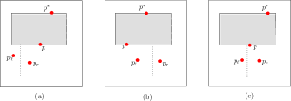
Figure 1: Three different cases while processing a point $p$ in the top-down phase

Without loss of generality, let us assume that $p$ is to the left of $p^{*}$, and $p_{\ell}$ and $p_{r}$ be its two children. Here, three cases may arise: (i) both $p_{\ell}$ and $p_{r}$ are to the left of $p$ (Figure 1(a)), (ii) both $p_{\ell}$ and $p_{r}$ are to the right of $p$ (Figure 1(b)), and (iii) $p_{\ell}$ and $p_{r}$ are in different sides of $p$ (Figure 1(c)). The actions taken in the three different cases are stated below.

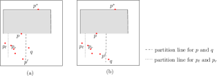
Figure 2: Demonstration of Case (i)

Case (i)

Here, both $p_{\ell}$ and $p_{r}$ are not inserted in $Q_{\ell}$. However, we need to follow the right links starting from $p_{r}$ until (a) a point $p^{\prime}$ is found inside $\cal I$, or (b) the bottom boundary of the floor is reached (i.e. the index of the right child of the current node on the traversal path is greater than the size $n$ of the array $P$). In case (a), surely we have $x(p^{\prime})<x(q)$ where $q$ is the element at the front-end of $Q_{\ell}$. Now, if $y(p^{\prime})>y(q)$, we insert $p^{\prime}$ at the front-end of $Q_{\ell}$ (see Figure 2(a)). But, if $y(p^{\prime})<y(q)$, we ignore $p^{\prime}$, or in other words, do not insert it in $Q_{\ell}$ (see Figure 2(b)).

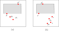
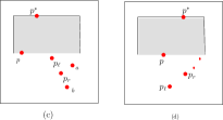
Figure 3: Demonstration of Case (ii)

Case (ii)

Here three different situations may arise: (a) both $p_{\ell}$ and $p_{r}$ are to the left of $p^{*}$, (b) both $p_{\ell}$ and $p_{r}$ are to the right of $p^{*}$, and (c) $p_{\ell}$ and $p_{r}$ are in different sides of $p^{*}$. In subcase (a), if $y(p_{\ell})>y(p_{r})$, we insert $p_{r}$ and $p_{\ell}$ at the front-end of $Q_{\ell}$ in this order (see Figure 3(a)); otherwise only $p_{r}$ is put in $Q_{\ell}$, and $p_{\ell}$ is ignored. In subcase (b), we insert both $p_{r}$ and $p_{\ell}$ at the rear-end of $Q_{r}$. This may need deleting elements of $Q_{r}$ from its rear-end. Such a situation is demonstrated in Figure 3(b). Here $a$ and $b$ are already present in $Q_{r}$; while inserting $p_{r}$, $b$ is deleted from its rear-end since $y(b)<y(p_{r})$. Next, $p_{\ell}$ is also inserted in $Q_{r}$ in the same manner. Note that, while inserting $p_{\ell}$, $p_{r}$ may also be deleted (see Figure 3(c)). In subcase (c), $p_{\ell}$ and $p_{r}$ will need to be inserted in $Q_{\ell}$ and $Q_{r}$ respectively. Note that, if $Q_{\ell}$ is non-empty, then $p_{\ell}$ appears to the left of all the elements present in $Q_{\ell}$. Thus, if $y(p_{\ell})$ is greater than the $y$-coordinate of the element present at the front-end of $Q_{\ell}$, then $p_{\ell}$ is inserted at the front-end of $Q_{\ell}$. Similarly, if there is any element in $Q_{r}$, $p_{r}$ will be left to all of them. Here, $p_{r}$ must be added at the rear-end of $Q_{r}$; if needed, some element of $Q_{r}$ are deleted from its rear-end. The tiny points in Figure 3(d) are already present in the $Q_{r}$. Note that, if this situation arises, at least one of $Q_{\ell}$ and $Q_{r}$ must be empty.

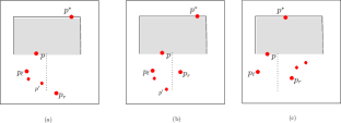
Figure 4: Demonstration of Case (iii)

Case (iii)

Here, first $p_{r}$ is inserted in either at the front-end of $Q_{\ell}$ or at the rear-end of $Q_{r}$ depending on whether $p_{r}$ is to the left or right of $p^{*}$ (see Figure 4). Note that, here $p_{\ell}$ must be ignored. But as in case (i), we need to proceed following the right links starting from $p_{\ell}$ to reach either a point $p^{\prime}$ inside $\cal I$ or the bottom boundary of the floor. If $y(p^{\prime})>y(q)$, where $q$ is at the front-end of $Q_{\ell}$, then $p^{\prime}$ is entered in $Q_{\ell}$ at its front-end (see Figure 4(a)); otherwise $p^{\prime}$ is ignored (see Figure 4(b)). Figure 4(c), shows a situation where $p_{r}$ is to be inserted at the rear-end of $Q_{r}$.

If $p$ has a single child, it is inserted in the queue in a similar manner. If $p$ has no child, no special action needs to be taken; we only proceed to process the next point in the queue.

The similar set of actions are taken for processing the point $p$ when it is at the right side of $p^{*}$. The execution continues until both the queues become empty. Then the last (only one) MER is reported with the resulting curtain $\cal I$ as the horizontal span, and vertical span defined by $p^{*}$ and the bottom boundary of $\cal R$.

4.3 Deletion of the root of $\cal T$

After the completion of a pass, we reorganize the tree $\cal T$ by deleting the point at its root as follows, without computing it afresh.

We start from the root by assigning $i=1$. At each move we consider both the children of $P[i]$, and choose the one, say $P[j]$ having maximum $y$-coordinate. The tie, if arises, is broken arbitrarily. If $P[i]$ has only one child, its index is taken in $j$. We swap $P[i]$ and $P[j]$. and the algorithm proceeds by copying the value of $j$ in $i$. Finally, when no child of $P[i]$ is found, the algorithm terminates. Here the following facts need to be mentioned:

Fact 1

The point at the root is logically deleted, but it still remains in the array $P$. This is essential, since we need to execute a bottom-up phase with all the points in $P$ after the execution of the top-down phase.

Fact 2

Usually, while traversing along a path of $\cal T$, the bottom of the floor $\cal R$ is recognized, when a leaf is reached, or in other words, the index of the child of the said node along the desired direction is greater than the array size $n$. But, such a method may fail from the second pass onwards due to our scheme of deleting the root. Here apart from the usual way, the leaf is also detected if a node (point) is reached whose $y$-coordinate is greater than the $y$-coordinate of the root of $\cal T$.

Fact 3

During the deletion of the root of $\cal T$, when a point is moved from a child node to its parent, it still remains in its own partition according to the partition line defined at that node at the time of creation of the $\cal T$. Thus, binary search property according to the $x$-coordinate values in the present $\cal T$ still remains valid. Moreover, the point having maximum $y$-coordinate in a partition is at the root of its corresponding subtree. Thus the modified $\cal T$ is still a priority search tree.

Fact 4

The tree $\cal T$ may no longer remain balanced after the deletion of some points from $\cal T$. Or in other words, leaf node may appear in different level. However, the length of each search path will still be bounded by $O(\log n)$.

By the virtue of Facts 1, 2, 3, we can execute the subsequent passes to identify all the MERs with top boundary aligned at the point staying at the root node of $\cal T$ in that pass. Fact 4 says that the time required for deletion of root at the end of each pass is $O(\log n)$.

4.4 Complexity Analysis

Lemma 4

A single pass of the top down phase needs $O(\mu+\log n)$ time in the worst case, where $\mu$ is the number of reported answers in that pass.

Proof

In each pass, when an MER is reported, at most two points are inserted in the queue. Thus, the number of points inserted in the queue is at most $2\mu$. Though the insertion of a point in the front-end always takes $O(1)$ time, the insertion of a point in the rear-end may need some deletions prior to that. But, since the total number of deletions in a pass is at most equal to the number of insertions in that pass, and no point is inserted twice in a pass, the time required for a single pass in the top-down phase is $O(\mu)$. The time for the deletion of the root at the end of a pass needs $O(\log n)$ time. Thus, the result follows. ∎

Lemma 5

$|Q_{\ell}|$ and $|Q_{r}|$ can be at most $O(\log n)$ at any instant of time.

Proof

The result follows from the fact that at any instant of time, $Q_{\ell}$ (resp. $Q_{r}$) contains at most two points of a particular level in $\cal T$. We justify this claim assuming the contradiction. Let $\Pi$ ($|\Pi|>2$) be the set of points at the same level of $\cal T$ that are present in $Q_{\ell}$ at an instant of time. Surely, the parents for all of them are not the same, and they are inserted when their parents produced MERs. If we consider the $x$-coordinates of these points as well as their parents, there may exist at most two points (more specifically, the right-most two points) in $\Pi$, say $\pi_{1}$ and $\pi_{2}$, such that $x(\pi_{1})>x(\pi)$ and $x(\pi_{2})>x(\pi)$, where $\pi$ is the right-most one among the already processed parent nodes. Moreover, if such a situation arises, then $\pi_{1}$ and $\pi_{2}$ are the children of $\pi$. Thus, the other points of $\Pi$ have $x$-coordinate less than $x(\pi)$, and hence they can not belong in $Q_{\ell}$. ∎

Theorem 4.1

The time complexity of our algorithm for identifying the maximum area/perimeter axis-parallel rectangle among a set of $n$ points is $O(m+n\log^{2}n)$, and it uses $O(\log n)$ work-space apart from the array $P$ containing input points.

Note: The time complexity of the algorithm can be reduced to $O(m+n\log n)$ if $\cal T$ can be constructed for the first time in $O(n\log n)$ time avoiding the sorting at every level.

5 Finding MER of arbitrary orientation

We now propose an in-place algorithm for finding maximum area empty rectangle of arbitrary orientation among a set of points in $P$. The problem was addressed by Chaudhuri et al. [7]. They introduced the concept of PMER; it is the maximum area empty rectangle of any arbitrary orientation whose four sides are bounded by the members of $P$. It is shown that the number of PMERs is bounded by $O(n^{3})$ in the worst case. It follows from the following observation:

Observation 1

[7] At least one side of a PMER must contain two points from $P$, and other three sides either contain at least one point of $P$ or the boundary of $\cal R$. A corner incident at the boundary of $R$ implies that the corresponding sides contain that boundary point. .

The worst case time complexity of the algorithm proposed in [7] is $O(n^{3})$, and it takes $O(n^{2})$ work-space for executing the algorithm. Our algorithm uses $O(1)$ work-space but its worst case time complexity is $O(n^{3}\log n)$.

5.1 Algorithm

Observation 1 plays the central role in our algorithm. We consider each pair of points $p_{i},p_{j}\in P$, and compute all the PMERs with one boundary passing through $p_{i}$ and $p_{j}$. We assume that the points in $P$ are increasingly ordered with respect to their $x$-coordinates; if tie occurs, then those points are increasingly ordered with respect to their $y$-coordinates. Two variables $i$ and $j$ are used to indicate the pair of points chosen for the processing. We choose different values of $(i,j)$, $i=1,2,\ldots,n-1$ and $j=i+1,i+2,\ldots,n$ in this order. Each time the pair $(i,j)$ is chosen, $p_{i}$ and $p_{j}$ are swapped with $p_{1}$ and $p_{2}$ respectively.

We execute the procedure Process$(p_{i},p_{j})$ to compute all the PMERs with their one boundary passing through $(p_{i},p_{j})$. Note that, after the execution of Process$(p_{i},p_{j})$, the points in $P$ will not be in the increasing order of their coordinates as mentioned above. Thus, in order to choose the next pair for the processing, we need to sort the array $P$ again with respect to their coordinates.

5.1.1 Process$(p_{i},p_{j})$:

Consider the straight line $\ell_{ij}$ passing through $p_{i},p_{j}$. It is truncated by the boundary of $\cal R$ at its two ends. The points $p_{i}$ and $p_{j}$ are assumed to be stored in $P[1]$ and $P[2]$ respectively; the other points are split into two subsets according to the side of $\ell_{ij}$ it belongs. If $P_{1}$ and $P_{2}$ be the sets of points that are below and above $\overline{\ell_{ij}}$ respectively ($|P_{1}|+|P_{2}|=n-2$), then the points in $P_{1}$ are stored in $P[j],j=3,\ldots,|P_{1}|+2$, and the points of $P_{2}$ are stored in $P[j],j=|P_{1}|+3,\ldots,n$. We use the following procedure to partition $P\setminus\{p_{i},p_{j}\}$ into $P_{1}$ and $P_{2}$.

Traverse the array from two directions using two index variables $\alpha$ and $\beta$, initialized to 3 and $n$. The variable $\alpha$ increases until a point in $P_{2}$ is observed; then $\beta$ starts decreasing until a point in $P_{1}$ is observed. Now, $P[\alpha]$ and $P[\beta]$ are swapped. The same process continues until $\alpha\leq\beta$.

We use two scalar locations $n_{1}$ and $n_{2}$ to store $|P_{1}|$ and $|P_{2}|$. We now sort both the set of points $P_{1}$ and $P_{2}$ separately with respect to their distances from $\ell_{ij}$. Note that, the distance values are not stored. While comparing a pair of points, their distance values are computed for the comparison. We now describe the method of computing all the PMERs with the points in $P_{1}$, keeping $(p_{i},p_{j})$ at its top boundary.

As in the earlier algorithm, we consider a curtain whose two sides are bounded by the boundary of $\cal R$, and top boundary is attached to both $p_{i}$ and $p_{j}$. The curtain is allowed to fall. As soon as it hits a point $p\in P_{1}$ it reports a PMER. This point can easily be obtained from the sorted list of $P_{1}$, stored in the array $P$. If the projection $\pi$ of the point $p$ on $\ell_{ij}$ lies inside the interval $[p_{i},p_{j}]$, the processing of $\ell_{ij}$ stops. Otherwise, the curtain is truncated at $\pi$, and the process continues to process the next point in $P_{1}$. After finishing the processing of all the points in $P_{1}$, we process the points in $P_{2}$ in a similar manner to generate the PMERs with their bottom boundary passing through $p_{i}$ and $p_{j}$.

5.2 Correctness and complexity analysis

The correctness of the algorithm follows from the fact that for each pair of points $p_{i},p_{j}\in P$, we have considered all possible PMERs with $(p_{i},p_{j})$ on its one side, and we have considered each pair of points in $P$.

Regarding the time complexity, note that, we have considered $O(n^{2})$ pairs of points. For each pair, we have executed the procedure Process. Each time after the execution of the procedure Process, we need to sort the array $P$ with respect to their $x$ and $y$ coordinates for choosing the next pair of points for processing.

In the procedure Process, the splitting of $P$ into $P_{1}$ and $P_{2}$ needs $O(n)$ time. Sorting the members of $P_{1}$ and $P_{2}$ with respect to their distances from $\ell_{ij}$ needs $O(n\log n)$ time, and then the reporting of the PMERs need $O(n)$ time.

Note that, we have only used four index variables $i$, $j$, $\alpha$ and $\beta$, and two integer locations $n_{1}$ and $n_{2}$ to store size of $P_{1}$ and $P_{2}$. Thus we have the following theorem stating the complexity results of our proposed algorithm.

Theorem 5.1

Given a set of $n$ points, the maximum area/perimeter rectangle of arbitrary orientation can be computed in $O(n^{3}\log n)$ time with $O(1)$ extra space.

References

- [1] A. Aggarwal and S. Suri, Fast algorithm for computing the largest empty rectangle, in Proc. 3rd Annual ACM Symp. on Computational Geometry, pp. 278-290, 1987.
- [2] T. Asano and G. Rote, Constant working-space algorithms for geometric problems, in Proc. 21st. Canadian Conference on Computational Geometry, pp. 87-90, 2009.
- [3] P. Bose, A. Maheshwari, P. Morin, J. Morrison, M. H. M. Smid and J. Vahrenhold, Space-efficient geometric divide-and-conquer algorithms, Computational Geometry- Theory Applications, vol. 37, pp. 209-227, 2007.
- [4] H. Brönnimann, T. M. Chan and E. Y. Chen, Towards in-place geometric algorithms and data structures, in Proc. 20th. Annual ACM Symp. on Computational Geometry, pp. 239-246, 2004.
- [5] H. Brönnimann, J. Iacono, J. Katajainen, P. Morin, J. Morrison and G. T. Toussaint, Space-efficient planar convex hull algorithms, Theoretical Computer Science, vol. 321, pp. 25-40, 2004.
- [6] R. P. Boland and J. Urrutia, Finding the largest axis aligned rectangle in a polygon in time, 13th. Canadian Conference on Computational Geometry, pp. 41-44, 2001.
- [7] J. Chaudhuri, S. C. Nandy and S. Das, Largest empty rectangle among a point set, J. Algorithms, vol. 46, pp. 54-78, 2003.
- [8] E. Y. Chen and T. M. Chan, A space-efficient algorithm for segment intersection, in Proc. 15th. Canadian Conference on Computational Geometry, pp. 68-71, 2003.
- [9] G. Franceschini and V. Geffert, An in-place sorting with comparisons and moves, J. ACM, vol. 52, pp. 515-537, 2005.
- [10] E. M. McCreight, Priority search trees, SIAM J. Comput., vol. 14, pp. 257-276, 1985.
- [11] A. Naamad, D. T. Lee and W. -L. Hsu, On the maximum empty rectangle problem, Discrete Applied Mathematics, vol. 8, pp. 267 - 277, 1984.
- [12] S. C. Nandy, A. Sinha and B. B. Bhattacharya, Location of the largest empty rectangle among arbitrary obstacles, in Proc. 14th. Foundation of Software Technology and Theoretical Computer Science, pp. 159-170, 1994.
- [13] M. Orlowski, A new algorithm for the largest empty rectangle problem, Algorithmica, vol. 5, pp. 65-73, 1990.
- [14] J. Vahrenhold, An in-place algorithm for Klee’s measure problem in two dimensions, Information Processing Letters, vol. 102, pp. 169-174, 2007.