Narrow scope for resolution-limit-free community detection

Abstract

Detecting communities in large networks has drawn much attention over the years. While modularity remains one of the more popular methods of community detection, the so-called resolution limit remains a significant drawback. To overcome this issue, it was recently suggested that instead of comparing the network to a random null model, as is done in modularity, it should be compared to a constant factor. However, it is unclear what is meant exactly by “resolution-limit-free”, that is, not suffering from the resolution limit. Furthermore, the question remains what other methods could be classified as resolution-limit-free. In this paper we suggest a rigorous definition and derive some basic properties of resolution-limit-free methods. More importantly, we are able to prove exactly which class of community detection methods are resolution-limit-free. Furthermore, we analyze which methods are not resolution-limit-free, suggesting there is only a limited scope for resolution-limit-free community detection methods. Finally, we provide such a natural formulation, and show it performs superbly.

I Introduction

The last decade has seen an incredible rise in network studies, and will likely continue to rise Lazer:2009p10015 ; Watts:2007p10016 . Besides the study of properties, such as degree distributions, clustering coefficients and average path length Newman:2003p432 , many complex networks exhibit some modular structure Fortunato:2010p6733 ; Porter:2009p329 . These communities might represent different functions, or sociological communities, and have been successfully studied on a wide variety of networks, ranging from metabolic networks Guimera2005Functional to mobile phone networks Blondel2008Fast and airline transportation networks Guimera2005Worldwide .

One of the most popular methods for community detection is that of modularity Newman2004Finding . The past few years suggestions have been made to extend or alter the original definition, for example, allowing detection in bipartite networks Barber:2007p7162 , networks with negative links Traag:2009p147 , and dynamical networks Mucha:2010p321 . Although modularity optimization seems to be able to accurately identify known community structures Lancichinetti:2008p7072 , it suffers from an inherent problem, namely a resolution limit Fortunato:2007p183 , which affects the effectiveness of community detection Good:2010p10071 . This resolution limit prevents detection of smaller communities in large networks, although this effect can be mitigated somewhat by a so-called resolution parameter kumpala07 , which can be related to time scales of random walks on the network Delvenne:2010p11939 . Another approach adds self-loops in order to circumvent this resolution limit problem Arenas:2008p12974 , and can similarly be related to the random walk approach Delvenne:2010p11939 . The use of such resolution parameters enables the investigation of community structures at various levels of description. The analysis of which levels of description are meaningful or relevant then becomes important, but we will not investigate this issue here.

Recently, a new method has been suggested that would not suffer from this resolution limit Ronhovde:2010p7486 . For showing a method suffers from a resolution limit a few clear cases suffice, but the opposite seems more difficult to argue. That is, although there is no problem for the cases analyzed, perhaps more complex cases will show some issues not yet considered. Hence, a proper definition of resolution-limit-free is called for, which we will develop in this paper. Furthermore, the question then is what methods will suffer from this resolution limit and which not.

We will analyze this question within the framework of the first principle Potts model as developed by Reichardt and Bornholdt Reichardt2007Partitioning . Various methods can be derived from this first principle Potts model, among them modularity, and we will briefly examine them. We will suggest a very simple alternative, which we term the constant Potts model (CPM). It can be easily shown that the CPM is resolution-limit-free according to our definition, but it will follow immediately from the more general theorem we will prove. Arguably, the CPM is the simplest formulation of any (non-trivial) resolution-limit-free method, and can be well interpreted.

In the next section, we will briefly examine this first principle Potts model, review some models that can be derived from it, and introduce the CPM. We will then briefly explain the problem of the resolution limit when using modularity, followed by the introduction of the definition of a resolution-limit-free method (i.e. not suffering from a resolution limit), and we will show some general properties of resolution-limit-free methods. We will then prove which methods are resolution-limit-free and analyze which are not. Finally, we show the CPM method performs superbly.

II Potts Model for Community Detection

First, let us introduce the notation. We consider a connected graph $G=(V,E)$ with $n=|V|$ nodes and $m=|E|$ edges. The adjacency matrix $A_{ij}=1$ if there is an $(ij)$ edge, and $0$ otherwise. For weighted graphs the weight of a link is denoted by $w_{ij}$, while for an unweighted graph we can consider $w_{ij}=1$. We denote the community of a node $i$ by $\sigma_{i}$.

In principle, links within communities should be relatively frequent, while those between communities should be relatively rare. Building on this idea, we will (i) reward links within communities; and (ii) penalize missing links within communities Reichardt2007Partitioning . In general, this can then be written as

$$\mathcal{H}=-\sum_{ij}(a_{ij}A_{ij}-b_{ij}(1-A_{ij}))\delta(\sigma_{i},\sigma_{j}),$$ (1)

where $\delta(\sigma_{i},\sigma_{j})=1$ if $\sigma_{i}=\sigma_{j}$ and zero otherwise, and with some weights $a_{ij},b_{ij}\geq 0$. Minimal $\mathcal{H}$ correspond to desirable partitions, although such a minimum is not necessarily unique. The choice of the weights $a_{ij}$ and $b_{ij}$ are important, and have a definite impact on what type of communities are detected.

II.1 Previous methods

In the current literature, at least four different choices exist (and presumably some other methods may be rewritten as such), leading to four different methods for detecting communities. We will briefly explicate these four different approaches.

Reichardt and Bornholdt (RB) set $a_{ij}=w_{ij}-b_{ij}$ and $b_{ij}=\gamma_{RB}p_{ij}$ with a new variable $p_{ij}$ that represents the probability of a link between $i$ and $j$, known as the random null model. Working out their choice of parameters, we arrive at

$$\mathcal{H}_{RB}=-\sum_{ij}(A_{ij}w_{ij}-\gamma_{RB}p_{ij})\delta(\sigma_{i},\sigma_{j}).$$ (2)

One of the most used null models is the so-called configuration model, which is $p_{ij}=k_{i}k_{j}/2m$, where $k_{i}=\sum_{j}A_{ji}$ is the degree of node $i$. By using this null model, and setting $\gamma_{RB}=1$ we recover the original definition of modularity Newman2004Finding . Independent of the exact choice of the null model $p_{ij}$, it can be shown the method will suffer from a resolution limit kumpala07 , which thereby also holds for modularity Fortunato:2007p183 .

Another approach by Arenas, Fernándes and Gómez (AFG) uses self-loops in order to try to circumvent the resolution limit Arenas:2008p12974 . They do not explicitly derive their model based on the first principle Potts model, but it can easily be done. If we set $a_{ij}=w_{ij}-b_{ij}$ and $b_{ij}=p_{ij}(r)-r\delta(i,j)$, with $p_{ij}(r)=\frac{(k_{i}+r)(k_{i}+r)}{2m+nr}$ and $\delta(i,j)=1$ only if $i=j$ and zero otherwise, we arrive at their model (up to a multiplicative scaling)

$$\mathcal{H}_{AFG}=-\sum_{ij}\left(A_{ij}w_{ij}+r\delta_{ij}-p_{ij}(r)\right)\delta(\sigma_{i},\sigma_{j})$$ (3)

The null model $p_{ij}(r)$ is here defined as the configuration model on the graph where a self-loop with weight $r$ is added to each node.

Ronhovde and Nussinov (RN) do not include any random null model, in order to avoid issues with the resolution limit, and in general set $a_{ij}=w_{ij}$ and $b_{ij}=\gamma_{RN}$ (although for specific networks, such as with negative weights, they allow some minor changes). Working this out we obtain

$$\mathcal{H}_{RN}=-\sum_{ij}(A_{ij}(w_{ij}+\gamma_{RN})-\gamma_{RN})\delta(\sigma_{i},\sigma_{j}).$$ (4)

Finally, the label propagation method Raghavan:2007p11294 can be shown to be equivalent to the Potts model $-\sum_{ij}A_{ij}w_{ij}\delta(\sigma_{i},\sigma_{j})$ Tibely:2008p10903 , which corresponds to the weights $a_{ij}=w_{ij}$ and $b_{ij}=0$. This is the least interesting formulation, since there is only one global optimum, namely all nodes in a single community, which is trivial. However, the local minima could be of some interest.

It is not surprising then that these four different formulations share certain characteristics for some choice of parameters. The RB model is equivalent to the RN model up to a multiplicative constant by using an Erdös-Renyì (ER) null model, i.e. $p_{ij}=p$ and by setting $\gamma_{RN}=\gamma_{RB}p/(1-\gamma_{RB}p)$. For $\gamma_{RN}=0$ the RN model obviously reduces to the label propagation method. Finally, for the AFG model, when using $r=0$ we retrieve the modularity (i.e. the RB model with configuration null model and $\gamma_{RB}=1$).

II.2 Constant Potts model

We introduce an alternative method, that uses slightly different weights. By defining $a_{ij}=w_{ij}-b_{ij}$ and $b_{ij}=\gamma$, we obtain a version that is similar to both the RB and the RN model, but is simpler and more intuitive to work with. If we work this out, we obtain the rather simple expression

$$\mathcal{H}=-\sum_{ij}(A_{ij}w_{ij}-\gamma)\delta(\sigma_{i},\sigma_{j}).$$ (5)

Let us call this the constant Potts model (CPM), with the “constant” here referring to the comparison of $A_{ij}$ to the constant term $\gamma$. It is clear that this is equivalent to the RN model for unweighted graphs by setting $\gamma=\frac{\gamma_{RN}}{1+\gamma_{RN}}$ and ignoring the multiplicative constant. Furthermore, it is equal to the RB model when setting $\gamma=\gamma_{RB}p$ for the ER null model. By setting $\gamma=0$ we retrieve the label propagation method. Also, it is highly similar to an earlier Potts model suggested by Reichardt and Bornholdt Reichardt:2004p11243 .

If we denote the number of edges inside community $c$ by $e_{c}=\sum_{ij}A_{ij}w_{ij}\delta(\sigma_{i},c)\delta(\sigma_{j},c)$, and the number of nodes in community $c$ by $n_{c}=\sum_{i}\delta(\sigma_{i},c)$, we can rewrite Eq. (5) as

$$\mathcal{H}=-\sum_{c}e_{c}-\gamma n^{2}_{c}.$$ (6)

In other words, the model tries to maximize the number of internal edges while at the same time keeping relatively small communities. The parameter $\gamma$ balances these two imperatives. In fact, the parameter $\gamma$ acts as the inner and outer edge density threshold. That is, suppose there is a community $c$ with $e_{c}$ edges and $n_{c}$ nodes. Then it is better to split it into two communities $r$ and $s$ whenever

$$\frac{e_{r\leftrightarrow s}}{2n_{r}n_{s}}<\gamma,$$

where $e_{r\leftrightarrow s}$ is the number of links between community $r$ and $s$. This ratio is exactly the density of links between community $r$ and $s$. So, the link density between communities should be lower than $\gamma$, while the link density within communities should be higher than $\gamma$. This thus provides a clear interpretation of the $\gamma$ parameter.

In general, where $\gamma=\min_{ij}A_{ij}w_{ij}$ the optimal solution is the trivial solution of all nodes in one big community. On the other extreme, when $\gamma=\max_{ij}A_{ij}w_{ij}$, it is optimal to split all nodes in communities, i.e. such that each node forms a community by itself. In fact, communities of one node only exist when $\gamma=\max_{ij}A_{ij}w_{ij}$, since otherwise it will always be beneficial to put the node in one of its neighbors’ communities. Hence, for practical purposes $\min_{ij}A_{ij}w_{ij}\leq\gamma\leq\max_{ij}A_{ij}w_{ij}$.

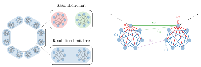
Figure 1: (Color online) The problem of the resolution limit with modularity is usually demonstrated on a ring network of cliques. The cliques are as densely connected as possible, and as sparsely connected between them, while still retaining a connected graph. The resolution limit is said to arise because it will merge cliques depending on the size of the network. In fact, methods that do not suffer from the resolution limit, i.e. resolution-limit-free methods, may merge these cliques also. However, the distinguishing fact between resolution-limit and resolution-limit-free methods is that the first will detect smaller subcommunities when applied to the subgraph (i.e. not the same subpartition), while the latter will not detect smaller subcommunities (i.e. the same subpartition will remain optimal on the subgraph). Of course, whether the communities should consist of only cliques or of multiple joined cliques will still depend on the actual resolution of the method. For CPM this resolution parameter is designated by $\gamma$. So, for a particular value of $\gamma$ the cliques will be separated, while for another value they will be merged. When analyzing the property of resolution-limit-free more in detail, we will investigate this ring of clique network more closely. The actual weights $a_{ij}$ and $b_{ij}$ need to be the same on isomorphic graphs, which restricts the possible number of different weights. We denote these different possibilities with $\alpha$’s for the present links (thicker lines) and $\beta$’s for the missing links (thinner lines). Please refer to the main text for further details.

III Resolution limit

Traditionally the resolution limit is investigated by analyzing the counterintuitive merging of communities Fortunato:2007p183 , for example cliques or some smaller communities that are only sparsely interconnected as displayed in Fig. 1. The RB model with a configuration null model for example will merge two neighboring cliques in this ring network of cliques when kumpala07 $\gamma_{RB}<q/(n_{c}(n_{c}-1)+2)$, where $q$ is the number of cliques and $n_{c}$ is the number of nodes of a clique. Since the number of cliques $q$ is a global variable, it shows modularity might be “hiding” some smaller communities within larger communities, depending on the size of the network. Indeed in Fortunato:2007p183 it was suggested to look at each community to consider whether it had any sub communities. Some different, though related, problems with modularity were noticed in Brandes:2007p196 and more recently in Krings:2011p12227 .

The AFG model considers self-loops of a certain weight to overcome this problem Arenas:2008p12974 . Yet the model still depends on a null model, and so it is not surprising to find that the merging still depends on some global parameters. The implicit inequality for merging two cliques in the ring network of cliques is $q>n_{c}(n_{c}-1)+2+n_{c}r$, which for $\gamma_{RB}=1$ and $r=0$ matches the previous result. Although the resolution parameter $r$ might be used to investigate the community structure at various scales similar to the $\gamma_{RB}$ resolution parameter, it does not fundamentally address the issues of the resolution limit.

The RN model, on the other hand, will only join two cliques when Ronhovde:2010p7486 $\gamma_{RN}<1/(n^{2}_{c}-1)$, which does not depend on the number of cliques $q$, and depends only on the local variable $n_{c}$, so is argued not to suffer from any resolution limit. For the CPM suggested here, we arrive at the condition $\gamma<1/n^{2}_{c}$, which also does not depend on the number of cliques $q$ and can hence also said to be resolution-limit-free. More general, CPM favors to cluster $r$ consecutive cliques instead of $r-1$ at the point when $\gamma<2/(r(r-1)n_{c}^{2})$.

However, it remains somewhat unclear what is meant exactly by resolution-limit-free in the above discussion, and the label resolution-limit-free requires a more precise definition. Consider for example that we take away the dependence on the number of links in the configuration null-model, so that we take $p_{ij}=k_{i}k_{j}$. Notice that this only corresponds to a multiplicative rescaling of $\gamma_{RB}$ by $2m$. Revisiting the case above, we come to the conclusion that cliques are separated whenever $2\gamma_{RB}>(n_{c}(n_{c}-1)+2)^{-2}$, which unsurprisingly no longer depends on any global variables. By the argument employed previously, the method should be resolution-limit-free.

Not all problems have disappeared however. Suppose we take the subgraph consisting of only two of these cliques. We analyze when the method would merge the two cliques in this subgraph, which is the case whenever $2\gamma_{RB}<(n_{c}(n_{c}-1)+1)^{-2}$. Even though neither inequality depends on any global variables, a problem remains. Combining the above two inequalities, we obtain that whenever

$$(n_{c}(n_{c}-1)+2)^{-2}<2\gamma_{RB}<(n_{c}(n_{c}-1)+1)^{-2},$$

the method will separate the cliques in the larger graph, yet merge them in the subgraph.

The above discussion motivates us to consider the following definition of a resolution-limit-free method. The general idea is that when looking at any induced subgraph of the original graph, the partitioning results should not be changed. In order to introduce this definition, let $\mathcal{H}$ be any objective function (which we want to minimize), we then call a partition $\mathcal{C}$ for a graph $\mathcal{H}$-optimal whenever $\mathcal{H}(\mathcal{C})\leq\mathcal{H}(\mathcal{C}^{\prime})$ for any other partition $\mathcal{C}^{\prime}$. We can then define resolution-limit-free as follows.

Definition 1.

Let $\mathcal{C}=\{C_{1},C_{2},\ldots,C_{q}\}$ be a $\mathcal{H}$-optimal partition of a graph $G$. Then the objective function $\mathcal{H}$ is called resolution-limit-free if for each subgraph $H$ induced by $\mathcal{D}\subset\mathcal{C}$, the partition $\mathcal{D}$ is also $\mathcal{H}$-optimal.

Furthermore, we introduce the notion of additive objective functions.

Definition 2.

An objective function $\mathcal{H}$ for a partition $\mathcal{C}=\{C_{1},\ldots,C_{q}\}$ is called additive whenever $\mathcal{H}(\mathcal{C})=\sum_{i}\mathcal{H}(C_{i})$, where $\mathcal{H}(C_{i})$ is the objective function defined on the subgraph $H$ induced by $C_{i}$.

If we have an $\mathcal{H}$-optimal partition $\mathcal{C}$ for an additive resolution-limit-free objective function $\mathcal{H}$, we can replace subpartitions of $\mathcal{C}$ by other optimal subpartitions.

Theorem 1.

Given an additive resolution-limit-free objective function $\mathcal{H}$, let $\mathcal{C}$ be an $\mathcal{H}$-optimal partition of a graph $G$ and let $H\subset G$ be the induced subgraph by $\mathcal{D}\subset\mathcal{C}$. If $\mathcal{D}^{\prime}$ is an alternative optimal partition of $H$ then $\mathcal{C}^{\prime}=\mathcal{C}\setminus\mathcal{D}\cup\mathcal{D}^{\prime}$ is also $\mathcal{H}$-optimal.

Proof.

Define $\mathcal{C}^{\prime}$ and $\mathcal{D}^{\prime}$ as in the theorem. By additivity, $\mathcal{H}(\mathcal{C}^{\prime})=\mathcal{H}(\mathcal{C}\setminus\mathcal{D})+\mathcal{H}(\mathcal{D}^{\prime})$, and by optimality $\mathcal{H}(\mathcal{D}^{\prime})\leq H(\mathcal{D})$. Since also $\mathcal{H}(\mathcal{C})=\mathcal{H}(\mathcal{C}\setminus\mathcal{D})+\mathcal{H}(\mathcal{D})$ we obtain $\mathcal{H}(\mathcal{C}^{\prime})\leq\mathcal{H}(\mathcal{C})$, so $\mathcal{C}^{\prime}$ is also optimal. ∎

Although, this might seem to contradict the NP-hardness of community detection methods, this is not the case. It states that when there are two optimal partitions, any combination of those partitions are optimal, so in a certain sense, they are spanning a space of optimal partitions. It does not say whether such a partition can be easily found. Also, there might be two optimal partitions that cannot be obtained by recombining them, because all communities partly overlap with each other.

It is also possible to prove that a complete graph $K_{n}$ with $n$ nodes is never split (unless into all nodes separately).

Theorem 2.

Given a resolution-limit-free objective function $\mathcal{H}$, the $\mathcal{H}$-optimal partition of $K_{n}$ for all $n$ is either only one community, namely all nodes, or $n$ communities consisting each of one node.

Proof.

Assume on the contrary there is an optimal partition $\mathcal{C}$ of $K_{n}$ such that $1<|\mathcal{C}|<n$. Then for any $\mathcal{D}\subset\mathcal{C}$ the subgraph $H$ induced by $\mathcal{D}$ is a complete graph. But by assumption, $\mathcal{D}$ is then not optimal, and by resolution-limit-free, $\mathcal{C}$ is then not optimal. Hence, inductively, the theorem must hold for all $n$. ∎

Also notice that a resolution-limit-free method will never depend on the size of the network to merge cliques in the ring of cliques network. This can be easily seen from the fact that a subgraph of a large ring of cliques network also appears in a smaller ring. So if the method would merge cliques in some large graph, by the resolution-limit-free property, it would also need to merge them together in the smaller graph. Hence, the actual merging cannot depend on the size of the network. In this sense it captures this prior concept of the resolution limit.

Equipped with this definition, we can analyze the first principle Potts model further. For example, what conditions should be imposed on the weights $a_{ij}$ and $b_{ij}$ in Eq. (1) for the method to be resolution-limit-free? Would a method that takes into account the local number of triangles be resolution-limit-free? Or would it be possible to use the shortest (weighted) path for example?

We can prove that CPM is resolution-limit-free in this sense, just like the RN model and the LP model. The CPM model is also trivially shown to be additive by Eq. (6). Perhaps it is less obvious, but the RB model is not additive, since it cannot be defined in terms of independent contributions, i.e. the contribution $\mathcal{H}(C_{i})$ per community depends on the whole graph $G$, instead of only on the subgraph $H$ induced by $C_{i}$. Nor is the RB model resolution-limit-free according to our definition, regardless of the null model kumpala07 , and hence modularity is not resolution-limit-free. Furthermore, as we have seen, also when using $p_{ij}=k_{i}k_{j}$ the model is not resolution-limit-free. Finally, the AFG model is not resolution-limit-free either.

Since the CPM model is also related to the RB model using the ER null-model, it is tempting to conclude it is also resolution-limit-free. Indeed, this might be said to be the case, if we choose $p$ independently of the graph, i.e. not define it as $p=m/n(n-1)$, and simply choose it as some value $p\in\mathbb{R}$. However, we then obviously retrieve the CPM model. This shows that resolution-limit-free methods are strongly constrained, and there is only a fine line between resolution-limit and resolution-limit-free methods.

This follows from the more general theorem we will now prove. For this, we first introduce the notion of local weights. Again, building on the idea of subgraphs, we define local weights as weights that do not change when looking to subgraphs.

Definition 3.

Let $G$ be a graph, and let $a_{ij}$ and $b_{ij}$ as in Eq. (1) be the associated weights. Let $H$ be a subgraph of $G$ with associated weights $a^{\prime}_{ij}$ and $b^{\prime}_{ij}$. Then the weights are called local if $a_{ij}=\lambda a^{\prime}_{ij}$ and $b_{ij}=\lambda b^{\prime}_{ij}$, where $\lambda=\lambda(H)>0$ can depend on the subgraph $H$.

Clearly then, the RN and CPM model have local weights, while the RB and AFG model do not. This definition says that local weights should be independent of the graph $G$ in a certain sense. In fact, it is quite a strong requirement, as it should even hold for a single link $(ij)$ in the subgraph where only $i$ and $j$ are included. That means it can not depend on any other link but the very link itself. Since for missing links, there is (usually) no associated weight or anything, it can only be constant. There are some exceptions, such as multipartite networks, or networks embedded in geographical space Expert:2011p12973 ; Lambiotte:2008p2987 , where some sensible non-constant local weights can be provided. Hence, the RN model and the CPM model are one of the few sensible options available for having local variables. We can now prove the more general statement that methods using local weights are resolution-limit-free.

Theorem 3.

The objective function $\mathcal{H}$ as defined in Eq. (1) is resolution-limit-free if it has local weights.

Proof.

Let $\mathcal{C}$ be the optimal partition for $G$ with community assignments $c_{i}$, $\mathcal{D}\subset\mathcal{C}$ a subset of this partition, and $H$ the subgraph induced by $\mathcal{D}$ with $h$ nodes. Furthermore, we denote by $d_{i}$ the community indices of $\mathcal{D}$, such that $d_{i}=c_{i}$ for $1\leq i\leq h$ and by $A^{\prime}$ the adjacency matrix of $H$, so that $A_{ij}=A^{\prime}_{ij}$ for $1\leq i\leq h$. Assume $\mathcal{D}$ is not optimal for $H$, and that $\mathcal{D}^{*}$ is optimal, such that $\mathcal{H}(\mathcal{D})>\mathcal{H}(\mathcal{D}^{*})$. Then define $c^{*}$ by setting $c^{*}_{i}=d^{*}_{i}$ for $1\leq i\leq h$ and $c^{*}_{i}=c_{i}$ for $h<i\leq n$. Then because the result is unchanged for the nodes $h<i\leq n$, we have that

$$\Delta\mathcal{H}=\mathcal{H}(\mathcal{C})-\mathcal{H}(\mathcal{C}^{*})=\frac{1}{\lambda}(\mathcal{H}(\mathcal{D})-\mathcal{H}(\mathcal{D}^{*}))>0$$

where the last step follows from the locality of the weights $a_{ij}$ and $b_{ij}$. This inequality contradicts the optimality of $\mathcal{C}$. Hence, for all induced subgraphs $H$, the partition $\mathcal{D}$ is optimal, and the objective function $\mathcal{H}$ is resolution-limit-free. ∎

The converse is unfortunately not true. Consider a graph $G$ with some weights $a_{ij}$ and $b_{ij}$. Then pick a subgraph $H$ induced by some subpartition $\mathcal{D}$, and define the weights $a^{\prime}_{ij}=a_{ij}$ and $b^{\prime}_{ij}=b_{ij}$ except for one particular edge $(kl)$, for which we set $a^{\prime}_{kl}=a_{kl}+\epsilon$. Then for some $\epsilon>0$, the original subpartition will remain optimal in $H$, while the weights are not local. Since the small change of the weight is only made when considering the graph $H$, all other subpartitions will always remain optimal. Of course, such a definition of the weight is rather odd, so in practice we will never use it.

Even though the converse is not true, we can say a bit more. The weights can be a bit different indeed, but there is not that much room for these differences. We demonstrate this on the ring network of cliques. The weights can depend only on the graph, so if $G$ and $G^{\prime}$ are two isomorphic graphs, then $a_{ij}(G)=a_{i^{\prime}j^{\prime}}(G^{\prime})$, where $i$ and $i^{\prime}$ are two isomorphic nodes. Hence, only a number of weights can be different from each other in the ring network, as illustrated in Fig. 1. All nodes within a clique are isomorphic, except the node that connects to other cliques. So, all the edges among those $n_{c}-1$ nodes are similar, and will have the same weight $\alpha_{1}$. All edges from these $n_{c}-1$ nodes to the “outside” node will have the same weight $\alpha_{2}$. Finally, the edge connecting two cliques is denoted by $\alpha_{3}$. The missing self-loop for the special outside node is denote by $\beta_{2}$ while the missing self-loop for the other nodes in the cliques is denoted by $\beta_{1}$. Finally, there is (1) a missing link between the outside node and a normal node denoted by $\beta_{3}$; and (2) a missing link between two normal nodes, denoted by $\beta_{4}$. These weights are illustrated in Fig. 1.

Let us now analyze when the method will not be resolution-limit-free. Then, the cliques must be merged in some (large) graph, while for the subgraph consisting of these two merged cliques, they should be separated by the method. Or conversely, they should be separated in some (large) graph, but merged in the subgraph. We can write the $\mathcal{H}_{s}$ for all $q$ cliques being separate as

$$\mathcal{H}_{s}=-q({\color[rgb]{0.215686,0.494118,0.721569}\alpha_{1}(n_{c}-1)(n_{c}-2)}+{\color[rgb]{0.894118,0.101961,0.109804}2\alpha_{2}(n_{c}-1)}\\ -{\color[rgb]{0.215686,0.494118,0.721569}(n_{c}-1)\beta_{1}}-{\color[rgb]{0.894118,0.101961,0.109804}\beta_{2}})$$

and $\mathcal{H}_{m}$ for merging all two consecutive cliques as

$$\mathcal{H}_{m}=-\frac{q}{2}2({\color[rgb]{0.215686,0.494118,0.721569}\alpha_{1}(n_{c}-1)(n_{c}-2)}+{\color[rgb]{0.894118,0.101961,0.109804}2\alpha_{2}(n_{c}-1)}\\ -{\color[rgb]{0.215686,0.494118,0.721569}(n_{c}-1)\beta_{1}}-{\color[rgb]{0.894118,0.101961,0.109804}\beta_{2}}+{\color[rgb]{0.301961,0.686275,0.290196}\alpha_{3}}-{\color[rgb]{0.301961,0.686275,0.290196}\beta_{3}(n_{c}-1)}-{\color[rgb]{0.596078,0.305882,0.639216}\beta_{4}(n_{c}-1)^{2}})$$

Furthermore, for the induced subgraph $H$ consisting of two consecutive cliques, we can write $\mathcal{H}^{\prime}_{s}$ for separating the two cliques and $\mathcal{H}^{\prime}_{m}$ for merging them, similarly as before, where $\alpha^{\prime}$ and $\beta^{\prime}$ are the weights for the subgraph $H$. Then the method is not resolution-limit-free if it would merge the two cliques at a higher level (i.e. when $\mathcal{H}_{m}<\mathcal{H}_{s}$) yet would not merge them at smaller scale (i.e. when $\mathcal{H}^{\prime}_{s}<\mathcal{H}^{\prime}_{m}$), or vice versa. Working out this condition for $\mathcal{H}_{m}<\mathcal{H}_{s}$ (and similarly for $\mathcal{H}_{m}>\mathcal{H}_{s}$) gives us

$${\color[rgb]{0.301961,0.686275,0.290196}\alpha_{3}}>(n_{c}-1)({\color[rgb]{0.596078,0.305882,0.639216}\beta_{4}(n_{c}-1)}+{\color[rgb]{0.301961,0.686275,0.290196}\beta_{3}}),$$

while for $\mathcal{H}^{\prime}_{s}<\mathcal{H}^{\prime}_{m}$ (and similarly for $\mathcal{H}^{\prime}_{s}>\mathcal{H}^{\prime}_{m}$) we obtain

$${\color[rgb]{0.301961,0.686275,0.290196}\alpha^{\prime}_{3}}<(n_{c}-1)({\color[rgb]{0.596078,0.305882,0.639216}\beta^{\prime}_{4}(n_{c}-1)}+{\color[rgb]{0.301961,0.686275,0.290196}\beta^{\prime}_{3}}).$$

Combining these two inequalities for both cases we obtain

$${\color[rgb]{0.301961,0.686275,0.290196}\alpha^{\prime}_{3}}({\color[rgb]{0.596078,0.305882,0.639216}\beta_{4}(n_{c}-1)}+{\color[rgb]{0.301961,0.686275,0.290196}\beta_{3}}) <{\color[rgb]{0.301961,0.686275,0.290196}\alpha_{3}}({\color[rgb]{0.596078,0.305882,0.639216}\beta^{\prime}_{4}(n_{c}-1)}+{\color[rgb]{0.301961,0.686275,0.290196}\beta^{\prime}_{3}}),$$ (7)

$${\color[rgb]{0.301961,0.686275,0.290196}\alpha^{\prime}_{3}}({\color[rgb]{0.596078,0.305882,0.639216}\beta_{4}(n_{c}-1)}+{\color[rgb]{0.301961,0.686275,0.290196}\beta_{3}}) >{\color[rgb]{0.301961,0.686275,0.290196}\alpha_{3}}({\color[rgb]{0.596078,0.305882,0.639216}\beta^{\prime}_{4}(n_{c}-1)}+{\color[rgb]{0.301961,0.686275,0.290196}\beta^{\prime}_{3}}).$$ (8)

where either Eq. (7) or (8) should hold. Hence, only if the left hand side equals the right hand side, it does not constitute a counter example. Working out this equality, there are two possibilities. Either the weights should be local, or the following equality should hold

$$n_{c}-1=\frac{{\color[rgb]{0.301961,0.686275,0.290196}\alpha_{3}}{\color[rgb]{0.596078,0.305882,0.639216}\beta^{\prime}_{3}}-{\color[rgb]{0.301961,0.686275,0.290196}\alpha^{\prime}_{3}}{\color[rgb]{0.596078,0.305882,0.639216}\beta_{3}}}{{\color[rgb]{0.301961,0.686275,0.290196}\alpha^{\prime}_{3}}{\color[rgb]{0.596078,0.305882,0.639216}\beta_{4}}-{\color[rgb]{0.301961,0.686275,0.290196}\alpha_{3}}{\color[rgb]{0.596078,0.305882,0.639216}\beta^{\prime}_{4}}}.$$

Obviously, this again constitutes some very particular case of non-local weights. We can repeat this same procedure for other subpartitions, and for other graphs, thereby forcing the weights to be of a very particular kind. This thus leaves little room for having any sensible non-local definition such that the method is resolution-limit-free.

This means resolution-limit-free community detection has only a quite limited scope. In fact, the CPM seems to be the simplest non-trivial sensible formulation of any general resolution-limit-free method, although there is some leeway for special graphs (i.e. having some node properties, such as multipartite graphs). This is not to say that methods with non-local weights (e.g. modularity, AFG, number of triangles, shortest path, betweenness) should never be used for community detection at all, they are just never resolution-limit-free.

IV Performance

In order to assess the performance of the proposed CPM model, we performed various tests. Using the latest suggested test networks Lancichinetti:2008p7072 we find that the CPM model and the accompanying algorithm is both very accurate and efficient. More details on the efficient Louvain-like algorithm, the test procedure and the calculations on the resolution parameters can be found in the appendix at the end of this article.

We have examined both directed test networks as well as hierarchical test networks, where communities exist at multiple levels in the data. Communities become less discernible for higher values of the parameter $\mu$ of having links outside its community. For hierarchical communities, there are two such parameters: $\mu_{1}$ for the first level (the large communities), and $\mu_{2}$ for the second level (the subcommunities). These mixing parameters allow us to calculate what the inner and outer densities of communities are. We exploit this fact to calculate the proper $\gamma=\gamma^{*}$ in order to investigate the performance of the CPM, and similarly $\gamma_{RB}=\gamma^{*}_{RB}$ for the RB model using the configuration null model. This way, the results do not depend on any particular method to determine the correct parameter, which represents another challenging problem.

Some of the earlier algorithms and models that showed excellent performance Lancichinetti:2009p7112 are the Louvain Blondel2008Fast method for optimizing modularity, and the Infomap method Rosvall2007Informationtheoretic . In Fig. 2 we have displayed the results for (1) the CPM model; (2) the RB model using an ER null model (i.e. CPM with $\gamma=p$); (3) the RB model using the configuration null model with “corrected” parameter value $\gamma_{RB}^{*}$; (4) the modularity model, (i.e. RB using the configuration null model and $\gamma_{RB}=1$); and finally (5) the Infomap method. We have performed tests on networks having $n=10^{3}$ and $n=10^{4}$ nodes, with a degree distribution exponent of $2$ (with average degree $15$ and maximum degree $50$) and community size distribution exponent $1$ (with community sizes ranging from $20$ to $100$). Per value of $\mu$ 100 graphs were used to obtain this result.

It can be clearly seen that CPM performs extremely well. The difference in performance of the CPM model in comparison to the RB model using the ER null model is especially striking. This is not a consequence of the method being resolution-limit-free or not, but it rather depends on choosing the correct resolution parameter. Obviously then, setting $\gamma=p$ is in general not a very good strategy, and for general networks one should carefully analyze at which resolution the network contains meaningful partitions.

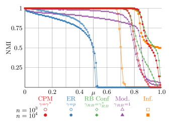
Figure 2: (Color online) Performance of various community detection methods in terms of Normalized Mutual Information (NMI) depending on mixing parameter $\mu$. Results are shown for (1) CPM, using the calculated resolution parameter $\gamma^{*}$; (2) the RB model with an ER random null model (i.e. corresponding to CPM using $\gamma=p$); (3) the RB model with a configuration null model with a calculated resolution parameter $\gamma_{RB}^{*}$; (4) modularity, in other words, the RB model with a configuration model using $\gamma_{RB}=1$; and finally (5) the Infomap method. The open symbols denote results for $n=10^{3}$ and the closed symbols for $n=10^{4}$.

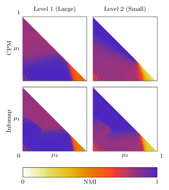
Figure 3: (Color online) Performance of CPM and Infomap on a hierarchical benchmark network in terms of Normalized Mutual Information (NMI) depending on mixing parameters $\mu_{1}$ and $\mu_{2}$. The networks had $n=10^{4}$ nodes with a degree distribution exponent of $2$ (with average degree $20$ and maximum degree $50$) and community size distribution exponent $1$ for both small (size ranging from $10$ to $50$) and large communities (size ranging from $50$ to $300$). Per combination of parameters 10 graphs were used to obtain this result. The resolution parameters $\gamma$ for the two different levels were calculated analytically for CPM.

A similar effect also shows for modularity (or the RB model using the configuration model), such that when $\gamma_{RB}$ is chosen appropriately (i.e. using $\gamma_{RB}=\gamma_{RB}^{*}$) the method will perform better than at the ordinary resolution $\gamma_{RB}=1$. Indeed, the results of the CPM model and the RB model using the configuration null model using $\gamma^{*}_{RB}$ are rather comparable, although the latter’s performance drops less quickly, and then outperforms CPM. Interestingly, when we use the ordinary resolution $\gamma_{RB}=1$, it becomes more difficult to detect communities in large networks using the configuration model. This constrasts with the results when we choose the appropriate resolution parameter $\gamma^{*}$, $\gamma_{RB}^{*}$ and indeed also for the Infomap method. Indeed it can be shown that the communities should become more clearly discernible for larger networks when the community sizes remain similar.

Surprisingly, both methods outperform the Infomap method, which performed superbly in previous tests Lancichinetti:2009p7112 , when the appropriate resolution parameter is chosen. This show that determining the correct or meaningful resolution is an important issue. This remains a challenging problem, and various methods have been proposed to do so Fortunato:2010p6733 , for example by looking at the stability of multiple (randomized) runs of an algorithm Lambiotte:2010p6743 ; Ronhovde:2010p7486 , by looking for large ranges of the parameter over which the results remain stable Arenas:2008p12974 , investigating the stability when the network is slightly perturbed Gfeller:2005p13024 or by looking at how significant the partition is compared to a graph ensemble Bianconi:2009p13095 .

We have also performed extensive tests on hierarchical networks, where the method also performs well, and is able to extract the two different levels of communities effectively, as displayed in Fig. 3. For relatively low $\mu_{2}\lessapprox 0.7$, the first (larger) level becomes more clear for low $\mu_{1}$, while the second (smaller) level becomes more clear for larger $\mu_{1}$. This is both the case for a recent hierarchical version of the Infomap method Rosvall:2011p11938 and the CPM method. The Infomap method seems to be slightly better at detecting the correct communities, but the CPM method remains highly competitive. The possibility for having various scales of description of the network seems important, as many networks seem to have at least some hierarchical structure.

V Conclusion

Several community detection methods, among which modularity, are affected by the problem of the resolution limit. In this paper we have provided a novel rigorous definition of what it means for a community detection method to be resolution (limit) free. Most importantly, we are able to prove exactly which community detection methods are resolution-limit-free, namely those methods that use local weights. This also clarifies the relationship between local methods and the resolution limit. However, we do not address the issue of determining an actual meaningful resolution, which remains a challening problem.

Moreover, there does not seem to be much room for having resolution-limit-free methods without local weights. Of the few possibilities available for having resolution-limit-free community detection, the constant Potts Model (CPM) we introduced in this paper seems to be the simplest possible formulation, and performs excellent. A rigorous definition of resolution-limit-free community detection allows for a more articulate analysis, and induces further progress on developing novel and meaningful methods.

Appendix A Louvain like Algorithm

The algorithm we employ is derived from the Louvain method Blondel2008Fast . We use the concept of node size, denoted by $n_{i}$ for a node $i$, initialized to $n_{i}=1$ (indeed the community size $n_{c}=\sum_{i}n_{i}\delta(\sigma_{i},c)$ is related). We first iterate (randomly) over all nodes, and put nodes greedily into the community that minimizes Eq. (5). We subsequently create a new graph based on the communities, and new node sizes, and reiterate over this new smaller graph. More specifically:

1. Initialize $A_{ij}=w_{ij}$, with $w_{ij}=1$ in the case of unweighted networks, and set $n_{i}=1$ for all nodes $i$.

2. Loop over nodes $i$, remove it from its community and calculate for each community $c$ the increase if we would put node $i$ into community $c$,

   $$\Delta\mathcal{H}(\sigma_{i}=c)=-(e_{i\leftrightarrow c}-2\gamma n_{i}\sum_{j}n_{j}\delta(\sigma_{j},c)),$$ (9)

   where $e_{i\leftrightarrow c}=\sum_{j}(A_{ij}+A_{ji})\delta(\sigma_{j},c)$ is the number of edges between node $i$ and community $c$. We put node $i$ into the community $c$ for which $\Delta\mathcal{H}(\sigma_{i}=c)$ is minimal. We iterate until we can no longer decrease the objective function.

3. We build a new graph $A^{\prime}_{cd}\allowbreak=\sum_{ij}A_{ij}\delta(\sigma_{i},c)\delta(\sigma_{j},d)$ and node sizes $n^{\prime}_{c}=\sum_{i}n_{i}\delta(\sigma_{i},c)$. We repeat step 9 by setting $A=A^{\prime}$ and $n=n^{\prime}$ until the objective function can no longer be decreased.

The implementation of the algorithm in C++ can be downloaded from the author’s website: http://perso.uclouvain.be/vincent.traag.

Notice that for resolution-limit-free methods, the results should be unchanged on subgraphs. Hence, we could therefore perform the method recursively on subgraphs. We suggest then the following improvement. First we cut the network at each recursive call, until the density of the subgraph exceeds $\gamma$. Then, we recombine the subgraphs, and loop over nodes/communities to find improvements until we can no longer increase greedily, and return to the previous recursive function call. These calls should be easily parallelized, making community detection in even larger graphs or in an on-line setting possible by using cluster computing.

Appendix B Benchmark tests

The benchmark networks are created using a known community structure, i.e. a planted community structure. The community sizes $n_{c}$ are chosen from a distribution following a power-law $\Pr(n_{c}=n)\sim n^{-\tau_{2}}$. The degrees $k_{i}$ of the nodes are also chosen from a power-law distribution $\Pr(k_{i}=k)\sim k^{-\tau_{1}}$. The stubs are then connected, with probability $1-\mu$ within a community, and with probability $\mu$ between two communities. A lower bound $\underline{n_{c}}$ and upper bound $\overline{n_{c}}$ on the community sizes is imposed, while for the degree the average degree $\langle k\rangle$ is specified. For the hierarchical version, there are two levels, with the communities of the second level embedded in the first level. A fraction of $\mu_{1}$ of the links is placed between two different macro communities at the first level, while a fraction of $\mu_{2}$ of the links are placed between the small communities of the second level (but within the same large community).

Instead of detecting the resolution algorithmically, we calculate the proper resolution parameter value $\gamma$ analytically (and therefore, beforehand). In order to do so, we consider the following. The resolution parameter $\gamma$ acts as a sort of threshold on inner and outer community density. If we were to set $\gamma$ equal to the inner density, it would be rather difficult to fulfill the condition that the inner density should be higher than that, and similarly so for $\gamma$ equal to the outer density. So, we need to be as far as possible from both the inner density as well as the outer density, which would be simply the average of the two.

The inner density for a community having $n_{c}$ nodes can be easily found as

$$p_{in}=\frac{(1-\mu)\langle k\rangle}{n_{c}-1},$$ (10)

and the outer density (i.e. all the edges originating from a community to the outside) is

$$p_{out}=\frac{\mu\langle k\rangle}{n-n_{c}},$$ (11)

where $n$ is simply the total number of nodes. The average community size $\langle n_{c}\rangle$, which is proportional to

$$\langle n_{c}\rangle\sim\sum_{n=\underline{n_{c}}}^{\overline{n_{c}}}nn^{-\beta},$$ (12)

where $\underline{n_{c}}$ is the minimal community size and $\overline{n_{c}}$ the maximal community size, than gives us the $\langle p_{in}\rangle$ and $\langle p_{out}\rangle$ for the average community size. The best resolution parameter is then $\gamma^{*}=\frac{1}{2}(\langle p_{in}\rangle+\langle p_{out}\rangle)$.

For the hierarchical test networks, we can perform a similar analysis, and use the average of the inner and outer density, similar as before, for the two different levels. Ordinarily, the communities are assumed to exist whenever $p_{in}>p_{out}$.

For modularity, we can also calculate similar bounds. When we define by $e_{c}$ the number of edges within community $c$ and by $[e_{c}]$ the number of expected edges within a community, modularity can be written as

$$\mathcal{H}=-\sum_{c}e_{c}-\gamma_{RB}[e_{c}].$$ (13)

Hence, each community should have a “expected density” or “degree density” $\tilde{p}_{in}=e_{c}/[e_{c}]$ within communities lower than $\gamma$, while the outer degree density should be lower between communities. Writing this out in terms of the configuration model, given the model of the test networks, we arrive at

$$\tilde{p}_{in} =\frac{(1-\mu)n}{n_{c}},$$ (14)

$$\tilde{p}_{out} =\frac{\mu n}{n-n_{c}}.$$ (15)

These degree densities lack a clear interpretation, in contrast with CPM. Similar as before we simply set $\gamma^{*}_{RB}=\frac{1}{2}(\langle\tilde{p}_{in}\rangle+\langle\tilde{p}_{out}\rangle)$ for the average community size $\langle n_{c}\rangle$.

For comparing our results to the known community structure, we use the normalized mutual information. Given two different partitions $C$ and $D$, the mutual information $I$ is defined as

$$I(C,D)=-\sum_{r,s}\frac{n_{r,s}}{n}\log n\frac{n_{r,s}}{n_{r}n_{s}}$$

with $n_{r,s}$ being the number of nodes that are in community $r$ in partition $C$ and in community $s$ in partition $D$, while $n_{r}$ simply denotes the number of nodes in community $r$. The normalized mutual information $I_{n}(C,D)$ is then defined as

$$I_{n}(C,D)=\frac{2I(C,D)}{H(C)+H(D)},$$

where $H(C)$ indicates the entropy of a partition $C$, which is defined as

$$H(C)=-\sum_{c}\frac{n_{c}}{n}\log\frac{n_{c}}{n}.$$

The normalized mutual information $0\leq I_{n}(C,D)\leq 1$, with $1$ indicating equivalent partitions.

References

- (1) D. Lazer, A. S. Pentland, L. Adamic, S. Aral, A. L. Barabasi, D. Brewer, N. Christakis, N. Contractor, J. Fowler, M. Gutmann, T. Jebara, G. King, M. Macy, D. Roy, and M. V. Alstyne, Science 323, 721 (Feb 2009)
- (2) D. J. Watts, Nature 445, 489 (Jan 2007)
- (3) M. E. J. Newman, SIAM Rev 45, 167 (2003)
- (4) S. Fortunato, Phys Rep 486, 75 (Feb 2010)
- (5) M. A. Porter, J.-P. Onnela, and P. J. Mucha, Not Am Math Soc 56, 1082 (Jan 2009)
- (6) R. Guimerà and L. A. N. Amaral, Nature 433, 895 (Feb 2005)
- (7) V. D. Blondel, J.-L. Guillaume, R. Lambiotte, and E. Lefebvre, J Stat Mech-Theory E 2008, P10008 (Oct 2008)
- (8) R. Guimerà, S. Mossa, A. Turtschi, and L. Amaral, Proc Natl Acad Sci USA 102, 7794 (May 2005)
- (9) M. E. J. Newman and M. Girvan, Phys Rev E 69, 026113 (Feb 2004)
- (10) M. J. Barber, Phys Rev E 76, 066102 (Dec 2007)
- (11) V. A. Traag and J. Bruggeman, Phys Rev E 80, 036115 (Sep 2009)
- (12) P. J. Mucha, T. Richardson, K. Macon, M. A. Porter, and J.-P. Onnela, Science 328, 876 (May 2010)
- (13) A. Lancichinetti, S. Fortunato, and F. Radicchi, Phys Rev E 78, 046110 (Oct 2008)
- (14) S. Fortunato and M. Barthelemy, Proc Natl Acad Sci USA 104, 36 (Jan 2007)
- (15) B. H. Good, Y.-A. de Montjoye, and A. Clauset, Phys Rev E 81, 046106 (Apr 2010)
- (16) J. M. Kumpula, J. Saramäki, K. Kaski, and J. Kertész, Eur Phys J B 56, 41 (Mar 2007)
- (17) J.-C. Delvenne, S. Yaliraki, and M. Barahona, Proc Natl Acad Sci USA 107, 12755 (Jul 2010)
- (18) A. Arenas, A. Fernández, and S. Gómez, New J Phys 10, 053039 (May 2008)
- (19) P. Ronhovde and Z. Nussinov, Phys Rev E 81, 046114 (Jan 2010)
- (20) J. Reichardt and S. Bornholdt, Phys Rev E 76, 015102+ (2007)
- (21) U. N. Raghavan, R. Albert, and S. Kumara, Phys Rev E 76, 036106 (Sep 2007)
- (22) G. Tibely and J. Kertész, Physica A 387, 4982 (Aug 2008)
- (23) J. Reichardt and S. Bornholdt, Phys Rev Lett 93, 218701 (Nov 2004)
- (24) U. Brandes, D. Delling, M. Gaertler, R. Görke, M. Hoefer, Z. Nikoloski, and D. Wagner, Lect Notes Comput Sc 4769, 121 (Jan 2007)
- (25) G. Krings and V. D. Blondel, Arxiv preprint arXiv:1103.5569(Jan 2011)
- (26) P. Expert, T. Evans, V. D. Blondel, and R. Lambiotte, Proc Natl Acad Sci USA 108, 7663 (Jan 2011)
- (27) R. Lambiotte, V. Blondel, C. Dekerchove, E. Huens, C. Prieur, Z. Smoreda, and P. van Dooren, Physica A 387, 5317 (Sep 2008)
- (28) A. Lancichinetti and S. Fortunato, Phys Rev E 80, 056117 (Nov 2009)
- (29) M. Rosvall and C. T. Bergstrom, Proc Natl Acad Sci USA 104, 7327 (May 2007)
- (30) E. A. Leicht and M. E. J. Newman, Phys Rev Lett 100, 118703+ (2008)
- (31) R. Lambiotte, Arxiv preprint arXiv:1004.4268(Jan 2010)
- (32) D. Gfeller, J.-C. Chappelier, and P. de Los Rios, Phys Rev E 72, 056135 (Nov 2005)
- (33) G. Bianconi, P. Pin, and M. Marsili, Proc Natl Acad Sci USA 106, 11433 (Jul 2009)
- (34) M. Rosvall and C. T. Bergstrom, PloS one 6, e18209 (Jan 2011)