Entanglement Sudden Death and Sudden Birth in Semiconductor Microcavities

Abstract

We explore the dynamics of the entanglement in a semiconductor cavity QED containing a quantum well. We show the presence of sudden birth and sudden death for some particular sets of the system parameters.

I Introduction

Entanglement as the central feature of quantum mechanics distinguishes a quantum system from its classical counterpart. As an important physical resource, it has many applications in quantum information theory. Among the well known applications of entanglement are superdense coding abeye , quantum state teleportationbenn ; agrawal . Efforts to quantify this resource are often termed entanglement theoryplenio . Quantum entanglement also has many different applications in the emerging technologies of quantum computing and quantum cryptography zuko ; nnrr , and has been used to realize quantum teleportation experimentallyxian .
Quantum entanglement has attracted a lot of attention in recent years in various kinds of quantum optical systems yonac ; Lajos ; chan ; barrada1 ; barrada2 ; barrada3 .

Several methods to quantify entanglement have been proposed. For pure states, the partial entropy of the density matrix can provide a good measure of entanglement. Information entropies are also used to quantify the entanglement in quantum information shann . In this regard the von Neumann Entropy (NE) neum , Linear Entropy (LE) and Shannon information Entropy (SE) have been frequently used in treating entanglement in the quantum systems. It is worth mentioning that the SE involves only the diagonal elements of the density matrix and in some cases gives information similar to that obtained from the NE and LE. On the other hand, there is an additional entropy, namely, the Field Wehrl Entropy (FWE) wehrl . This measure has been successfully applied in description of different properties of the quantum optical fields such as phase-space uncertainty abotalb09 ; mira1 , decoherence orl ; deco etc.

The FWE is more sensitive in distinguishing states than the NE since FWE is a state dependent mira3 . The concept of the Wehrl Phase Distribution (WPD) has been developed and shown that it serves as a measure of both noise (phase-space uncertainty) and phase randomization mira3 . Furthermore, the FWE has been applied to the dynamical systems. In this respect the time evolution of the FWE for the Kerr-like medium has been discussed in jex . For the Jaynes-Cumming model the FWE gives an information on the splitting of the Q-function in the course of the collapse region of the atomic inversion as well as on the atomic inversion itself orl ; obad ; abotalb07 .
In the current contribution we study the evolution behavior of entanglements in a semiconductor cavity QED containing a quantum well coupled to the environment by the FWE, generalized concurrence vector and WPD. We also explore the situation in which the entanglement decays to zero abruptly. Recently, Yu and Eberly yu1 ; yu12 ; yu2 ; yu3 ; yu4 showed that entanglement loss occurs in a finite time under the action of pure vacuum noise in a bipartite state of qubits. They found that, even though it takes infinite time to complete decoherence locally, the global entanglement may be lost in finite time. This phenomenon of sudden loss of entanglement has been named as ”entanglement sudden death” (ESD). . Opposite to the currently extensively discussed ESD, Entanglement Sudden Birth (ESB)yona ; lop is the creation of entanglement where the initially unentangled qubits can be entangled after a finite evolution time. These phenomena have recently received a lot of attention in cavity-QED and spin chainshan ; man , and have been observed Exprimentallydav1 ; dav2 .
The paper is organized as follows; Section 2 displays the physical system and its model Hamiltonian. Section 3 devotes to evolution equations of the system by the quantum trajectory approaching. Section 4 discusses the entanglement due to Wehrl entropy, generalized concurrence and the Wehrl phase distribution and section 5 supplies a conclusion and outlooks.

II Model

The considered system is a quantum well confined in a semiconductor microcavity. The semiconductor microcavity is made of a set of Bragg mirrors with specific separation taken to be of the order of the wavelength $\lambda$. In the system under consideration, we restricted our discussion to the interaction of electromagnetic field with two bands in the weak pumping regime. The electromagnetic field can make an electron transition from valance to conduction band. This transition simultaneously creates a single hole in the valance band which leads to generation of exciton in the system. One can use an effective Hamiltonian without spin effects for describing the exciton-photon coupling in the cavity as 28 ; 29 ; 30 ; 31 ; 32 ; 33 ; 34 ; 35 :

$$H = \hbar\omega_{p}a^{{\dagger}}a+\hbar\omega_{e}b^{{\dagger}}b+\imath\hbar g^{\prime}(a^{{\dagger}}b-b^{{\dagger}}a)$$ (1)

$$+ \hbar\alpha^{\prime}b^{{\dagger}}b^{{\dagger}}bb+\imath\hbar(\varepsilon^{\prime}e^{\imath\omega t}a^{{\dagger}}-h.c)+H_{r},$$

where $\omega_{p}$ and $\omega_{e}$ are the frequencies of the photonic and excitonic modes of the cavity respectively. The bosonic operators a and b are respectively describing the photonic and excitonic annihilation operators and verifying $[a,a^{{\dagger}}]=1;[b,b^{{\dagger}}]=1$. The first two terms of the Hamiltonian describe respectively the energies of photon and exciton. The third term corresponds to the photon-exciton coupling with a constant of coupling $g^{\prime}$. The forth term describes the nonlinear exciton-exciton scattering due to coulomb interaction. Where $\alpha^{\prime}$ is the strength of the interaction between excitons 36 ; 37 . The fifth term represents the interaction of external driving laser field with the cavity, with $\varepsilon^{\prime}$ and $\omega$ being respectively the amplitude and frequency of the driving field. Finally, the last term describes the relaxation part of the main exciton and photon modes. We restrict our work to the resonant case where the pumping laser, the cavity and the exciton are in resonance  ($\omega=\omega_{p}=\omega_{e}$). We have neglected also the photon-exciton saturations effects in Eq.(1). It is shown that these effects give rise to small corrections as compared to the nonlinear exciton-exciton scattering 29 ; 38 ; 39 . Furthermore, we assume that the thermal reservoir is at the  $T=0$ and we neglect the nonlinear dissipations 39b , then the master equation can be written as  40 ; 41 ; 42 ; 42b ; 42c

$$\frac{\partial\rho}{\partial t} = -\imath\alpha[b^{{\dagger}}b^{{\dagger}}bb,\rho]+g[(a^{{\dagger}}b-b^{{\dagger}}a),\rho]$$ (2)

$$+ \varepsilon[(a^{{\dagger}}-a),\rho]+L\rho,$$

where $t$ is a dimensionless time normalized to the round trip time $\tau_{c}$ in the cavity, and we normalize all constant parameters of the system to $1/\tau_{c}$ as: $g=g^{\prime}\tau_{c},\varepsilon=\varepsilon^{\prime}\tau_{c},\alpha=\alpha^{\prime}\tau_{c}$. $L\rho$ represents the dissipation term associated with $H_{r}$ and it describes the dissipation due to the excitonic spontaneous emission rate $\gamma/2$ and to the cavity dissipation rate $\kappa$:

$$L\rho = \kappa(2a\rho a^{{\dagger}}-a^{{\dagger}}a\rho-\rho a^{{\dagger}}a)$$ (3)

$$+ \gamma/2(2b\rho b^{{\dagger}}-b^{{\dagger}}b\rho-\rho b^{{\dagger}}b).$$

III Evolution equations

In the weak excitation regime $\frac{\varepsilon}{\kappa}\ll 1$, we can neglect the non-diagonal terms $2a\rho a^{{\dagger}}$ and $2b\rho b^{{\dagger}}$ in the master equation(3) 43 ; 44 . The density matrix can then be factorized as a pure state 37 ,43 -46 . We then obtain, the following compact and practical master equation:

$$\begin{array}[]{rcl}\frac{d\rho}{dt}=\frac{1}{\imath\hbar}(H_{eff}\rho-(H_{eff}\rho)^{{\dagger}}),&&\end{array}$$ (4)

where the effective non-Hermitian Hamiltonian $H_{eff}$ defined as

$$H_{eff} = \imath\hbar g(a^{{\dagger}}b-b^{{\dagger}}a)+\hbar\alpha b^{{\dagger}}b^{{\dagger}}bb$$ (5)

$$+ \imath\hbar\varepsilon(a^{{\dagger}}-a)-\imath\hbar\kappa a^{{\dagger}}a-\imath\hbar\frac{\gamma}{2}b^{{\dagger}}b.$$

in which the time dependent density matrix $\rho=|\psi(t)\rangle\langle\psi(t)|$ is a possible solution of equation(4). Also $|\psi(t)\rangle$ satisfies the following equation:

$$\begin{array}[]{rcl}\imath\hbar\frac{d|\psi(t)\rangle}{dt}=H_{eff}|\psi(t)\rangle.&&\end{array}$$ (6)

The essential effect of the pump field is to increase the excitation quanta number in the cavity which allows us to neglect the term $\hbar\varepsilon a$ in the expression of the effective non-Hermitian Hamiltonian Eq.(5) 43 ; 44 ; 45 .
We can expand $|\psi(t)\rangle$ into a superposition of tensor product of pure excitonic and photonic states 37 ,43 ; 44 ; 45 :

$$|\psi\left(t\right)\rangle = A_{00}|00\rangle+A_{10}|10\rangle+A_{01}|01\rangle+A_{11}|11\rangle$$ (7)

$$+A_{20}|20\rangle+A_{02}|02\rangle+A_{30}|30\rangle+A_{03}|03\rangle$$

$$+A_{21}|21\rangle+A_{12}|12\rangle,$$

where  $|ij\rangle=|i\rangle\bigotimes|j\rangle$, is the state with $i$ photons and $j$ excitons in the cavity. We then obtain the following differential equations for the amplitudes $A_{ij}(t)$

$$\left.\begin{array}[]{l}\dfrac{dA_{00}}{dt}=-\varepsilon A_{10},\\ \dfrac{dA_{01}}{dt}=-\varepsilon A_{11}-gA_{10}-\dfrac{\gamma}{2}A_{01},\\ \dfrac{dA_{10}}{dt}=\varepsilon\left(A_{00}-\sqrt{2}A_{20}\right)+gA_{01}-kA_{10},\\ \dfrac{dA_{11}}{dt}=\sqrt{2}g\left(A_{02}-A_{20}\right)-\left(k+\dfrac{\gamma}{2}\right)A_{11}+\varepsilon A_{01}-\varepsilon\sqrt{2}A_{21},\\ \dfrac{dA_{20}}{dt}=\sqrt{2}gA_{11}-2kA_{20}+\sqrt{2}\varepsilon A_{10}-\sqrt{3}\varepsilon A_{30},\\ \dfrac{dA_{02}}{dt}=-\sqrt{2}gA_{11}-2i\alpha A_{02}-\gamma A_{02}-\varepsilon A_{12},\\ \dfrac{dA_{03}}{dt}=-g\sqrt{3}A_{12}-(\dfrac{3\gamma}{2}+6i\alpha)A_{03}(t),\\ \dfrac{dA_{30}}{dt}=\varepsilon\sqrt{3}A_{20}+g\sqrt{3}A_{21}-3kA_{30},\\ \dfrac{dA_{12}}{dt}=\varepsilon A_{02}+g\left(\sqrt{3}A_{03}-2A_{21}\right)-\left(k+\gamma+2i\alpha\right)A_{12},\\ \dfrac{dA_{21}}{dt}=\varepsilon\sqrt{2}A_{11}+g\left(2A_{12}-\sqrt{3}A_{30}\right)-\left(2k+\dfrac{\gamma}{2}\right)A_{21},\end{array}\right.$$ (8)

We assume that, at time $t=0$ the vector state $|\psi(t)\rangle$ is in vacuum state, $|\psi(t=0)\rangle=|00\rangle$:

$$\begin{array}[]{rcl}A_{ij}(t=0)=0.&&\end{array}$$ (9)

For pure state, the density operator can be written in term of the wavefunction  $|\psi(t)\rangle$ as  $\rho_{ph,exc}=|\psi(t)\rangle\langle\psi(t)|$. The reduced density matrices of photon-exciton system can be written as

$$\begin{array}[]{rcl}\rho_{ph}=tr_{exc}(|\psi(t)\rangle\langle\psi(t)|),\rho_{exc}=tr_{ph}(|\psi(t)\rangle\langle\psi(t)|).&&\end{array}$$ (10)

the above equation will be used in the next sections extensively to calculate the FWE, concurrence and WPD.

IV Entaglement dynamics of three excitations regime

IV.1 Wehrl entropy

In this section, we investigate the field Wehrl entropy for the system under consideration. Actually, the Wehrl entropy is better than the Shannon entropy and von Neumann entropy for certain states. More illustratively the Shannon entropy $S_{H}$ depends on the diagonal elements so that it does not contain any information about the phase and can be expressed as

$$S_{H}(t)=-\overset{\infty}{\underset{n=0}{\sum}}p(n,t)\ln(p(n,t)),\text{ \ }$$ (11)

where $p(n,t)=\left\langle n\left|\hat{\rho}\left(t\right)\right|n\right\rangle$ is the photon number distribution. On the other hand, the von Neumann entropy defined as $S_{N}(t)=-$Tr$(\rho(t)\ln(\rho(t)),$ can not be used in the mixed state case.

To study of the Wehrl entropy of the photons in the case of three excitations regime one need to calculate the Husimi $Q_{F}$ function. Which is defined in terms of the diagonal elements of the density operator in the coherent state basis as

$$Q_{ph}\left(\beta,\Theta,t\right)=\frac{1}{\pi}\left|\left\langle\beta|\psi\left(t\right)\right\rangle\right|^{2}$$ (12)

where the coherent state representation $\left|\beta\right\rangle=\overset{\infty}{\underset{n=0}{\sum}}b_{n}(\beta)\left|n\right\rangle$  while the amplitude

$$b_{n}(\beta)=\frac{\exp(-\frac{\left|\beta\right|^{2}}{2})}{\sqrt{n!}}\beta^{n}\text{, \ \ \ \ \ \ }\beta=\left|\beta\right|e^{i\Theta}$$ (13)

In order to compute the Husimi Q function of the photons we substitute the sate vector in the case of three photon excitation is given by Eq.(7) into Eq.(12) which reads

$$\left.\begin{array}[]{l}Q_{ph}(\beta,\Theta,t)=\left|\overline{q_{0}(\beta)}A_{00}+\overline{q_{1}(\beta)}A_{10}+\overline{q_{2}(\beta)}A_{20}+\overline{q_{3}(\beta)}A_{30}\right|^{2}\\ \ \ \ \ \ \ \ \ \ \ \ \ \ \ \ \ \ \ +\left|\overline{q_{0}(\beta)}A_{01}+\overline{q_{1}(\beta)}A_{11}+\overline{q_{2}(\beta)}A_{21}\right|^{2}\\ \ \ \ \ \ \ \ \ \ \ \ \ \ \ \ \ \ \ +\left|\overline{q_{0}(\beta)}A_{02}+\overline{q_{1}(\beta)}A_{12}\right|^{2}+\left|\overline{q_{0}(\beta)}A_{03}\right|^{2}\end{array}\right.$$ (17)

Now, we may calculate the Wehrl entropy. The concept of the classical-like Wehrl entropy (FWE) is a very informative measure describing the time evolution of a quantum system. The Wehrl entropy, introduced as a classical entropy of a quantum state, can give additional insights into the dynamics of the system, as compared to other entropies. The Wehrl classical information entropy is defined as wehrl

$$S_{W}\left(t\right)=-\int_{0}^{2\pi}\int_{0}^{\infty}Q_{ph}\left(\beta,\Theta,t\right)\ln Q_{ph}\left(\beta,\Theta,t\right)\left|\beta\right|d\left|\beta\right|d\Theta$$ (19)

We point out that the state vector coefficients and Q-function both are normalized at time steps as follows

$$\sum\left|A_{ij}\right|^{2} = 1\ \ \$$ (20)

$$\int_{0}^{2\pi}\int_{0}^{\infty}Q_{ph}\left(\beta,\Theta,t\right)\left|\beta\right|d\left|\beta\right|d\Theta = 1$$ (21)

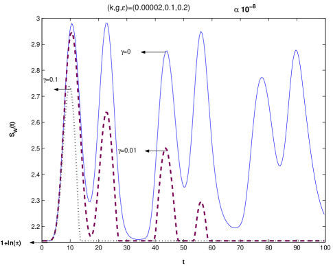
Figure 1: The time evolution of the Wehrl entropy $S_{W}(t)$  for $\alpha=10^{-8}$, ($k,g,\varepsilon$)=($0.00002,0.1,0.2$) and with different values of  $\gamma$.

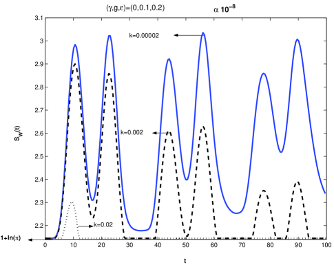
Figure 2: The time evolution of the Wehrl entropy $S_{W}(t)$  for $\alpha=10^{-8}$, ($\gamma,g,\varepsilon$)=($0,0.1,0.2$) and with different values of  $k.$

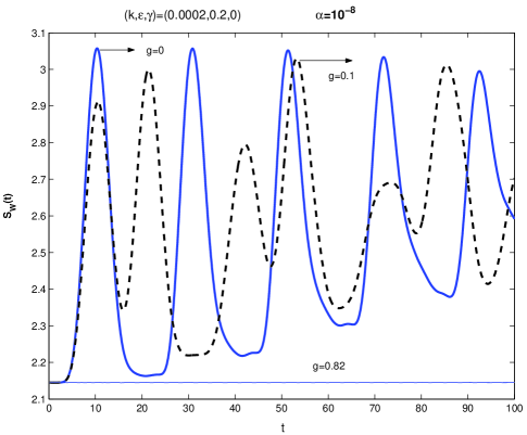
Figure 3: The time evolution of the Wehrl entropy $S_{W}(t)$  for $\alpha=10^{-8}$, ($k,\ \gamma,\varepsilon$)=(0.0002,0,0.2) and with different values of $g$.

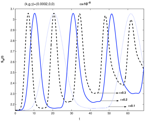
Figure 4: The time evolution of the Wehrl entropy $S_{W}(t)$  for $\alpha=10^{-8}$, ($g,\gamma,k$)=($0,0,0.0002$) and with different values of $\varepsilon$.

To explore the influence of decoherence on the dynamical behavior of the Wehrl entropy, we have plotted the time evolution of the photon Wehrl entropy $S_{W}(t)$ as a function of time $t$ for different values of the coupling constant $\gamma$ and the cavity dissipation rate $k$ in Figures.(1) and (2)
Figure.(1) shows the influences of excitonic spontaneous emission rate $\gamma$ on the Wehrl entropy (WE). By increasing $\gamma$ the (WE) decreases. Furthermore, similar effect for the cavity dissipation rate $k$ can be observed in the Fig.(2). It is worth to note that for large values of $k$ the (WE) decreases abruptly much faster than Fig.(1). The increasing of $k$ or $\gamma$ enhances the decoherence in the system and consequently causes the destruction of entanglement in the system. To have further insight, we plot in Fig.(3) and Fig.(4) the Wehrl entropy for different values of the coupling constant  $g$ and the amplitude of the driving field $\epsilon$, respectively. By increasing the coupling constant $g$ the frequency oscillation of the Wehrl entropy increases . This effect is also observed in the autocorrelation function  eleuch and in two photon excitations barzanjeh .

IV.2 Generalized concurrence

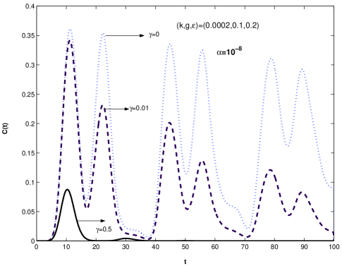
Figure 5: The time evolution of the Concurrence $C(t)$  for $\alpha=10^{-8}$, ($k,g,\varepsilon$)=(0.0002,0.1,0.2) and with different values of  $\gamma$.

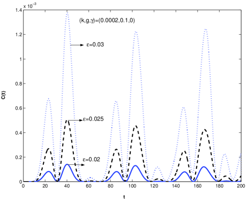
Figure 6: The time evolution of the Concurrence $C(t)$  for $\alpha=10^{-8}$, ($k,g,\gamma$)=(0.0002,0.1,0) and with different values of  $\varepsilon$.

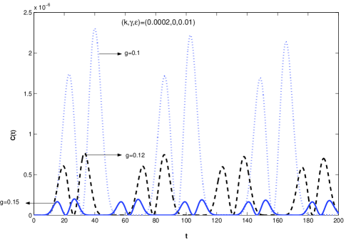
Figure 7: The time evolution of the Concurrence $C(t)$  for $\alpha=10^{-8}$, ($k,\ \gamma,\varepsilon$)=(0.0002,0,0.01) and with different values of $g$.

To study of entanglement for pure states usually the partial entropy of the density matrix is a good measure of entanglement which reads

$$\begin{array}[]{rcl}E(\psi)=-tr(\rho~{}Ln\rho)=-\sum\limits_{i}{(\lambda_{i}~{}Ln\lambda_{i})},&&\end{array}$$ (22)

where $\rho$ is the reduced density matrix, $\lambda_{i}$ is the i th eigenvalue of $\rho$. In the case of a two qubit mixed state $\rho$, the concurrence of Wootters can be used as a measure of entanglement which is given by48

$$\begin{array}[]{rcl}C(\rho)=max(0,\lambda_{1}-\lambda_{2}-\lambda_{3}-\lambda_{4}),&&\end{array}$$ (23)

in which the $\lambda_{i}$ are the square roots of eigenvalues in decreasing order of  $\sqrt{\rho}\tilde{\rho}\sqrt{\rho}$ with  $\tilde{\rho}=(\sigma_{y}\bigotimes\sigma_{y})\rho^{\ast}(\sigma_{y}\bigotimes\sigma_{y})$. Recently, some extensions have proposed for definition of concurrence in the case of an arbitrary bipartite pure state $|\psi\rangle=\sum\limits_{i=1}^{N_{1}}{\sum\limits_{j=2}^{N_{2}}{a_{ij}\left|{e_{i}\otimes e_{j}}\right\rangle}}$ as 49 ; 50

$$\begin{array}[]{rcl}C(\psi)=\sqrt{\frac{2N}{N-1}}\sqrt{\sum\limits_{i<j}^{N1}{\sum\limits_{k<l}^{N2}{\left|{a_{ik}a_{jl}-a_{il}a_{jk}}\right|^{2}}}}.&&\end{array}$$ (24)

where $N=min(N_{1},N_{2})$.
Here, we deal with a pure state $|\psi\rangle\in\mathbb{C}^{4}\bigotimes\mathbb{C}^{4}$ so that, $N=N_{1}=N_{2}=4$. To study the time evolution of the concurrence in the case of three excitations we substitute the state vector (7) into the Eq.(24), thus we obtain

$$C(\psi)=\sqrt{\frac{8}{3}\Upsilon(t)}$$ (25)

where $\Upsilon(t)$ is given by

$$\left.\begin{array}[]{r}\Upsilon(t)=\left|A_{00}A_{21}-A_{01}A_{20}\right|^{2}+\left|A_{03}A_{10}\right|^{2}+\left|A_{11}A_{03}\right|^{2}\\ +\left|A_{00}A_{11}-A_{01}A_{10}\right|^{2}+\left|A_{03}A_{12}\right|^{2}+\left|A_{02}A_{20}\right|^{2}\\ +\left|A_{01}A_{12}-A_{11}A_{02}\right|^{2}+\left|A_{20}A_{03}\right|^{2}+\left|A_{02}A_{21}\right|^{2}\\ +\left|A_{00}A_{12}-A_{12}A_{10}\right|^{2}+\left|A_{03}A_{21}\right|^{2}+\left|A_{01}A_{30}\right|^{2}\\ +\left|A_{10}A_{21}-A_{11}A_{20}\right|^{2}+\left|A_{02}A_{30}\right|^{2}+\left|A_{03}A_{30}\right|^{2}\\ +\left|A_{12}A_{20}\right|^{2}+\left|A_{21}A_{12}\right|^{2}+\left|A_{11}A_{30}\right|^{2}\\ +\left|A_{12}A_{30}\right|^{2}+\left|A_{21}A_{30}\right|^{2}\end{array}\right.$$ (33)

We plot the time dependent concurrence vector as a function of time $t$ for three values of $\gamma$ in Fig.(5). As it seen any increasing of $\gamma$ leads to decreasing of entanglement similar to the Wehrl entropy. Furthermore, an interesting cases are observed in the Fig.(6)-(7). These figures show that the concurrence is periodic in the domain of time. Moreover, unlike the large values of $\varepsilon$, figure (6) shows that entanglement can fall abruptly to zero (the two lower curves in the figure) for small values of $\varepsilon$($\varepsilon=0.025$ and $\varepsilon=0.02$), and remains zero for a period of time before entanglement recovers. The abrupt disappearance of entanglement that persists for a period of time is referred to as sudden death of entanglement (ESD)yu1 ; yu12 ; newref1 ; newref2 and also the fast appearance of entanglement after a while is called sudden birth of entanglement(ESB)yona ; lop . The length of the time interval for the zero entanglement is dependent on the values of $\varepsilon$. The smaller values of $\varepsilon$, the longer the state will stay in the disentangled separable state. Furthermore we show that the (ESD) and (ESB) can be affected strongly by the coupling constant $g$. As it is seen from figure.(7) the (ESD) and (ESB) can be enhanced by increasing of coupling constant $g$. We point out that, in the Figures.(5)-(7) we assume the zero value of the excitonic spontaneous emission rate  $\gamma=0$, thus one important reason for the (ESD) is the interaction of system with its surrounding.

IV.3 Wehrl Phase distribution

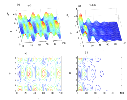
Figure 8: The time evolution of the Wehrl PD $S_{\Theta}(t)$  for $\alpha=10^{-8}$, ($k,g,\varepsilon$)=(0.0002,0,0.2) and with different values of  $\gamma$.

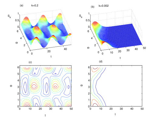
Figure 9: The time evolution of the Wehrl PD $S_{\Theta}(t)$  for $\alpha=10^{-8}$, ($\varepsilon,g,\gamma$)=(0.2,0,0) and with different values of  $k$.

The Wehrl phase distribution (Wehrl PD), defined to be the phase density of the Wehrl entropy abotalb09 ; mira3 , i.e.,

$$S_{\Theta}(t)=-\int Q_{ph}\left(\beta,\Theta,t\right)\ln Q_{ph}\left(\beta,\Theta,t\right)\left|\beta\right|d\left|\beta\right|,$$ (35)

where $\Theta=\arg\left(\beta\right)$ and $Q_{ph}\left(\beta,\Theta,t\right)$ is given in Eq.(12).

Based on Eq. (35), we present some interesting results for the effects of excitonic spontaneous emission and the dissipative rate of the cavity on the entanglement behavior in the point of view of Wehrl PD. It is observed that when $\gamma=0$ (see fig.8(a)) $S_{\Theta}(t)$ oscillates between maximum and minimum peaks which is an indication of ESB and ESD. For $\gamma\neq 0$ the situation is completely different, the excitonic spontaneous emission destroys the entanglement (see fig.8).

Now, we would like to answer the question: How $S_{\Theta}(t)$, is influenced by the cavity dissipation?  For this purpose, we take two different values of $k$ in fig.9. For small values of $k$ $S_{\Theta}(t)$ oscillates but when $k$ increases $S_{\Theta}(t)$ decreases quickly without oscillation(see figure 9(b)). This shows a one-to-one correspondence between the behavior of $S_{\Theta}(t)$ and the Wehrl entropy or concurrence which opens the door for using $S_{\Theta}(t)$ as an entanglement measure.

V Conclusion

In this paper we have studied the dynamical behavior of the quantum entanglement for a semiconductor microcavity containing a quantum well. The system is pumped with weak laser amplitude. We studied the time evolution of entanglement between the photon-exciton by the field Wehrl entropy, generalized concurrence and Wehrl phase distribution. Our results show that the new features such as entanglement sudden death and entanglement sudden birth can be reported for specific values of the cavity dissipation rate and the excitonic spontaneous emission rate.

References

- (1) A. Abeyesinghe et al., IEEE Trans. Info. Theo. 52, 3635 (2006).
- (2) C.H. Bennett, et al., Phys. Rev. Lett. 70 1895 (1993).
- (3) P. Agrawal and A. Pati, Phys. Rev. A 74, 062320 (2006).
- (4) M. B. Plenio, S. Virmani, Quant. Inf. Comp. 7, 1 (2007).
- (5) M. Zukowski, A. Zeilinger, M. A. Horne, A. K. Ekert, Phys. Rev. Lett. 71 4287 (1993).
- (6) Thorwart and co-workers, Chem. Phys. Lett. 478 234 (2009).
- (7) Xian-Min Jin, et al., Nature Photonics 4, 376 (2010).
- (8) M. Yönaç¸ T. Yu and J. H. Eberly, J. Phys. B39, 621 (2006).
- (9) L. Diósi, L. N. P., 622, 157 (2003).
- (10) S. Chan, M. D. Reid and Z. Ficek, J. Phys. B. 42, 0953 (2009).
- (11) K. Barrada et al., International Journal of Modern Physics B 23, 2021 (2009).
- (12) K. Barrada et al., Quantum Inf Process 9, 13 (2010).
- (13) K. Barrada et al., International Journal of Modern Physics C 21, 291 (2010).
- (14) C. E. Shannon and W. Weaver 1949 ”The Mathematical Theory of Communication” (Urbana University Press, Chicago).
- (15) von Neumann J 1955 ”Mathematical Foundations of Quantum Mechanics” (Princeton University Press, Princeton, NJ).
-
(16)
A. Wehrl Rev. Mod. Phys. 50 221 (1978);
A. Wehrl Rep. Math. Phys. 30 119 (1991). - (17) S. Abdel-Khalek Phys. Scr. 80 045302 (2009).
- (18) V. Bužek, C. H. Keitel and P. L. Knight Phys. Rev. A 51 2575 (1995); Watson J B, Keitel C H, Knight P L and Burnett K Phys. Rev. A 54 729 (1996).
- (19) A. Orlowski, H. Paul and G. Kastelewicz Phys. Rev. A 52 1621 (1995).
- (20) A. Anderson and J. J. Halliwell Phys. Rev. D 48 2753 (1993).
- (21) A. Miranowicz, H. Matsueda and M. R. B. Wahiddin J. Phys. A: Math. Gen. 33 5159 (2000); A. Miranowicz, J. Bajer, M. R. B. Wahiddin and N. Imoto J. Phys. A: Math. Gen. 34 3887 (2001).
- (22) I. Jex and A.Orlowski J. Mod. Opt. 41 2301 (1994).
- (23) A-S F. Obada and S. Abdel-Khalek J. Phys. A: Math. Gen. 37 6573 (2004).
- (24) S. Abdel-Khalek Physica. A 387 779 (2008).
- (25) T. Yu and J. H. Eberly, Phys. Rev. Lett. 93;140404 (2004).
- (26) T.Yu and J. H. Eberly 2002 Phys. Rev. B 66 193306; 68 165322 (2003)
- (27) T. Yu and J. H. Eberly, Opt. Commun. 264, 393 (2006).
- (28) T. Yu and J. H. Eberly, Phys. Rev. Lett. 97, 140403 (2006).
- (29) T. Yu and J. H. Eberly, Science 323, 598 (2009).
- (30) Muhammed Yönac , Ting Yu and J H Eberly, J. Phys. B 39, 621 (2006).
- (31) C. E. López, G. Romero, F. Lastra, E. Solano, and J. C. Retamal, Phys. Rev. Lett. 101, 080503 (2008).
- (32) Shan C J, Xia Y J, Acta. Phys. Sin. 55 1585 (2006).
- (33) Man Z X, Xia Y J and An N B, J. Phys. B 41 085503(2008).
- (34) Almeida M P, de Melo F, Hor-Meyll M, Salles A, Walborn S P, Ribeiro P H S and Davidovich L, Science 316, 579 (2007).
- (35) Salles A, de Melo F, Almeida M P, Hor-Meyll M, Walborn S P, Ribeiro P H S and Davidovich L, Phys. Rev. A 78, 022322(2008).
- (36) C. Ciuti et all, Phys. Rev. B. 58, R10123 (1998).
- (37) F. Tassone and Y. Yamamoto, Phys. Rev. B. 59, 10830(1999).
- (38) H. Haug, Z. Phys. B. 24, 351(1976).
- (39) E. Hanamura, J. Phys. Soc. Japan. 37, 1545 (1974).
- (40) A. B. Naguyen, Phys. Rev. B. 48, 11732(1993).
- (41) H. Eleuch, Applied Mathematics and Information Sciences. 3, 185 (2009).
- (42) A. Baas et al., Phys. Rev. A. 69, 3809(2004).
- (43) E. Giacobino et al., Comptes Rendus Physique. 3, 41(2002).
- (44) C. Ciuti, P. Schwendimann, B. Deveaud, and A. Quattropani, Phys. Rev. B. 62, R4825 (2000).
- (45) H. Eleuch, J. Phys. B. 41, 055502(2008).
- (46) G. Messin et al., J. Phys. 11, 6069(1999).
- (47) H. Eleuch et al., J. Opt. B. 1, 1(1999).
- (48) H. Eleuch and R. Bennaceur, J. Opt. A5, 528 (2003)
- (49) W. H. Louisell, Quantum Statistical Propperites Of Radiation (New York: Wiley) (1973).
- (50) H. Eleuch, Euro. Phys. J. D. 49, 391(2008).
- (51) H. Eleuch, Euro. Phys. J. D. 48, 139(2008).
- (52) H. Eleuch and N. Rachid, Eur. Phys. J. D. 57, 259 (2010).
- (53) H. Jabri et al., Physica scripta 73, 397 (2006).
- (54) H. J. Carmichael, Statistical Methods in Quantum Optics2 (Berlin: Springer) (2007).
- (55) H. J. Carmichael, R. J. Brecha, and P. R. Rice, Opt. Commun. 82, 73(1991).
- (56) R. J. Brecha, P. R. Rice, and M. Xiao, Phys. Rev. A. 59, 2392(1991).
- (57) H. Jabri et al. Laser Phys. Lett. 2, 253(2005).
- (58) C. H. Bennett, D. P. DiVincenzo, J. A. Smolin, and W. K. Wootters, Phys. Rev. A. 54, 3824(1996).
- (59) H. Eleuch, J. Phys. B. 41, 055502(2008).
- (60) Sh. Barzanjeh and H. Eleuch, Physica. E. 42, 2091(2010).
- (61) W. K. Wootters, Phys. Rev. Lett. 80, 3824(1998).
- (62) S. Albeverio, and S. M. Fei, J. Opt. B: Quantum Semiclass. Opt. 3, 1(2001).
- (63) S. J. Akhtarshenas, J. Phys. A: Math. Gen. 38, 6777 (2005).
- (64) L-H. Sun, G-X Li and Z. Ficek, Appl. Math. Inf. Sci. 4 315 (2010) ; Z. Ficek, Appl. Math. Inf. Sci. 3 375 (2009).
- (65) J-S Zhang, Ai-Xi Chen, M. Abdel-Aty J. Phys. B: At. Mol. Opt. Phys. 43 025501 (2010) ; M. Abdel-Aty Laser phys. 19 511 (2009)