Incoherent scatterer in a Luttinger liquid: a new paradigmatic limit

Abstract

We address the problem of a Luttinger liquid with a scatterer that allows for both coherent and incoherent scattering channels. The asymptotic behavior at zero temperature is governed by a new stable fixed point: a Goldstone mode dominates the low energy dynamics, leading to a universal behavior. This limit is marked by equal probabilities for forward and backward scattering. Notwithstanding this non-trivial scattering pattern, we find that the shot noise as well as zero cross-current correlations vanish. We thus present a paradigmatic picture of an impurity in the Luttinger model, alternative to the Kane-Fisher picture.

The electron-electron interaction manifests itself in a particularly pronounced way in 1D systems, inducing a strongly correlated electronic state depicted by the Luttinger liquid (LL) models Luttinger . Experimental manifestations of the latter are ubiquitous and include carbon nano-tubes, semiconductor etched edges, polymer nanowires, quantum Hall edges and more. Early on in the history of this field it has been realized that the presence of even a single weak impurity in such systems gives rise to dramatic effects single_impurity . This has been established in the seminal work of Kane and Fisher KF who studied the scaling of impurity induced backscattering in the regime of repulsive electron-electron interaction. The emerging picture has been generalized to the chiral edges of quantum Hall setups, and was extended to include observables such as shot noise. In short, the Kane-Fisher (KF) picture implies that there are two asymptotic limits of a backscattering impurity: the vanishing impurity strength (represented by an unstable fixed point): impinging particles are scattered forward (we refer to this as a $(a,1-a)$ splitter with $a=0$ being the backscattering probability.) The other limit corresponds to the infinite strength impurity (a stable fixed point): the impinging current is all backscattered, i.e. a $(1,0)$ scatterer.

The ’impurity’ in the KF setup represents the paradigmatic limit of an elastic quantum scatterer, perturbing a system of two fully coherent left and right moving modes. The complementary limit of fully incoherent scattering was studied by Furusaki and Matveev Matveev in a model where charge transmission was solely due to inelastic excitation (’inelastic co-tunneling’) of a connecting quantum dot. In general, however, scattering regions in quasi one-dimensional conductors may comprise both coherent and incoherent channels of transmission and reflection, which leads to setups intermediate between the two limits above. For example, the action of gates on a quantum Hall bar may effectively form compressible ‘quantum dots’, which arguably support both, elastic scattering channels, and inelastic scattering via bulk gapless excitations (cf. Fig. 1), for an experimental demonstration see Roddaro+05 . Similarly, the counter-propagation of edge modes along graphene pn-junctions snake is governed by a combination of single particle scattering and mode interaction, which should again lead to admixtures of coherent/incoherent transmission.

In this Letter, we explore the physics of a scattering region in which all symmetry-allowed scattering channels between two incoming and two outgoing chiral quantum wires are present (cf. Fig. 1.) We will show that the low energy properties of this system differ profoundly from those of the KF paradigm, and related models Nayak-multiple-lead ; Egger ; Chamon ; Barnabe-Theriault ; Das-Rao1 ; Giuliano ; Bellazzini ; Das-Rao2 ; Das-Rao3 ; Oreg . Specifically, we find that its conduction properties are governed by a stable fixed point at which the system becomes a $({1\over 2},{1\over 2})$ scatterer. This limit is robust and insensitive to details concerning the leads/scatterer coupling. In the vicinity of the fixed point, the model shows a number of remarkable features. Most important, and notwithstanding the fact that we deal with a non-trivial scatterer (with a finite reflection amplitude), there is neither diagonal nor cross-current shot noise. These features reflect the presence of a single gapless mode in the problem, which is protected by symmetry and evolves in a linear, and hence noiseless manner.

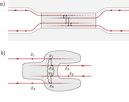
Figure 1: (Color online) Quantum wire comprising two incoming ($l=1,2$) and two outgoing $(l=3,4$) chiral modes connecting to an extended scattering region. Wiggly lines denote coherent scattering channels, dark shading represents a region of capacitive charging (the quantum dot). (a) Cartoon of possible real space structure in FQHE geometry subject to gating, (b) alternative view adjusted to our modeling with its tunneling ’hot-spots’ $x_{i}$ and lead observation points $\tilde{x}_{l}$.

Our model is depicted in Fig. 1a. Two (chiral) incoming and two (chiral) outgoing channels are coupled to a scattering ’quantum dot’ (QD). Depending on the context, the incoming chiral channels may represent edge modes of a fractional quantum hall bar, or the effectively left and right moving modes FisherGlazman of an interacting quantum wire. Charge excitations arriving in the QD may create outgoing charge, either by direct quasiparticle scattering, or indirectly, via the creation of charge excitations on the dot (cf. Fig. 1b.) Our quantitative modeling, inspired by earlier work by Furusaki and Matveev, is described by the Keldysh action $S=S^{(0)}+S_{C}+S_{\mathrm{tun}}+S_{V}.$ Here $S^{(0)}=\sum_{l=1}^{4}S_{l}^{(0)}$ represents the quadratic bosonic action of the chiral wires,

$$S_{l}^{(0)}[\phi]={\hbar\over 2}\int{dq\over 2\pi}\int{d\omega\over 2\pi}\,\phi^{T}_{i,q,\omega}\,\hat{G}^{-1}_{q,\omega}\,\phi_{i,-q,-\omega},$$ (1)

where the fields $\phi\equiv(\phi_{c},\phi_{q})^{T}$ comprises the classical and quantum Keldysh components of the boson modes describing excitations of the quantum wires. The (inverse) Keldysh Green function $\hat{G}^{-1}\equiv\left(\begin{smallmatrix}0&(G^{-})^{-1}\cr(G^{+})^{-1}&(G^{-1})^{K}\end{smallmatrix}\right)$ contains the advanced/retarded component $(G^{\pm})_{q,\omega}^{-1}={1\over 2\pi\nu}(-vq^{2}-q(\omega\pm i\delta))$, where $\nu$ may be the filling fraction of an FQHE-bar, or a measure of the interaction strength of a quantum wire FisherGlazman , and the Keldysh component $(G^{-1})^{K}={i\delta\over\pi\nu}qF(q)$, where $F$ is related to the single particle distribution function; at equilibrium $F(q)=\coth(\hbar vq/2T)$, and $\delta(\omega-vq)F(q)\equiv F_{\omega}\delta(\omega-vq)$, where $F_{\omega}=\coth(\hbar\omega/2T)$. Hereafter we put $\hbar=1$, and set the electron charge $e_{0}=1$.

The charging action

$$S_{C}[\phi]\equiv{1\over 2C}\int dt\,\left(Q\sigma_{1}Q\right),$$ (2)

accounts for the finiteness of the electrostatic capacitance, $C$, of the quantum dot. Here, $\sigma_{1}$ is a Pauli matrix, acting in Keldysh space, and

$$Q\equiv\sum_{l}Q_{l}={1\over 2\pi}(\phi_{3,d}+\phi_{4,d}-\phi_{1,d}-\phi_{2,d}),$$ (3)

is the total charge on the dot. It is given by the sum of the four charges $Q_{l}$ carried by the modes within the dot region, where $Q_{1/2}=-{1\over 2\pi}\phi_{1/2,d},Q_{3/4}={1\over 2\pi}\phi_{3/4,d}$, $\phi_{ld}\equiv\phi_{l}(x_{l})$ is the field of the $l^{th}$ wire evaluated next to the lead-dot contact point (cf. Fig. 1b), and a constant defining the charge neutrality point has been ignored.

The coherent scattering of quasi-particles from incoming leads, $i=1,2$ to outgoing leads $o=3,4$ is described by the non-linear action

$$S_{\mathrm{tun}}[\phi]=\sum_{i=1,2;o=3,4}\gamma_{ij}\sum_{s=\pm}\int dt\,\times$$ (4)

$$\times\cos\left(\phi_{i,d,c}(t)+s{\phi_{i,d,q}(t)\over 2}-\phi_{o,d,c}(t)+s{\phi_{o,d,q}(t)\over 2}\right),$$

where $\gamma_{ij}$ is the amplitude for elastic scattering from lead $i$ to $j$ at ’scattering hotspots’ within the dotPnote . Finally, we assume that one of the incoming wires, $i=1$, is subject to a bias voltage. We model the latter as a voltage kink of time-modulated hight $V(t)$ and extension from $-L\to-\infty$ to $-a<0$. The corresponding action reads $S_{V}[\phi_{1}]=\int dt\,(\phi_{1,q}(-a,t)-\phi_{1,q}(-L,t))V(t)$.

Our next step is to integrate over the bosonic fields, barring the QD-lead contact points, $x_{l}$. We obtain a zero-dimensional action

$$S=S_{\mathrm{dis}}+S_{C}+S_{\mathrm{tun}}+\tilde{S}_{V},$$ (5)

where the dissipative action reads

$$S_{\mathrm{dis}}[\phi]={1\over 2\pi\nu}\sum_{l}\int{d\omega\over 2\pi}{i\omega\over 2\pi}\phi_{l,d,-\omega}^{T}\left(\begin{smallmatrix}&-1\cr 1&2F_{\omega}\end{smallmatrix}\right)\phi_{l,d,\omega}\ ,$$

and $\tilde{S}_{V}[\phi_{1}]=-2\int{d\omega\over 2\pi}\phi_{1,q,-\omega}V_{\omega}$. In order to isolate the gapless modes of the problem, we transform to the basis

$$\Phi_{1} =(\phi_{1,d}-\phi_{2,d}+\phi_{3,d}-\phi_{4,d})/2,$$ (6)

$$\Phi_{2} =(\phi_{1,d}-\phi_{2,d}-\phi_{3,d}+\phi_{4,d})/2,$$ (7)

$$\Phi_{3} =(\phi_{1,d}+\phi_{2,d}-\phi_{3,d}-\phi_{4,d})/2,$$ (8)

$$\Phi_{4} =(\phi_{1,d}+\phi_{2,d}+\phi_{3,d}+\phi_{4,d})/2,$$ (9)

where $\Phi_{1},\Phi_{2}$ and $\Phi_{3}$ appear as arguments of $S_{\mathrm{tun}}$ and of $S_{c}$. Under renormalization they become massive, hence irrelevant to the low energy dynamics. The latter is dominated by the mode $\Phi\equiv\Phi_{4}$, whose action is

$$S[\Phi]=2\int{d\omega\over 2\pi}\,\left[{i\omega\over\pi\nu}\Phi_{-\omega}^{T}\left(\begin{smallmatrix}0&-1\cr 1&2F_{\omega}\end{smallmatrix}\right)\Phi_{\omega}-\Phi_{q,-\omega}V_{\omega}\right].$$ (10)

The independency of this action on scattering parameters and dot capacitance hints at universal behavior emerging in the low frequency scaling limit. The origin of this universality is that $\Phi$ is a soft mode related to overall charge conservation in the system; unlike with $\Phi_{1,2,3}$ this mode is protected against scattering.

To define physical observables (e.g. current, response functions) probing the universal physics of the system, we must refer to field fluctuations at representative points (‘observation points’), $\tilde{x}_{l}$, $l=1,\dots,4$, on the leads (cf. Fig. 1.) Expressed in terms of the native fields, the current at these points is given by $j_{l,c,\omega}={1\over 2\pi}\partial_{x}\phi_{l,c,\omega}(\tilde{x}_{l})$. We aim to compute current correlation functions in the low frequency limit where only the universal mode $\Phi$ prevails. To this end, we employ the identity

$$I_{l,\omega} \equiv\langle j_{l,c,\omega}\rangle=\langle\Xi_{l,\omega}\rangle_{\Phi},$$ (11)

$$X_{ll^{\prime},\omega} \equiv\langle j_{l,c,\omega}j_{l^{\prime},c,-\omega}\rangle=\langle\Xi_{l,\omega}\Xi_{l^{\prime},-\omega}\rangle_{\Phi},\qquad l\not=l^{\prime},$$

$$\quad\Xi_{l,\omega}\equiv{1\over 2\pi}(\partial_{\tilde{x}_{l}}G(\tilde{x}_{l}-x_{l})(G(0))^{-1}\Phi)_{c,\omega}+{\nu\over 2\pi}V_{\omega}\delta_{l,1},$$

where we note that the coordinate representation of the lead Green functions depends only on coordinate differences and the angular brackets on the left and right side denote functional averaging over the full action and the action of the zero mode, respectivelyCnote . In the low frequency limit $(x_{1}-x_{1,d})\omega\to 0$, the Green functions do not depend on positions explicitly anymore but still describe the causal relation between different spatial points. The quadraticity of the Goldstone mode action allows us to compute the correlation functions (11) explicitly.

Conductance —. Evaluating the first of the correlation functions (11) for the biased incoming lead, $l=i=1$, we find $I_{1,\omega}={\nu\over 2\pi}V_{\omega}$, while, evidently, there is no incoming current in the other lead, $I_{2,\omega}=0$. As for the outgoing currents ($o=3,4$) we obtain a linear current voltage characteristic

$$I_{o,\omega}={\nu\over 2\pi}{V_{\omega}\over 2},$$ (12)

which implies current conservation and conductance coefficients

$${\cal G}_{io}={1\over 2}{\nu\over 2\pi},$$ (13)

between incoming and outgoing leads. In other words: the gapless mode $\Phi$ describes an $({1\over 2},{1\over 2})$-beam splitter. For finite temperatures/AC-frequencies, the conductance coefficients will show scale dependent corrections to the $({1\over 2},{1\over 2})$ limit, which non-universally depend on the bare values of coupling constantsSnote .

Equilibrium noise —. We next analyze noise and cross-current correlations in the system. In thermal equilibrium, i.e. no external voltage bias, $V=0$, we obtain the intra-wire noise by employing a generalization of the identity Eq.(11) to the case of two fields in the same wire Cnote and find

$$X_{ll,\omega}={\nu\over 2\pi}\omega F_{\omega}$$ (14)

for all $l=1,\dots,4$. Notice that the combination $\omega F_{\omega}$ crosses over from $|\omega|$ for $|\omega|>T$ to thermal scaling $2T$ for $|\omega|<T$. We thus conclude that the low frequency intra wire noise in our system is thermal. For the cross-wire correlations we use Eq.(11) and obtain the following results:

outgoing/outgoing $$\;X_{oo^{\prime},\omega}=0,$$ (15)

incoming/outgoing $$\;X_{io,\omega}={\nu\over 4\pi}\,\omega F_{\omega},$$ (16)

incoming/incoming $$\;X_{ii^{\prime},\omega}=0.$$ (17)

The intriguing observation here is the absence of correlations between different outgoing and incoming wires. For the incoming wires, this result appears intuitive: there is no causal connection between different wires, i.e. two different incoming wires simply do not know about each other. For the outgoing leads this is less evident. However, outgoing and incoming wires can be mapped onto each other by a time reversal operation, and this suggests that their (equal time) fluctuation behavior should be identical. We note that Eqs. (13), (14), and (15) satisfy the fluctuation-dissipation theorem. Finally, current conservation, $\sum_{i=1}^{2}j_{i,c,\omega}=\sum_{o=3}^{4}j_{o,c,\omega}$, requires that for any fixed index $i_{0}=1,2$, $\sum_{i=1}^{2}X_{i_{0}i}=\sum_{o=3}^{4}X_{i_{0}0}$, a sum-rule manifestly fulfilled by Eqs. (14) and (15).

Nonquilibrium noise —. Here we are back to the situation where one of the incoming wires, $i$, is voltage biased. We first discuss current correlations between the incoming wires. There are no correlations between the biased incoming mode and the grounded mode. Turning to correlations between the incoming biased and the outgoing wires, we find

$$X_{io,\omega} = {\nu\over 4\pi}\left({\omega F_{\omega}}+{\nu\over 2\pi}|V_{\omega}|^{2}\right),$$ (18)

which fixes the incoming auto-correlation

$$X_{ii,\omega}={\nu\over 2\pi}\left(\omega F_{\omega}+{\nu\over 2\pi}|V_{\omega}|^{2}\ \delta_{i,1}\right).$$ (19)

by current conservation. Eqs. (18,19), and our above results on the average current determine the cumulants, $S_{ll^{\prime}}\equiv X_{ll^{\prime}}-\langle I_{l}\rangle\langle I_{l^{\prime}}\rangle$ as

$$S_{io,\omega}={\nu\over 2\pi}{\omega F_{\omega}\over 2},\qquad S_{ii,\omega}={\nu\over 2\pi}{\omega F_{\omega}}.$$ (20)

Remarkably, this result coincides with Eq.(15). In other words: the noise is purely thermal, there is no shot noise in the incoming wire, and no $V$-dependent correlations to the current in the outgoing wires foot_T .

Turn to correlations in the outgoing wires, we apply Eq. (11) once more to obtain

$$X_{oo^{\prime},\omega} = \left({\nu\over 4\pi}\right)^{2}|V_{\omega}|^{2}$$

$$X_{oo,\omega} = \left({\nu\over 4\pi}\right)^{2}|V_{\omega}|^{2}+{\nu\over 2\pi}{\omega F_{\omega}}$$ (21)

for the inter- ($o\not=o^{\prime}$) and intra- ($o=o^{\prime}$) wire correlations, resp. As in the bias-neutral case above, these results respect current conservation. Subtraction of the average currents yields the noise cumulants ($o\not=o^{\prime}$)

$$S_{oo,\omega}={\nu\over 2\pi}{\omega F_{\omega}},\qquad S_{oo^{\prime},\omega}=0,$$ (22)

i.e. in spite of the splitting of the incoming current into two outgoing channels, the corresponding noise remains thermal, and there are no inter-wire correlations.

The picture above is based on a rather robust physical mechanism: of the four modes supported by the two incoming and two outgoing wires, three get frozen by a combination of quasiparticle scattering and interaction, or, more technically, the simultaneous presence of more than two independent and relevant contributions to the effective action of the dot. While the freezing of all relative fluctuations, $\Phi_{1,2,3}$, in the system is responsible for the $({1\over 2},{1\over 2})$ division of conductance coefficients, one collective mode, $\Phi$, is protected by current conservation. (In fact, $\Phi$ may be interpreted as the Goldstone mode corresponding to the gauge fixing of the boson fields.) The quadratic nature of the action $S[\Phi]$, Eq. (10), signals the absence of ’charge quantization’ effects in the low frequency dynamics of the system. In particular, it implies the absence of noise, beyond the ’thermal noise’ carried by the distribution $F$. However, this result requires careful consideration: at finite $V$, the quantum scatterer, is kept in a non-equilibrium steady state, implying that $F$ might be characterized by an effective, voltage dependent, temperature, $T_{\mathrm{eff}}(V)$. The absence of shot noise notwithstanding, this $T_{\mathrm{eff}}(V)$ may give rise to voltage dependent current fluctuations, similar to those caused by shot noise. However, genuine shot noise would also generate non-vanishing cross-current correlations in the outgoing channels anti . The vanishing of these, therefore, has smoking gun status in signaling the absence of shot noise in our system.

The generality of this picture suggests various candidates to confirm its predictions in experiment. One example would be a quantum Hall strip (in the fractional regime) a finite section of which has been tuned to be in a compressible filling factor by gates. Another intriguing possibility is that the value of $1/2$ observed for the conductance of inhomogeneous graphene p-n junctions snake is due to the survival of only a single transmitting mode, along the lines of the mechanism discussed here.

We acknowledge useful discussions with P. Brouwer, B. Halperin, and M. Heiblum. This work was supported by BMBF, GIF, ISF, Minerva Foundation, SFB/TR 12 of the Deutsche Forschungsgemeinschaft, and EU GEOMDISS.

References

- (1) A.O. Gogolin, A.A. Nersesyan, and A.M. Tsvelik, Boson- ization in Strongly Correlated Systems, (University Press, Cambridge 1998); M. Stone, Bosonization (World Scientific, 1994); T. Giamarchi, Quantum Physics in One Dimension (Claverdon Press Oxford, 2004); D.L. Maslov, in Nanophysics: Coherence and Transport, edited by H. Bouchiat, Y. Gefen, G. Montambaux, and J. Dalibard (Elsevier, 2005), p.1.; J. von Delft and H. Schoeller, Annalen Phys. 7, 225 (1998).
- (2) A. Luther and I. Peschel, Phys. Rev. B 9, 2911 (1974); D. C. Mattis, J. Math. Phys. 15, 609 (1974).
- (3) C.L. Kane and M.P.A. Fisher, Phys. Rev. B. 46,15233 (1992).
- (4) A. Furusaki and K. A. Matveev, Phys. Rev. Lett. 75, 709 (1995); Phys. Rev. B 52, 16676 (1995).
- (5) S. Roddaro, V. Pellegrini, F. Beltram, L.N. Pfeiffer, and K.W. West, Phys. Rev. Lett. 95, 156804 (2005).
- (6) S. Nakaharai, J. R. Williams, and C. M. Marcus, preprint arXiv:1010.1919 (2010).
- (7) C. Nayak, M. P. A. Fisher, A. W. W. Ludwig, and H. H. Lin, Phys. Rev. B 59, 15694 (1999); see also I. Affleck and J. Sagi, Nucl. Phys. B417, (1994) 374.
- (8) S. Chen, B. Trauzettel, and R. Egger, Phys. Rev. Lett. 89, 226404 (2002); R. Egger et al., New Journal of Physics 5, 117 (2003).
- (9) C. Chamon, M. Oshikawa, and I. Affleck, Phys. Rev. Lett. 91, 206403 (2003); M. Oshikawa, C. Chamon, and I. Affleck, J. Stat. Mech. J.Stat.Mech. 0602 (2006) P02008.
- (10) X. Barnabe-Theriault et al., Phys. Rev. B 71, 205327 (2005); Phys. Rev. Lett. 94, 136405 (2005).
- (11) S. Das, S. Rao, and D. Sen, Phys. Rev. B 74, 045322 (2006).
- (12) D. Giuliano and P. Sodano, Nucl. Phys. B 811, 395 (2009); New Journal of Physics 10, 093023 (2008).
- (13) B. Bellazzini et al., arXiv:0801.2852; B. Bellazzini, P. Calabrese, and M. Mintchev, Phys. Rev. B 79, 085122 (2009).
- (14) S. Das and S. Rao, Phys. Rev. B 70, 155420 (2004).
- (15) A. Agarwal et al., Phys. Rev. Lett. 103, 026401 (2009).
- (16) Y. Oreg and A. M. Finkelstein, Phil. Mag. B 77, 1145 1998.
- (17) M.P.A. Fisher and L.I. Glazman, in Mesoscopic Electron Transport, ed. by L.L. Sohn, L.P. Kouwenhoven, and G. Schoen. NATO ASI Series, Vol. 345, Kluwer Academic Publishers, 1997.
- (18) The detailed position of these points does not qualitatively affect our results, whence we identify them with the points above.
- (19) To prove these identities, one has to carry out the Gaussian integration leading to (5) in the presence of the pre-exponential term on the l.h.s. As a result of a straightforward if somewhat lengthy calculation one obtains the r.h.s. The current auto-correlation function, is given by a slightly more complicated expression which we do not state explicitly, as its evaluation is fixed by current conservation.
- (20) While for high temperatures/frequencies and for weak initial scattering strength , the ensuing power laws are determined by the scaling dimensions and of and , resp., for temperature/frequencies smaller than the charging term increases the scaling dimension of the to . The analysis of the crossover regimes at intermediate to strong scattering is beyond the scope of this paper. It is worth noting that the model can be fine tuned to a partially decoupled limit or where KF scaling to a fully transmitting, , or reflecting, , configuration prevails. For all other configurations, and all scale up, thus stabilizing the flow towards the limit. Another interesting limit is zero dot interaction, . Even then a conspiracy of bulk interactions, , and coherent scattering will lead to the upflow of the amplitudes . A straightforward scaling analysis shows that the approach of the stable fixed point will be slower than in the case of finite .
- (21) This result tacitly assumes that the whole system is kept at a thermal distribution characterized by some effective temperature . Heating effects may influence this temperature.
- (22) Ya.M. Blanter and M. B uttiker, Phys. Rep. 336, 1 (2000).