Thermochemical and Photochemical Kinetics in Cooler Hydrogen Dominated Extrasolar Planets:
A Methane-Poor GJ436b?

Abstract

We introduce a thermochemical kinetics and photochemical model. We use high-temperature bidirectional reaction rates for important H, C, O and N reactions (most importantly for CH₄ to CO interconversion), allowing us to attain thermochemical equilibrium, deep in an atmosphere, purely kinetically. This allows the chemical modeling of an entire atmosphere, from deep-atmosphere thermochemical equilibrium to the photochemically dominated regime. We use our model to explore the atmospheric chemistry of cooler ($T_{eff}<10^{3}$ K) extrasolar giant planets. In particular, we choose to model the nearby hot Neptune GJ436b, the only planet in this temperature regime for which spectroscopic measurements and estimates of chemical abundances now exist. Recent Spitzer measurements with retrieval have shown that methane is driven strongly out of equilibrium and is deeply depleted on the dayside of GJ 436b, whereas quenched carbon monoxide is abundant. This is surprising because GJ 436b is cooler than many of the heavily irradiated hot Jovians and thermally favorable for CH₄, and thus requires an efficient mechanism for destroying it. We include realistic estimates of ultraviolet flux from the parent dM star GJ 436, to bound the direct photolysis and photosensitized depletion of CH₄. While our models indicate fairly rich disequilibrium conditions are likely in cooler exoplanets over a range of planetary metallicities, we are unable to generate the conditions for substantial CH₄ destruction. One possibility is an anomalous source of abundant H atoms between 0.01-1 bars (which attack CH₄), but we cannot as yet identify an efficient means to produce these hot atoms.

1. Introduction

Currently, transiting extrasolar planets offer virtually exclusive opportunities for observing physical and chemical states of exoplanetary atmospheres. Over the past four years, retrievals of atmospheric molecules from multicolor transit photometry (i.e. transit spectra) have compelled the development of progressively more sophisticated atmopheric models to interpret the observations and understand underlying chemical and dynamical processes. In particular, atmospheric-chemistry modeling is evolving from strictly thermo-equilibrium models with stationary chemical species, to coupled models (Zahnle et al. 2009a,b; Line et al. 2010; Moses et al 2011) incorporating thermo-kinetics, vertical transport, and photochemistry. Thus far, such efforts have been devoted to hot-Jupiter planets, especially HD 209458b and HD 189733b, due to their favorable transit depths and eclipse brightnesses and, therefore, far greater availability of observational data. However, with the recent retrieval of molecular abundances in the atmosphere of GJ 436b (Stevenson et al. 2010; Madhusudhan & Seager 2011), exoplanetary science is venturing into a new territory: hot-Neptune atmospheric chemistry. GJ 436b is bound to serve as a prototypical planet anchoring the theoretical framework for understanding the hot-Neptune class of exoplanets, much as how HD 209458b and HD 189733b have for hot Jupiters. It is also the first planet with observable thermal emission that transits an M star. M stars are of particular interest since they constitute the majority of stars in the solar neighborhood, and they have close-in habitable zones, which enhances radial-velocity detectability and transit observability; therefore, M stars present the best opportunities to discover and characterize rocky, potentially habitable exoplanets in the near future. GJ 436b and GJ 1214b provide the only present test cases for atmospheric chemistry of planets orbiting M dwarfs. Therefore, an era of intensive investigations of this planet is commencing. This paper presents our application of a state-of-the-art model seamlessly integrating thermo-kinetics, vertical transport, and photochemistry to simulate the atmospheric chemistry of GJ 436b in a similar manner to Visscher et al. (2010) and Moses et al. (2011) , along with realisitic estimates of UV fluxes for this planet.

The first transiting hot Neptune discovered (Butler et al. 2004, Gillon et al. 2007), GJ 436b, revolves around an M dwarf merely 10 pc away from Earth and has received much attention due to its interesting orbital dynamics (Ribas et al. 2008, Mardling 2008, Batygin et al. 2009), interior properties (Nettelmann et al. 2010, Kramm et al. 2011), and atmospheric properties (Stevenson et al. 2010, Lewis et al. 2010, Madhusudhan & Seager 2011, Shabram et al. 2011). The slightly eccentric orbit (eccentricity = 0.16) has a mean orbital radius of 0.0287 AU (Torres et al. 2008), and the planet probably has a pseudo-synchronous rotation (Deming et al. 2007). The planet’s mass is 23 $M_{\oplus}$, and its density of 1.7 g/cm³ resembles that of the ice-giant Neptune (1.63 g/cm³). Analyses of its mass-radius relationship and transit depth indicates a layer of H/He dominated atmosphere is clearly required (Figueira et al. 2009; Nettelmann et al. 2010; Rogers & Seager 2010). The host star has an effective temperature of $\sim$ 3400 K and an estimated age of 3 – 9 Gyr (Torres et al. 2008). Assuming zero albedo and global thermal re-distribution, the planet’s effective temperature is 650 K. Of the confirmed transiting exoplanets (Wright et al. 2011), GJ 436b is one of the least irradiated and has one of the coolest atmospheres. Therefore, this planet represents a significant departure from hot Jupiters in terms of size, thermal environment, and UV flux.

Although GJ 436b was discovered in 2004 (Butler, by radial velocity), it was not until 2010 that a retrieval of explicit molecular abundances in its atmosphere was reported (Stevenson et al. 2010), where six channels of secondary-eclipse photometry data ranging from 3.6 to 24 $\mu$m were analyzed by generating $\sim$ 10⁶ simulated spectra using varying combinations of molecular compositions and temperature profiles to find the best fit to observations. A more recent paper (Madhusudhan & Seager 2011) provides further details and updated results of a re-analysis of the same dataset using the same general retrieval method. In short, 10⁶ combinations of ten physio-chemical free parameters, each spanning a large range of values, were used to generate synthetic dayside-emission spectra. In each of the 10⁶ scenarios, six of the ten parameters were used to define the temperature-pressure (T-P) profile, whereas the other four parameters specified vertically uniform abundances of four molecules: H₂O, CO, CH₄, and CO₂. Additionally, the 1-D atmospheric model restricted the ratio of emergent flux output to incident stellar flux input on the day side to within the range between zero and unity. Given six data points and ten free paramters, the retrieval problem was mathematically underdetermined. Nonetheless, sampling a million points in parameter-phase space allowed the authors to examine the joint probability contours, as defined by the goodness-of-fit (chi-square) function, projected on multiple-parameter spaces. Furthermore, by placing physical-plausibility constraints (in consideration of believable departures from thermo-equilibrium chemistry) on the molecular abundances, the authors were able to confine the physical space to a fairly narrow, “best-fit,” range for chi-square $\leq$ 3. Depending on the wavelength, the photospheric altitude varies from 9 bar to 0.2 bar levels. The main conclusions are as follows: 1) temperature inversion is ruled out (i.e. no stratosphere); 2) 6 ppm (parts per million) is the absolute upper limit for CH₄ abundance; 3) 300 ppm is the absolute upper limit for H₂O abundance; 4) CO₂ and CO abundances are anti-correlated; 5) taking physical-plausibility into consideration, the best-fit spectrum represents $X_{\rm H_{2}O}$ = 100 ppm, $X_{\rm CH_{4}}$ = 1 ppm, $X_{\rm CO}$ = 7000 ppm, and $X_{\rm CO_{2}}$ = 6 ppm, where $X_{\rm i}$ is the number density of molecule $i$ divided by that of H₂. Also, note that even in the best-fit scenario, $X_{CO_{2}}$ can range anywhere from 1 – 100 ppm. The Stevenson et al. (2010) and the Madhusudhan & Seager (2011) efforts are the most comprehensive studies of atmospheric composition on GJ 436b thus far.

From a theoretical point of view, the preceding abundance limits and values pose a very interesting challenge due to their drastic departures from thermo-equilibrium predictions, which indicate the following rough-order-of-magnitude values: $X_{\rm H_{2}O}$ = 1000 (3$\times$10⁴) ppm, $X_{\rm CH_{4}}$ = 1000 (10⁴) ppm, $X_{\rm CO}$ = 60 (10⁴) ppm, and $X_{\rm CO_{2}}$ = 0.1 (1000) ppm for 1x (50x) solar metallicities at $\sim 1$bar. In either metallicity scenario, water and methane remain abundant ($\geq$ 1000 ppm), whereas the retrieval shows water being relatively depleted and methane being drastically depleted. Moreover, the thermo-equilibrium abundances of carbon monoxide and carbon dioxide are positively correlated (either both low in the 1$\times$ case or both high in the 50$\times$ case), in contrast with the retrieval’s anti-correlation. In particular, the retrieved partioning of carbon overwhelmingly in oxidized species amidst a hydrogen-dominated (reducing), temperate atmosphere is very surprising. For instance, at 1-bar pressure and solar metallicity, CH₄ is the thermodynamically dominant carbon-bearing molecule for temperatures less than 1100 K (Lodders & Fegley 2002). The common practices of simply adjusting metallicity and/or the C/O ratio cannot simultaneously reconcile these discrepancies. Therefore, one must investigate disequilibrium mechanisms.

Madhusudhan & Seager (2011) posited that high metallicity combined with vertical mixing can explain the disequilibrium abundance of carbon oxides. Basically, enhanced metallicity ($\sim$ 10$\times$ solar) can provide the requisite abundance of CO₂. Since equilibrium CO abundance drops sharply with respect to temperature (Lodders & Fegley 2002) the retrieved uniformly high abundance of CO requires eddy mixing to populate upper, cooler, atmospheric layers. However, vertical eddy mixing alone cannot explain the large depletion of CH₄ due to its innately high thermochemical abundance in the deep atmosphere. Therefore, Madhusudhan & Seager (2011) invoked photochemistry as the potential culprit, based on Zahnle et al.’s (2009a,b) studies of photochemistry on hot Jupiters. In such a scheme, photosensitized sulfur chemistry produces atomic H, which then destroys CH₄ to form higher hydrocarbons. However, the Zahnle et al. (2009a,b) model uses solar-type stellar irradiance and an isothermal atmsophere (i.e. constant temperature versus altitude). As such, neither the photochemical driver nor the thermal environment is tailored for our planet in question. More severely, Moses et al. (2011) pointed out that a typo in a key rate coefficient in the Zahnle et al. (2009a,b) model caused the apparent conversion of methane into higher hydrocarbons at pressures larger than 1 mbar. Generally speaking, at pressures larger than 1 mbar in a hydrogen-abundant atmosphere, hydrogenation of unsaturated hydrocarbons and reaction intermediates efficiently recycle species back to methane, preventing its large- scale destruction. Moses et al. (2011) also discussed the inadequacies of isothermal atmospheric models due to their suppression of transport-induced quenching. Hence, the observed CH₄ depletion still awaits adequate explanation. The low abundance of H₂O also has not been addressed.

In addition to secondary eclipse observations, primary transit observations of GJ 436b exist as well (Pont et al. 2009, Ballard et al. 2010, Beaulieu et al. 2011, Knutson et al 2011), and various groups have analyzed them to retrieve molecular abundances in the planet’s terminator regions (Beaulieu et al 2011, Knutson et al 2011). In contrast to the secondary-eclipse retrieval, Beaulieu et al. (2011) were able to fit a compendium of their and Ballard et al.’s tansit observations between 0.5 and 9 $\mu$m with 500 ppm CH₄ in a H₂ atmosphere, and finding no clear evidence for CO or CO₂. Moreover, Beaulieu et al. presented that a methane-rich atmosphere, with temperature inversion, can be consistent with the said secondary-eclipse data as well (but see Shabram et al. 2011). More recently, Knutson et al. acquired Spitzer transit photometry at 3.6, 4.5, and 8.0 $\mu$m during 11 visits. The multiple-visit data showed high transit-depth variability, which the authors attribute to potential stellar activity in the dM host. They did not find any compelling evidence for methane, and data excluding ones believed to be most affected by stellar activity appear to place an upper limit of 10 ppm for methane mixing ratio. The best-fit spectrum to this select data set assumes 1000 ppm H₂O, 1000 ppm CO, 1 ppm CH₄, with CO₂ abundance poorly constrained, roughly in agreement with Madhusudhan et al. Therefore, primary-transit data is currently inconclusive due to different interpretations by different groups.

Our primary goal is to advance the fundamental understanding of processes impacting the chemical state of GJ 436b by developing a 1-D atmospheric model that integrates all of the aforementioned equilibrium and disequilibrium processes. An important aspect of our model is the seamless integration of thermochemistry, kinetics, vertical mixing, and photochemistry in a manner that directly follows from Visscher et al. (2010), and contemporaneously with Moses et al. (2011), obviating the conventional quench-level estimation (Prinn & Barshay 1977).

The quench-level approach assumes that the deep atmosphere is in thermochemical equilibrium because high temperatures provide sufficient kinetic energy to overcome reaction barriers in either direction. However, as vertical tranport lifts a gas parcel to cooler, higher altitudes, chemistry becomes rate limited rather than thermodynamically determined. There comes a point in altitude where the kinetic conversion time scale becomes slower than the transport time scale, and the rate-limiting reaction for a molecule of interest is not allowed time to reach completion. At altitudes above this point, the molecule’s concentration is frozen/quenched (therefore, the term “quench level”). In effect, the quench-level approach partitions the atmosphere into two parts: below the quench level, thermochemical equilibrium determines chemical abundances; above the quench level, molecular abundances are uniform versus altitude, with values equal to the equilibrium value at the appropriate quench level for each species. Although this approach has a long record of success (e.g., Prinn & Barshay 1977; Smith 1998; Griffith & Yelle 1999; Saumon et al. 2003; 2006; 2007; Hubeny & Burrows 2007; Cooper & Showman 2006), it does have some limiting assumptions and caveats that require great judiciousness. Specifically, one needs to determine the appropriate rate-limiting, interconversion reaction for each set of coupled species of interest (e.g., interconversion between CH₄ & CO). The correct reaction choice is not always readily apparent (see e.g., Visscher et al. 2010) and the appropriate length scale for deriving the mixing time scale from the vertical eddy diffusion coefficient ($K_{zz}$) is still under some debate. Furthermore, since a basic assumption is that temperature decreases with altitude, atmospheric temperature inversions can complicate matters.

Therefore, we implemented a fully reversible kinetic model in the following manner. Every measured forward reaction rate in our list is reversed using the equilibrium constant and the principle of microscopic reversibility. Given enough pathways, both forward and backwards, a given set of chemical species will reach thermochemical equilibrium, kinetically. This provides a seamless transition from the thermochemical equilibrium regime to the disequilibrium-dominated regimes. We can investigate the disequilibrium effects on atmospheric composition in a much more holistic, systematic manner, compared to heuristically identifying plausible disequilibrium processes.

In the remainder of this manuscript we describe the disequilibrium processes that may be occurring in GJ436b’s atmosphere. In $\S$2 we describe thermochemical and chemical kinetics models as well as our estimate for the stellar UV flux. In $\S$3 we show the modeling results as well as a description of the important reaction schemes governing the abundances of various species. Finally in $\S$4 we discuss the relevant implications and conclude.

2. Description of Models

We use joint thermochemistry and “1-D chemical-kinetics with photochemistry” models to study the atmosphere’s departure from thermal equilibrium. External inputs to our models are the metals fraction (denoted further on by $\zeta$), the pressure and temperature (T-P) profile, the eddy diffusion coefficient profile, and the incident stellar flux; note that we fix the T-P profile and the chemistry is decoupled from it, i.e., there is no self-consistent, radiative-convective adjustment of temperature structure when the chemistry is evolved towards steady state. We initialize the 1-D atmospheres using the NASA Chemical Equilibrium with Applications (CEA) model (Gordon & McBride 1996). Given the initial elemental abundances of H, He, C, O, N, and S in an atmospheric layer, along with the layer’s pressure and temperature, CEA uses a Gibbs free-energy minimization and mass balance routine to calculate the equilibrium species abundances.

Whereas chemical equilibrium concentrations are useful for initializing the atmosphere, they do not provide the correct chemical state above pressure levels of $\simeq 10$ bars (Prinn & Barshay 1977; Griffith & Yelle 1999; Cooper & Showman 2006; Line et al. 2010; Moses et al. 2011). We simply supply the equilibirum mixing-ratios as boundary conditions in the deep atmosphere for the kinetics calculations, and thereafter evolve the chemical state over multiple timesteps until a steady state is reached.

The computations are carried out with the Caltech/JPL photochemical and kinetics model, KINETICS (a fully implicit, finite difference code), which solves the coupled continuity equations for each involved species, and includes transport via molecular and eddy diffusion (Allen et al. 1981; Yung et al. 1984; Gladstone et al. 1996; Moses et al. 2005). We use the H, C, and O chemical reaction list originally described in Liang et al.(2003; 2004) and references therein updated to high temperatures, recently augmented with a set of N reactions. We have not included the chemistry of sulfur in any great detail, because much of its kinetics is poorly constrained (see e.g., Moses et al. 1996). However we do consider a small, but well measured, set of H₂S reactions. This helps us appraise if and how the introduction of S affects the abundances of the main molecular reservoirs of H, C, N, O such as CH₄.

We use high temperature rate coefficients for reactions from Line et al. (2010). All reactions are bidirectional, and we reverse them by calculating the back-reaction rates using thermodynamic data (see Table S1). With appropriate reaction pathways and proper rates for the back-reactions, the models can converge to chemical equilibrium purely kinetically in the deep planetary atmosphere where reaction timescales are short compared to transport timescales, and photochemical reactions are unimportant. As mentioned earlier, this removes the cumbersome requirement of having to choose a lower boundary for individual species through ad hoc quench-level arguments (Prinn & Barshay 1977; Smith et al. 1998).

We solve for 51 hydrogen, carbon, oxygen and nitrogen bearing species including H, He, H₂, C, CH, ¹CH₂, ³CH₂, CH₃, CH₄, C₂, C₂H, C₂H₂, C₂H₃, C₂H₄, C₂H₅, C₂H₆, O, O(1D), O₂, OH, H₂O, CO, CO2, HCO, H₂CO, CH₂OH, CH₃O, CH₃OH, HCCO, H₂CCO, CH₃CO, CH₃CHO, C₂H₄OH, N, N₂, NH, NH₂, NH₃, N₂H, N₂H₂, N₂H₃, N₂H₄, NO, HNO, NCO, HCN, CN, CH₃NH₂, CH₂NH₂, CH₂NH, H₂CN, with a total of $\sim 700$ reactions, 55 of which are photolysis reactions. The chemical pathway for reducing CO to CH₄, described recently for Jupiter’s deep atmosphere (Visscher et al. 2010), is included in our reaction list, along with the reverse pathways for CH₄ to CO oxidation. Photolysis absorption cross sections are from Moses et al. (2005) and the thermodynamic data (i.e. the compilation of entropies and enthalpies) used to reverse the kinetic rate coefficients are from JANAF and CEA thermobuild databases; e.g., CEA uses data from Chase et al. (1998) and Gurvich et al. (1989) (see Zehe et al. 2002).

2.1. Model Parameters

We model a large pressure and altitude range, 10³ to 10^-11 bars ($\sim$5000 km or $\sim$0.2 R_p from the 1 bar level), so as to capture the three major atmospheric regimes and the transitions between them. These three dominant portions of the atmosphere are – the thermal equilibrium regime in the deep hot atmosphere, the eddy transport dominated regime at intermediate pressures, and the photochemical regime at low pressures. A total of 190 pressure levels, uniform in logarithmic space, are used between the abovementioned levels, giving a resolution of about 14 levels per decade of pressure. Altitudes above the homopause remain relatively cool in our models, and we disregard the possibility of a hot thermosphere despite the models extend up to exophere levels at 10^-11 bars; this simplification has little or no bearing on the state of the atmosphere below the homopause ($P\sim 1\mu$bar). We adopt the $\zeta=1$ T-P profile from Lewis et al. (2010) (see Figure 1), noting its similarity to the T-P profile retrieved in Madhusudhan & Seager (2011) and Stevenson et al. (2010). Whereas GJ 436 itself is slightly subsolar in abundances (Bean et al. 2006), we allow for a span of planetary metallicities, covering the cases $\zeta=0.1,1,50$, and allowing for the possibility that the planet is either enriched or depleted; we used solar abundances from the standard text of Yung & DeMore (1999). For non-solar atmospheres we tune the fractions of C, N, O, and S relative to H but not relative to each-other (e.g., C/O, N/O, S/O, are always fixed).

Figure 1.— Estimated temperature profiles for GJ 436b. The dashed profile is the disk averaged dayside profile retrieved by Stevenson et al. (2010). The solid curve is the $\zeta=1$ profile from the global circulation model of Lewis et al. (2010). We use the latter T-P profile for our chemical models.

The eddy diffusion strength (parameterized by a coeffcient, $K_{zz}$) determines the pressure level at which a species is chemically quenched. At the quench level for chemical $X$, the timescale for vertical transport ($\tau_{trans}$) equals the chemical loss timescale ($\tau_{chem,X}$). Above that level, which includes the visible portion of the atmosphere, the mixing virtually “freezes” the concentration of that species. Below the quench level, $\tau_{chem,X}\ll\tau_{trans}$, and thermochemical balance is achieved. Line et al. (2010) and Moses et al. (2011) have used piecewise estimates of the eddy diffusion profiles, $K_{zz}(P)$. The recipe has been to estimate $K_{zz}$ in the deep adiabatic troposphere ($\sim 10^{3}$ bars) using mixing length theories (e.g., Flasar & Gierasch 1977) and stitch this to global circulation model (GCM) derived profiles obtained by multiplying the (horizontally averaged) GCM vertical winds of Showman et al. (2009) by the local scale height. Lewis et al. (2010) apply this procedure to their GJ 436b circulation model, and estimate that $K_{zz}$ increases from $\sim 10^{8}$ at depth (100 bars) to $10^{11}$ cm² s^-1 at lower pressures (1 mbar).

Such procedures have gnawing uncertainties – for example, the appropriate eddy mixing length may only be a fraction of the scale height, or the vertical wind strengths could well be overestimated. Smith (1998) has demonstrated theoretically that using an eddy length scale equal to the scale height is inappropriate, and may lead to gross over-estimates of the length scale ($L$) and the timescale ($\tau_{trans}=L^{2}/K_{zz}$). Herein, we simplify matters by choosing a constant $K_{zz}(P)=10^{8}$ cm² s^-1 profile; this value is similar to that for the deep atmosphere in the Lewis et al. GCM. This simplification has a couple of redeeming features. First, this gives quench levels similar to those that would be derived had we used a GCM-inspired $K_{zz}$ profile. Second, whereas a low $K_{zz}$ may underestimate the mixing strength at higher altitudes, it has the effect more lethargic replenishment of methane and other photodissociated species from the lower atmosphere (it bolsters the photochemical timescale, relative to $\tau_{trans}$).

2.2. The Ultraviolet Emission from GJ 436

dM stars such as GJ 436 show very little photospheric emission in the near to far ultraviolet (UV). Nevertheless, non-radiative energetic processes can transport energy to power a hot outer atmosphere, and this energy is partially dissipated in the form of cooling, chromospheric UV emission. Because the UV emission levels depend on many factors, ab initio estimates of it are difficult. We use GALEX and ROSAT derived estimates for GJ 436 and combine these with a $T_{eff}\simeq 3400$ K continuum from the stellar photosphere. This combined emission is used to drive photochemical reactions in GJ 436b.

In the planetary atmosphere both H₂ and He are weak absorbers relative to other molecular species, but are enormously more abundant. Helium ceases to absorb longwards of $500$ Å, and H₂ longwards of $1000$ Å. Methane, a carbon reservoir and the molecule of particular interest herein, has a large absorption cross-section shortwards of 1600 Å. Whereas methane (and water) is largely shielded by H₂ and He from very shortwave radiation, it is photodissociated by radiation between 1000-1600 Å, and is therefore susceptible to possible intense H I Ly $\alpha$ ($\lambda=1216$ Å) from the M star host. Longwards of $\lambda=1600$ Å, direct photolysis of methane dwindles due to a combination of the falling cross-section and weak stellar flux. Hydrogen sulfide photodissociates at much longer wavelengths, $\lambda<2600$ Å, and if present in substantial quantities, is poorly shielded by other reservoir molecules H₂, CH₄, H₂O, etc. H₂S photolysis and the resultant hot atomic hydrogen may be influential if $\lambda\simeq 2600$ Å photons can penetrate deep into the planetary atmosphere (more in §3.3.5).

GJ 436 is detected in a GALEX survey exposure in the near UV channel with flux $f_{nuv}=21.0\pm 3.7$ $\mu$Jy (near-UV channel, $\bar{\lambda}=2267$ Å, $\Delta\lambda_{FWHM}=616$ Å). It is undetected in the GALEX far UV band, with a $3\sigma$ upper limit of $f_{fuv}\leq 24$ $\mu$Jy (far-UV channel, $\bar{\lambda}=1516$ Å, $\Delta\lambda_{FWHM}=270$ Å). These can be converted to incident UV photon fluxes at the mean orbital separation of GJ 436b. The near UV detection implies a flux of $9\times 10^{10}$ photons cm^-2 s^-1 Å^-1 $\lambda=1960-2580$ Å at the planetary substellar point. This dosage at GJ 436b is about 0.2 PELs (present-Earth-levels); mean Solar photon flux at Earth is $4.7\times 10^{11}$ photons cm^-2 s^-1 Å^-1 between 2000-2500 Å (Yung & DeMore 1999). The $3\sigma$ flux upper bound (GALEX far-UV channel) is $\leq 1.3\times 10^{11}$ photons cm^-2 s^-1 Å^-1 $\lambda=1450-1650\AA$; this is just a factor of two higher than present-Earth-levels in an equivalent passband.

H Ly $\alpha$ emission can be powerful in the upper chromospheres of cool stars. Because it is strongly absorbed in the interstellar medium, direct line strength estimates are difficult. We make an indirect determination based on empirical correlations with soft X-ray fluxes. Soft X-ray emission from GJ 436 has been observed in the Rosat All Sky Survey (Hünsch et al. 1999), with $f_{x}\simeq 5.4\times 10^{-14}$ erg cm^-2 s^-1 (0.1-2.4 keV; Rosat PSPC), implying a fractional X-ray luminosity of $L_{x}/L_{bol}\sim 8\times 10^{-6}$; this fraction is a factor $\sim 100$ lower than that observed from the most active dM stars and is consistent with GJ436b’s estimated advanced age, $6\pm 3$ Gyr. More recent XMM-Newton EPIC measurements (Sanz-Forcada et al. 2010) give a factor of 8 lower $L_{x}$, which may well be due to X-ray activity. Herein, we adopt the ROSAT flux because larger X-ray fluxes imply proportionally larger Ly $\alpha$ fluxes.

To estimate the Ly $\alpha$ output, we use an an empirical correlation of the X-ray and Ly $\alpha$ emission of stars, derived from stellar samples that include several late type stars (e.g., Landsman & Simon 1993 and Woods et al. 2004; in these papers, measurements of Ly $\alpha$ lines were made from International Ultraviolet Explorer and Hubble Space Telescope spectra, after applying a model based correction of ISM absorption). Inverting the Woods et al. (2004) empirical power law, $\log F_{x}\simeq 2.2\log F_{Ly\alpha}-7.76$, we determine a photon flux of $f_{Ly\alpha}\sim 1.5\times 10^{14}$ photons cm^-2 s^-1 at GJ 436b. The Solar H Ly $\alpha$ flux at Earth is $\simeq 10^{12}$ photons cm^-2 s^-1, a factor 100 lower. The reliability of X-ray derived Lyman $\alpha$ line flux may be assessed by comparing $F_{Ly\alpha}$ with the GJ 436b’s H $\alpha$ line flux. H $\alpha$ observed in GJ436 in absorption, with an equivalent width of 0.32 Å  (Palomar-Michigan State Nearby Star Spectroscopic Survey; Gizis, Reid & Hawley 2002), implies a line flux of $F_{H\alpha}\simeq 2\times 10^{5}$ erg cm^-2 s^-1, and a line strength ratio of H Ly $\alpha$ to H $\alpha$ of 2.2. For dM stars, where H Ly $\alpha$ is seen in emission and for which the intrinsic Ly $\alpha$ line strengths have been measured, this line strength ratio varies between 3-5, with some stars having ratios as low as 2 and others as high as 8 (Doyle et al. 1997).

3. Chemical Model Results

3.1. Thermochemical Equilibrium

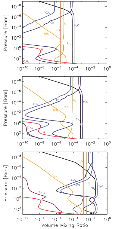
Figure 2.— Thermochemical equilibrium vertical distributions for abundant H, C, O, N, and S species assuming the temperature profile in Figure 2. Three metallicity cases are shown ($\zeta=0.1$, $1$, and $50$, from top to bottom). The thermochemical equilibrium mixing ratios are derived using the CEA Gibbs free energy minimization code for each atmospheric T-P level.

Equilibrium vertical mixing ratios for the three metallicity cases are shown in Figure 2: these are sub-solar $\zeta=0.1$, solar $\zeta=1$ and super-solar $\zeta=50$ heavy elemental abundances. Because GJ 436b is significantly cooler than HD 189733b and HD 209458b, CH₄ is the thermochemically favored carbon carrier; higher effective temperatures drive equilibrium towards CO in the two hot Jupiters. The thermochemical abundances of CH₄, CO and H₂O along the T-P profile are readily understood through the net reaction

$${\rm CO+3H_{2}}\rightleftharpoons{\rm CH_{4}+H_{2}O}$$ (1)

along with the Law of Mass Action:

$$\frac{X_{CH_{4}}X_{H_{2}O}}{X_{CO}X^{3}_{H_{2}}}\frac{1}{P^{2}}=K_{eq}(T)$$ (2)

derived by minimizing the Gibbs free energy of net reaction in (1), with the mixing ratio $X_{i}$ of species $i$, with ambient pressure $P$, and a temperature dependent equilibrium constant $K_{eq}(T)$; the $T$ dependence is governed by the van ’t Hoff equation ($\Delta G=-RT\log K_{eq}$, with $\Delta G$ as the standard Gibbs free energy change). At a given pressure $P$, $K_{eq}(T)$ behaves in a manner that rising $T$ drives the equilibrium towards CO. At a fixed $T$, increasing/decreasing pressures favor higher CH₄/CO concentrations. These relationships are exemplified in the $\zeta=1$ equilibrium profiles shown in Figure 2 (middle panel). As $P$ and $T$ decrease along the adiabat between $1000-100$ bars, the equilibrium constant dominates over the adverse $P^{2}$ dependence, resulting in a drop in the CO fraction. In the isothermal region between $10-1$ bars, decreasing pressure now favors the production of CO. Between 1 bar and $\approx 10^{-2}$ bars, the CO fraction falls because of the rapid decrease in temperature with altitude. At levels above the $\sim 10^{-2}$ level the temperature structure is nearly isothermal, and the decreasing pressure favors higher CO fractions. Similarly, NH₃ is the favored N carrier deep in the atmosphere, but is less favored at lower atmospheric pressures. Sulfur can be predominant as H₂S, HS, or S depending on pressure and temperature, but for conditions prevalent in GJ 436b, gas phase H₂S is the dominant sulfur reservoir and its concentration is unaffected by the temperature structure. Heavier hydrocarbons, such as ethane (C₂H₆), are relatively scarce any pressure or temperature (but more common at the highest metallicities).

Enriching the atmosphere to $\zeta=50$ increases the mixing ratios of the reservoir species in proportion, however the shapes of the vertical profiles are much the same as for solar metallicities. Similarly, decreasing the metallicity of the atmosphere to $\zeta=0.1$ lowers the mixing ratios of the heavy gases, by a factor $\sim\zeta$ for CH₄ and $\zeta^{2}$ for CO etc. The shapes of vertical distributions are nonetheless preserved, and relatively insensitive to $\zeta$.

For all three metallicity cases considered, the chemical equilibrium abundances of CH₄ and H₂O stay relatively high – there is always enough hydrogen present to build these molecules. One can imagine an extreme situation where H is highly depleted, but such an atmosphere would be incompatible with the observed planetary radius. Conversely, the planet could be impoverished in metals to greatly subsolar levels $\zeta\ll 0.1$, although unreasonably low metallicities ($\leq 1\times 10^{-5}\times$ solar) would be required to deplete CH₄ and other common molecules to levels below 1 ppm. These simple cases serve to show that, based solely on chemical thermodynamics, CH₄ has to be relatively abundant in GJ 436b and other $T_{eff}=500-1000$ K H-rich planets.

3.2. Vertical Mixing & Chemical Quenching

Vertical turbulent mixing has been invoked to explain the anomalously large observed abundance of CO in Jupiter (Prinn & Barshay 1977) and brown dwarfs such as GL 229b (Griffith & Yelle 1999). Diffusive tropospheric mixing, in combination with detailed CO chemistry, has recently been used to infer the water inventory in the deep Jovian atmosphere (Visscher et al. 2010). Cooper & Showman (2006) parameterized the quench chemistry of CH₄ in order to study its horizontal and vertical transport in their GCM of HD 189733b. The recent paper by Moses et al. (2011) discusses in detail the quench chemistry of H,C,N,O molecular species in the relatively hot atmospheres of HD 189733b and HD 209458b.

In our kinetics models we set thermochemical abundances as boundary conditions; these equilibrium abundance boundary conditions also define the metallicity of the system. We affix the $10^{3}$ bar mixing ratios of the large carbon, oxygen and nitrogen reservoirs, CH₄, H₂O, CO, N₂, and NH₃, at their thermochemically derived values (here we are excluding sulfur), and set all other species to obey a zero flux condition at the lower boundary. The exact location of this lower boundary is unimportant, provided it is at depths much greater than the quench level ($\geq 100$ bars), and conditions (the high densities and temperatures) favor thermochemical equilibrium concentrations for practically all species. The nominal case has a solar abundance atmosphere ($\zeta=1$), vertical mixing with strength $K_{zz}=1\times 10^{8}$ cm² s^-1, and no photochemistry. In Figure 3 we compare an atmosphere with vertical mixing to one purely in equilibrium. Below 10s of bars, the mixing ratios converge, satisfying the condition that equilibrium concentrations have been reached kinetically. Now consider the abundances of quenched CO. At pressure levels deeper than 10s of bars, the eddy mixing time, $\tau_{trans}$, must be longer than the chemical loss timescale. As a check for internal consistency, we estimate

$$\tau_{trans}={L^{2}\over K_{zz}}\simeq 8\times 10^{5}~{}{\rm s}$$ (3)

where $L$ is a fraction $f$ of the scale height $H$, $L=fH$ (Smith et al. 1998). We estimate $f=0.3$ for both quenched CO and N₂. To estimate $\tau_{chem}$ for CO, we need to identify the rate-limiting reaction in CO and CH₄ interconversion.

$$\rm{H+CO+M\rightarrow HCO+M}$$

$$\rm{H_{2}+HCO\rightarrow H_{2}CO+H}$$

$$\rm{H+H_{2}CO+M\rightarrow CH_{3}O+M}$$

$$\rm{H_{2}+CH_{3}O\rightarrow CH_{3}OH+H}$$

$$\rm{H+CH_{3}OH\rightarrow CH_{3}+H_{2}O}$$

$$\rm{H_{2}+CH_{3}\rightarrow CH_{4}+H}$$

 

$$\rm{Net:3H_{2}+CO\rightarrow CH_{4}+H_{2}O}$$

This set of reactions is identical to the ones identified for CO quenching in Jupiter (Yung et al. 1988; Visscher et al. 2010). The rate-limiting reaction is R351, the inverse of a hydrogen abstraction from methanol. The chemical loss timescale for CO is,

$$\tau_{chem,\rm{CO}}=\frac{[\rm{CO]}}{k_{351}[\rm{H_{2}}][\rm{CH_{3}O}]}$$ (4)

where $[X]$ denotes the concentration X, and $k_{351}=2.10\times 10^{-25}T^{4.0}e^{-2470/T}$ cm³ mol^-1 s^-1 (Jodkowski et al. 1999) the rate coefficient for R351. Figure 4 shows that equality of these two timescales, $\tau_{chem,CO}\approx\tau_{trans}$, gives a CO quench-level of $\sim$30 bars, which furthermore agrees well with quench-level depicted by the CO mixing ratio profiles in Figure 3.

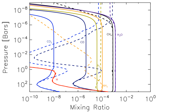
Figure 3.— Effects of vertical mixing on the distributions of H₂O, CH₄, NH₃, N₂, CO, CO₂, and H. The dashed curves are the thermochemical equilibrium profiles for the $\zeta=1$ case from Figure 2 (middle panel). The solid curves are the vertical profiles derived kinetically with only eddy ($K_{zz}=1\times 10^{8}$ cm² s^-1) and molecular diffusion (no photochemistry) using the 1000 bar $\zeta=1$ mixing ratios as the lower boundary condition. Note that kinetically derived profiles begin to match the thermochemical equilibrium profiles at levels below a few 10’s of bars. The rapid fall off of the solid curves near 1 $\mu$bar is due to the sedimentation of the heavier molecules because of molecular diffusion.

In an analogous manner the N₂ quench-level may be calculated by identifying the rate-limiting step in the series of reactions that convert nitrogen to ammonia, and vice versa. These reactions are

$$\rm{H+N_{2}+M\rightarrow N_{2}H+M}$$

$$\rm{H_{2}+N_{2}H\rightarrow N_{2}H_{2}+H}$$

$$\rm{H_{2}+N_{2}H_{2}\rightarrow NH_{2}+NH_{2}}$$

$$\rm{2(H_{2}+NH_{2}\rightarrow NH_{3}+H)}$$

 

$$\rm{Net:4H_{2}+N_{2}\rightarrow 2NH_{3}+2H}$$

In this $\rm{N_{2}\rightleftharpoons NH_{3}}$ sequence R450 is the rate-limiting step, involving the $\rm{N}$ abstraction from diazene, giving a timescale

$$\tau_{chem,\rm{N_{2}}}=\frac{[\rm{N_{2}}]}{k_{450}[\rm{H_{2}}][\rm{N_{2}H_{2}}]}$$ (5)

with reaction rate $k_{450}=2.06\times 10^{-07}T^{-0.93}e^{-20614/T}$, obtained from that of its reverse reaction (Stothard et al. 1995). Calculating $\tau_{chem,\rm{N_{2}}}$ above gives a N₂ quench-level of $\sim$300 bars (see Figure 4), in agreement with the vertical profiles in Figure 3. The abovementioned quench-levels for CO and N₂ are for the adopted eddy diffusion coefficient, $K_{zz}=10^{8}$ cm² s^-1. Increasing $K_{zz}$ to a very large value, $10^{11}$ cm² s^-1, shortens the transport times considerably and increases the quench pressures of CO and N₂ to $\sim 150$ bars and $\sim 620$ bars, respectively. The effects of varying the quench level may be seen in Figure 2 – the atmospheric concentrations of the reservoir gases, CH₄, H₂O and NH₃, and quenched N₂, are relatively insensitive to the location of quench pressure. However, varying the quench-level affects the concentration of CO and CO₂ by orders-of-magnitude.

Vertical dredging of gases leaves a reasonably altered composition in the 1-0.001 bar region, the range of pressure levels wherein the infrared photosphere is located (e.g., Knutson et al. 2009; Swain et al. 2009). For example CO is up to a factor $10^{4}$ more abundant than it would otherwise be. The deep quenching of N bearing gases causes NH₃ to be surprisingly abundant, dominating over the thermochemically favored N₂. In contrast, the largest C and O reservoirs and optically the most active gases, CH₄ and H₂O, are largely unaffected.

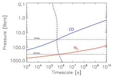
Figure 4.— The blue curve is the CO chemical loss timescale calculated from Equation 4. The red curve is the N₂ chemical loss timescale calculated from Equation 5. The dashed curve is the vertical mixing timescale from Equation 3 using a length scale of $\sim 0.3$H estimated from the Smith et al. (1998) procedure.. The intersection of the vertical mixing timescale and the chemical loss timescale is the quench level for the given species as indicated by the horizontal dotted lines.

3.3. Photochemical Effects

Photochemistry can significantly alter atmospheric composition in the upper portions. The combination of the ultraviolet flux and molecular absorption cross sections gives the photolysis rates for all the species considered here. The altitude of peak production/loss (in units of cm^-3 s^-1), set by the balance between the exponential fall-off of atmospheric density and the inward stellar UV attenuation, occurs near 1 $\mu$bar (this is the well known Chapman function, see Yung & DeMore 1999 pg. 45). Primarily, photolysis breaks apart stable molecules into radicals, which can then react to alter the composition of the upper atmosphere. See Figures 5, 6 and 7 for the photochemically derived mixing ratios. Table 1 compares the column mixing ratios from our models to the observations over the 7 bar to 0.1 bar range probed by the observations. Figure 8 illustrates how photochemistry alters the upper atmosphere. The resultant mixing ratio profiles are compared with those obtained via thermochemical equilibrium (Figure 2), and by vertical mixing (Figure 3).

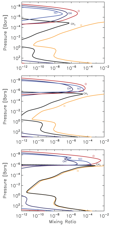
Figure 5.— Mixing ratios for important radicals (OH, NO, O, H, and CH₃) that drive the photochemistry for three metallicities ($\zeta=0.1$(top), $\zeta=1$ (middle), and $\zeta=50$ (bottom)). Note how the CH₃ profile very nearly tracks the H profile because CH₃ is a direct consequence of the oxidation of methane in R60

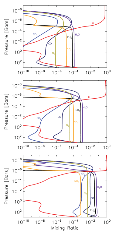
Figure 6.— Photochemically derived mixing ratios for the abundant species (H₂O, CH₄, NH₃, N₂, CO, CO₂, and H) for $\zeta=0.1$ (top), $\zeta=1$ (middle), and $\zeta=50$ (bottom).

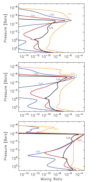
Figure 7.— Photochemically derived mixing ratios for the disequilibrium species, the hydrocarbons and hydrogen cyanide, for $\zeta=0.1$ (top), $\zeta=1$ (middle), and $\zeta=50$ (bottom)

3.3.1 Atomic H & H₂O

Arguably, the most important radical in these atmospheres is atomic hydrogen. Its relatively large abundance ($\sim$75% above 1 $\mu$bar, Figure 6) drives the bulk of disequilibrium chemistry in the upper atmosphere. As is seen in Figures 5-7, when the atomic H abundance increases with altitude, the concentration of disequilibrium species increases with it. Hydrogen attacks the large stable reservoirs, NH₃ and CH₄, to build these desequilibrium species. In the cold Solar System giants, atomic hydrogen is primarily produced by the photosensitized dissociation of H₂ via heavier hydrocarbons, and the photodissociation of CH₄ and ethylene C₂H₄. In hotter giant planets, as in GJ 436b, the atomic hydrogen is made primarily by the photodissociation of water (Liang et al., 2003, Line et al. 2010, Moses et al., 2010). This is because, unlike in the Solar System’s giants, water is not sequestered in clouds and is readily available for photolysis. Its large UV cross section combined with a large thermochemical abundance, makes water the most important source of atomic hydrogen in GJ436b. The detailed mechanism for producing H is the photosensitization of H₂ using water via,

$$\rm{H_{2}O+h\nu\rightarrow OH+H}$$

$$\rm{H_{2}+OH\rightarrow H_{2}O+H}$$

 

$$\rm{Net:H_{2}\rightarrow 2H}$$

This photosensitization is efficient because H₂O dissociates out to $\sim$2000 Å, whereas H₂ dissociates only out to $\sim$800 Å. H₂O acts as a photon sink, with factor $\sim 10^{4}$ more photons available for its photolysis, than for direct H₂ photolysis. Because of these factors the net photosensitized destruction of H₂ by H₂O proceeds 5 orders-of-magnitude faster than the direct photolysis of H₂, and 3 orders-of-magnitude faster than the photosensitized destruction of H₂ via the hydrocarbons. The mixing ratio of water itself is largely unaltered below 1$\mu$bar levels.

3.3.2 CH₄ & Hydrocarbons

Thermochemically, methane is the most abundant hydrocarbon. Overall it is the fourth most abundant species after H₂O, H₂ and He, and it is the parent molecule for the synthesis of all other hydrocarbons. Methane mixing ratios are $\geq 10^{-4}$ at altitudes below the 0.1 mbar level, even for the lowest metallicities. The models generally have methane mixing ratios at least 3 orders-of-magnitude higher than concentrations retrieved from the observations (Madhusudhan & Seager 2011). Although photolysis seems not to significantly modify methane abundances, it does produce large concentrations of the methyl radical, CH₃; this radical is important in the synthesis of heavier hydrocarbons. CH₃ is formed by photosensitized dissociation of methane. The free atomic hydrogen from scheme $III$ readily attacks methane to produce H₂ and CH₃. The trigger and pathway for this is:

$$\rm{H_{2}O+h\nu\rightarrow OH+H}$$

$$\rm{H_{2}+OH\rightarrow H_{2}O+H}$$

$$\rm{H+CH_{4}\rightarrow CH_{3}+H_{2}}$$

 

$$\rm{Net:CH_{4}\rightarrow CH_{3}+H}.$$

The methyl radical’s mixing ratios can be as high as $\sim 10^{-4}$, as in the $\zeta=1$ case (Figure 5). Due to the warmer upper atmosphere, relative to that in the solar system giants, the oxidation of methane (via R60) is more two orders-of-magnitude more efficient than direct photolysis. Because the forward reaction (R60) proceeds more sharply with rising temperature than the reverse (R61), hotter upper atmospheres (as in HD 189733b and HD 209448b) will have a tendency to destroy methane more readily, especially when there are large quantities of photochemically produced atomic hydrogen present. This photosensitized destruction of methane causes it to decline sharply above $\sim$10 $\mu$bars; this is well below the planetary homopause, but well above the infrared photosphere (Figure 8). It also drives the production of heavier hydrocarbons. Little to no heavier hydrocarbon (C_nH_m, where $n,m\geq 2$) is expected via vertical mixing alone, with mixing ratios remaining below $\sim 10^{-10}$ at altitudes above 1 bar. Methane photosensitization (scheme IV) converts the carbon into ethylene (C₂H₄), acetylene (C₂H₂), and ethane (C₂H₆) via

$$\rm{H_{2}O+h\nu\rightarrow OH+H}$$

$$\rm{H_{2}+OH\rightarrow H_{2}O+H}$$

$$\rm{2(H+CH_{4}\rightarrow CH_{3}+H_{2})}$$

$$\rm{CH_{3}+CH_{3}+M\rightarrow C_{2}H_{6}+M}$$

$$\rm{H+C_{2}H_{6}\rightarrow C_{2}H_{5}+H_{2}}$$

$$\rm{H+C_{2}H_{5}\rightarrow C_{2}H_{4}+H_{2}}$$

$$\rm{H+C_{2}H_{4}\rightarrow C_{2}H_{3}+H_{2}}$$

$$\rm{H+C_{2}H_{3}\rightarrow C_{2}H_{2}+H_{2}}$$

 

$$\rm{Net:2CH_{4}+4H\rightarrow C_{2}H_{2}+5H_{2}}$$

The net reaction ultimately produces C₂H₂, making it the most abundant heavy hydrocarbon. This scheme is different than the solar system gas giants where the most dominant pathway for producing acetylene involves the binary collision between two ³CH₂ radicals. This difference can again, be owed to the overwhelming abundance of atomic H from water photolysis which can readily reduce the ethane produced R613 to acetylene. Over the range of metallicities considered ($\zeta=0.1$ to 50), the peak values of C₂ hydrocarbons occur between 10 and 1 $\mu$bars. These mixing ratios of C₂H₄, C₂H₂, C₂H₆ lie between 3$\times$10^-7-6$\times$10^-6, 5$\times$10^-6-4$\times$10^-4, and 5$\times$10^-9-6$\times$10^-5 (Figure 7; for integrated columns see Table 1). For comparison, the peak values in Jupiter are, respectively, $\sim 2\times 10^{-6}$, $5\times 10^{-6}$, and $20\times 10^{-6}$ (Moses et al. 2005). In the Solar System’s giant planets, ethylene, acetylene, and ethane have strong mid-infrared stratospheric emission features at 10.5, 13.7 and 12.1 $\mu$m respectively. These C₂ species can lead to further synthesis of higher order hydrocarbons that can form hydrocarbon aerosols (Zahnle et al. 2009). However, the vapor pressures for these species are high (many bars) at these temperatures, so it may be difficult to form such aerosols. Additionally, Moses et al. 1992 showed that supersaturation ratios of 10 to 1000s may be required in order to trigger condensation due to the lack of nucleation particulates in Jovian type atmospheres.

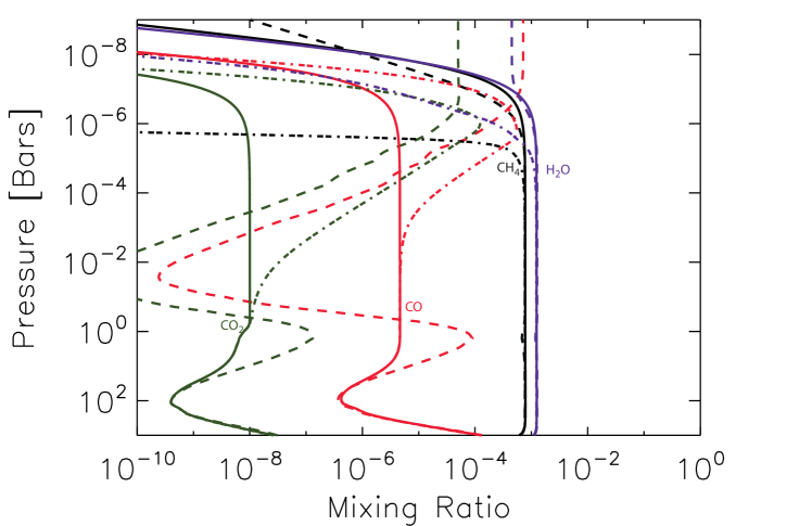
Figure 8.— The effects of vertical mixing and photochemistry compared with the thermochemcial equilibrium profiles for methane, water, carbon monoxide, and carbon dioxide under solar abundances ($\zeta$=1). The dashed curves are the thermochemcially derived mixing ratios (Figure 2 middle panel). The solid curves are the mixing ratios with eddy mixing (as in Figure 3 middle panel). The dot-dashed curves are the photochemical mixing ratios (Figure 5 middle panel). Note that methane becomes photochemically depleted near 1 $\mu$bar when compared to just vertical mixing (solid black curve). CO and CO₂ are photochemically enhanced above the 10 mbar level.

detectability

3.3.3 CO & CO₂

As described in §3.2, the CO abundance above 10 bars is determined by the reaction rate of scheme I, and the strength of vertical mixing. In the absence of incident stellar UV, a profile with a constant vertical mixing ratio up to the homopause is obtained. With incident UV radiation, there is a photochemical enhancement of CO near the 1 $\mu$bar level, of up to a factor of $10^{2}$ for the $\zeta=1$ case (Figure 6, 8). This high altitude enhancement is a property of the cooler atmosphere of GJ 436b; in hot Jupiter atmospheres, as in HD 189733b and HD 209458b, such enhancements or deficits will tend to be driven back towards equilibrium values. The carbon in this extra CO is ultimately derived from the CH₄ reservoir, via the following reaction scheme:

$$\rm{H_{2}O+h\nu\rightarrow OH+H}$$

$$\rm{H_{2}+OH\rightarrow H_{2}O+H}$$

$$\rm{H+CH_{4}\rightarrow CH_{3}+H_{2}}$$

$$\rm{H_{2}O+h\nu\rightarrow O+2H}$$

$$\rm{O+CH_{3}\rightarrow H_{2}CO+H_{2}}$$

$$\rm{H+H_{2}CO\rightarrow HCO+H_{2}}$$

$$\rm{H+HCO\rightarrow CO+H_{2}}$$

 

$$\rm{Net:H_{2}O+CH_{4}\rightarrow CO+2H_{2}+2H}$$

Scheme VI is driven by the water photolysis driven dissociation of CH₄ to CH₃ via scheme IV. Atomic O is produced by photolytic fragmentation of water (R26); the net absorption cross section for this branch is $\simeq 0.1$ that of the main branch in R25. The two radicals, O and CH₃, form formaldehyde in R98, and followed thereafter by a two-step conversion to CO (R233 and R213). An enhancement of CO₂ largely traces the enhancement of CO via:

$$\rm{H_{2}O+h\nu\rightarrow OH+H}$$

$$\rm{OH+CO\rightarrow CO_{2}+H}$$

 

$$\rm{Net:H_{2}O+CO\rightarrow CO_{2}+2H}$$

Photochemically enhanced CO₂ mixing ratios reach $\sim 10^{-4}$ at 1 $\mu$bar for $\zeta=1$. Column averaged mixing ratios are $5\times 10^{-6}$ and $6\times 10^{-9}$ (see Table 1). This is low compared to the observed mixing ratios of $\sim$1$\times$10^-4 and $\sim$1$\times$10^-7, respectively. Increasing the metallicity to $\zeta=50$, increases the mixing ratios to $\sim$1$\times$10^-2 and $\sim$5$\times$10^-4, suggesting that the observed CO and CO₂ columns are consistent with a metallicity enhanced to levels observed in Solar System’s ice giant planets (Table 1).

3.3.4 Nitrogen & HCN

Ammonia and molecular nitrogen, N₂, are thermochemically the two most stable species in a reducing atmosphere and their relative abundance within the $1-0.001$ bar pressure levels is dictated by quench chemistry. Because it is relatively abundant, the addition of hot (quenched or otherwise) NH₃ (Tennyson et al. 2010) to the list of absorbers used for model fitting and retrieval may well be quite important. Other important N species are mainly photochemical byproducts, with HCN being the most abundant photochemically produced molecule between 1 and 0.1 mbar levels, having mixing ratios of typically $10^{-6}$ ($\zeta=1$) to $10^{-5}$ ($\zeta=50$) at 0.1 mbar. Peak HCN occurs well above the photospheric levels, approaching $10^{-4}$ at 1 $\mu$bar. The synthesis of HCN is initiated via water and ammonia photolysis, and completed by subsequent reactions between the ammonia and methane derived radicals:

$$\rm{H_{2}O+h\nu\rightarrow OH+H}$$

$$\rm{H_{2}+OH\rightarrow H_{2}O+H}$$

$$\rm{H+CH_{4}\rightarrow CH_{3}+H_{2}}$$

$$\rm{NH_{3}+h\nu\rightarrow NH_{2}+H}$$

$$\rm{H+NH_{2}\rightarrow NH+H_{2}}$$

$$\rm{NH+CH_{3}\rightarrow CH_{2}NH+H}$$

$$\rm{H+CH_{2}NH\rightarrow H_{2}CN+H_{2}}$$

$$\rm{H+H_{2}CN\rightarrow HCN+H_{2}}$$

 

$$\rm{Net:CH_{4}+NH_{3}\rightarrow HCN+3H_{2}}$$

We note that R43, the photolysis of ammonia to amino radical, is the most important pathway for NH₂ formation at pressures greater than 10 $\mu$bar. At lower pressures this reaction is driven by ammonia photosensitzation,

$$\rm{NH_{3}+H\rightarrow NH_{2}+H_{2}},$$

where the is H derived from H₂O photolysis. In conclusion when water, ammonia and methane are present, disequilibrium HCN is relatively abundant. The best chance for the detection of HCN is via the transmission spectroscopy of its vibrational fundamental bands at 3 and 14 $\mu$m (Shabram et al. 2011).

3.3.5 Sulfur

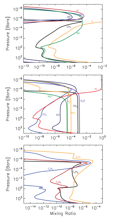
Figure 9.— Photochemically derived mixing ratios for $\zeta=1$ in the presence of sulfur species (H₂S and HS) for the radicals (top), abundant species (middle), and disequilibrium species (bottom). Compare this Figure to the $\zeta=1$ cases in Figures 5, 6, and 7 to see the effects of H₂S on the mixing ratios. Note that the abundance of atomic H is enhanced by orders of magnitude between 1 and 10^-4 bars as a result of scheme IX. This H increase enhances the hydrocarbon abundances significantly in this portion of the atmosphere.

Because atomic H attacks both CH₄ and NH₃, we examine the role of H₂S as a source of free H (Zahnle et al. 2009); S is isoelectronic with and similar in chemical properties to O, but has a considerably reduced primordial abundance, with S/O $\simeq 0.02$. In a subset of models, we introduce the following (very restricted) set of sulfur reactions with accurate laboratory determined reaction rates:

$$\rm{H_{2}S+h\nu\rightarrow SH+H}$$

$$\rm{H_{2}S+H\rightleftharpoons SH+H_{2}}$$

$$\rm{H_{2}S+OH\rightleftharpoons SH+H_{2}O}$$

H₂S is an attractive source of free hydrogen due to its ability to photodissociate out to relative long wavelengths, $\sim$2600 Å. It has a photolysis rate constant comparable to that of H₂O, and we find a $10^{2}$ enhancement in H between the pressure levels of 1 bar and 0.1 mbar upon including these two sulfur species (Figure 9); the relevant reactions are:

$$\rm{H_{2}S+h\nu\rightarrow SH+H}$$

$$\rm{SH+H_{2}\rightarrow H_{2}S+H}$$

 

$$\rm{Net:H_{2}\rightarrow 2H}$$

This enhanced H abundance is catalyzed by the photolysis of H₂S (traced by the SH radical in figure 9, top panel). The atomic H reacts efficiently with CH₄ in R60, producing an increased concentration of the radical CH₃, which in turn drives hydrocarbon production (scheme V) near the 0.1 bar level.

However, the free H in the middle atmosphere, does little to affect the CH₄ mixing ratios; this is because the S/C abundance ratio is low. Sulfur would need to be enriched by a substantial factor of $\sim$20, over the solar S/C value, in order for H₂S to have an appreciable impact on atmospheric CH₄. Although the few considered sulfur species (H₂S, SH) do not much impact the overall chemistry, it is possible that another sulfur compound, such as SO, may act as a catalyst assisting in the conversion of reduced carbon into oxidized carbon. Previously, Moses (1996) has modeled the SL9 Jupiter impact and shown the importance of S in many reaction schemes involving both C and N species, and so the role of S chemistry in the hot extrasolar giants should continue to be investigated in the future (see Zahnle et al. 2009).

Table 1Photochemical model abundances compared with the observations of Stevenson et al. 2010 (S10), Madhusudhan & Seager (2011) (MS10) and Beaulieu et al. (2010) (B10). The model abundances are the integrated column mixing ratios between 7 bars and 0.1 bars, the pressure levels sampled by the observations, for 0.1$\times$, 1$\times$, and 50$\times$ solar elemental abundances.

Molecule	0.1$\times$	1$\times$	50$\times$	MS10	S10	B10
CH4	7.66 $\times$10-05	7.90$\times$10-04	2.96 $\times$10-02	(3-6)$\times$10-06	1$\times$10-07	5$\times$10-04
CO	4.22$\times$10-08	4.29$\times$10-06	8.56$\times$10-03	(3-100)$\times$10-05	(1-7)$\times$10-04	–
CO2	7.74$\times$10-12	6.09$\times$10-09	5.44$\times$10-04	(1-10)$\times$10-07	(1-10)$\times$10-07	–
H2O	1.25$\times$10-04	1.26$\times$10-03	5.09$\times$10-02	$\leq$1$\times$10-03	(3-100)$\times$10-06	–
HCN	4.84$\times$10-10	3.09$\times$10-08	8.41 $\times$10-06	–	–	–
C2H2	1.21$\times$10-14	1.18$\times$10-12	2.10 $\times$10-09	–	–	–
NH3	1.45$\times$10-05	1.06$\times$10-04	6.54$\times$10-04	–	–	–
H2S	–	$3.22\times$10-05	–	–	–	–

4. Discussion & Conclusions

We have developed a 1D “thermochemical and photochemical kinetics with transport” model following Visscher et al. (2010) and recently, Moses et al. (2011) for extrasolar planet atmospheres. We use a compilation of bidirectional reactions of the five most abundant elements to model both the equilibrium and disequilibrium portions of the atmosphere. Using detailed balance with both forward and reverse reactions, allows our model to reach thermochemical equilibrium kinetically, thereby obviating the need to choose ad hoc lower boundaries for multiple quenched species, and allowing a seamless transition between the transport dominated and the chemical equilibrium zones. A limitation is that we adopt a static temperature structure; a future improvement would allow the iterative adjustment and co-evolution of the temperature structure with the chemistry. Also, the eddy diffusivity profile $K_{zz}(z)$ is poorly constrained, and is essentially a free parameter in any of these models.

We have applied our models to study the atmosphere of the transiting Neptune-like planet GJ 436b. The elemental abundance of atmosphere, a key input parameter, is relatively uncertain, but mass-radius constraints suggest that GJ 436b must be enriched to at least $10\times$ solar levels. We model a range of atmospheric enrichment to cover this instrinsic uncertainty; we observe the trends when varying $\zeta$, and rule out the possibility that intermediate values of $\zeta$ would spring any surprises. The UV fluxes of stars other than the Sun are often difficult to obtain. M-dwarf hosts can be chromospherically hyperactive, and because UV photolysis may drive the depletion of weakly bonded molecules such as CH₄, NH₃ and H₂S, it is important to have an accurate UV estimate for GJ 436. We use a combination of GALEX and HST UV fluxes along with Rosat and XMM-Newton soft X-ray fluxes to bound the UV continuum and line emission of GJ 436.

The GJ 436b model atmospheres show that a combination of photochemistry, chemical kinetics and transport-induced quenching drives the composition well out of equilibrium. While equilibrium conditions are maintained in the deep, hot, troposphere (below a 10s of bars for $\rm CO\rightleftharpoons CH_{4}$, and 100s of bars for $\rm N_{2}\rightleftharpoons NH_{3}$), the composition of the middle atmosphere is altered by the dredging up of quenched gases such as CO and NH₃. The effects of transport disequilibrium are prominent in cooler planets such as GJ 436b because the quench points for major species depend on the temperature. As it gets colder, the pressure points for quenching are pushed deeper into the atmosphere due to the longer interconversion timescales from one species reservoir to another. In contrast to the quenched species (CO, CO₂, NH₃), the effect of vertical mixing on the reservoir gases such as CH₄ and H₂O is relatively feeble.

The reservoir gases H₂O and CH₄, and NH₃ are largely unaffected by photochemistry because of their (a) large abundances, and (b) rapid recycling. Nevertheless, it is their photolysis that drives the bulk of the disequilibrium chemistry in the upper atmosphere producing CH₄ and NH₃ sinks such as heavier hydrocarbons (such as C₂H₂, etc.) and simple nitriles (such as HCN). Much as in the hot Jupiters (Liang et al. 2003), H is the most important and active atom in the bulk of the atmosphere; it is created by the photosensitized destruction of H₂, catalyzed by the presence of H₂O and H₂S. The latter gas, though less abundant than water, is important because of its ability to capture incident starlight photons out wavelengths as long as $2600$ Å. In most models, H replaces H₂ as the most abundant species in the atmosphere above the planetary homopause at $\simeq 1$ $\mu$bar. Because CH₄ is the largest C carrier in the planet’s UV photosphere, we create abundant C₂ compounds (Figure 7) despite the relatively efficient hydrogenation back to CH₄. Species such as acetylene, C₂H₂, formed in abundance in our enriched models, are precursors for potential hydrocarbon soot formation in the upper atmosphere (as opposed to the hotter Jupiters such as HD 209458b and HD 189733b, wherein CO carries the bulk of carbon in the stratosphere). Our reaction lists for hyrdocarbon chemistry are truncated at C₂, and so we do not synthesize C₃ and heavier hydrocarbons and nitriles explicitly.

Within the range physical and chemical processes captured in our models, and the considered reaction sets and their kinetics, we find it difficult explain the observations suggesting a methane-poor GJ 436b. Except above 1 $\mu$bar pressure levels where CH₄ is photochemically converted to CO, HCN and C₂ hydrocarbons, it remains the predominant C reservoir in the lower atmosphere and in the region of the IR photosphere. The observed abundances of quenched CO and CO₂ are in agreement with an atmosphere enriched to levels intermediate between 1 to 50 times solar (as in Madhusudhan & Seager 2011). The depleted water may either contrarily suggest a sub solar metallicity (Table 1), or skewed heavy metals ratios; the latter is a possibility which we have not considered herein as there are far too many combinations to explore. In the 1$\times$ solar models, the methane abundance is consistent with the values retrieved by Beaulieu et al. (2010) (Table 1) using transit observations. We suppose it is possible that a more complete inclusion of other relatively abundant elements such as S and P, or distorted elemental ratios (C/O or O/S etc.), or ill-understood chemistry and exotic processes (not considered herein, such as the 3 dimensionality of the problem) could do more to explain the chemistry of this enigmatic atmosphere.

We agree with Moses et al. (2011) that quench level arguments can be used to predict abundances, so long as this is done with the appropriate level of caution. By this, we mean that the relevant rate-limiting reaction must necessarily be identified in order to properly calculate the timescale for chemical loss. Also, quenched gases do not share a common quench level and assuming so can result in gross under- or overestimation of their abundances. For example, as shown herein, N₂ and CO have vastly different quench levels. For the moderate to high levels of incident UV flux, photolysis generates high concentrations of secondary byproducts, but does not significantly alter the abundances of the reservoir gases; in our estimation photochemistry cannot alter the dayside methane budget. Hotter atmospheres with sluggish vertical mixing and hot stratospheres are required for severe methane depletion. For example, in figure 10, we approximate such as atmosphere as isothermal with $T=1200$ K, $\zeta=5$, and $K_{zz}$=$1\times 10^{6}$ cm²s^-1, and with zero UV irradiation (similar to models by Zahnle et al. 2009). In this hypothetical atmosphere there is relatively little quenched methane. At $T=1200$ K and low pressures, the rate determining step for CH₄ $\rightarrow$ CO (reverse of R351) is faster than the vertical transport time throughout the atmosphere, allowing the CH₄ to be in thermochemical equilibrium with CO everywhere (Figure 10). Since equilibrium conditions apply, the $P^{2}$ term in equation 2 results in the rapid vertical fall-off of CH₄.

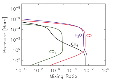
Figure 10.— Mixing ratios for, CO, CH₄, CO₂, and H₂O assuming a T=1200 K isothermal atmosphere, $\zeta=5$, and $K_{zz}$=$1\times 10^{6}$ cm²s^-1, with no photochemistry. The observed methane fall-off is due to high temperatures alone; high temperatures imply a short chemical loss time for of CH₄. Because of the large transport time, CH₄ and CO are nearly in equilibrium at all altitudes.

The models presented herein are by no means restricted in applicability to GJ 436b like Neptunes, and much of the modeled chemical state may be generalized to H/He dominated planets in the 500-1000 K temperature range. In this regime CH₄ is the primary carbon carrier and CO is quenched. The reverse is true in hotter atmospheres, $T>10^{3}$ K, where CO is the primary carbon carrier and CH₄ is quenched. NH₃ is quenched deep in the atmosphere and can be quite abundant in the photosphere. Higher hydrocarbons and HCN are produced photochemically in relatively high abundances at mbar to $\mu$bar pressures. Similarly, an enhancement of CO and CO₂ over the quench concentrations, driven by the photolysis of H₂O, is observed in the high atmosphere. Water is in gaseous phase and abundant, and not condensed out as it would be in cooler atmospheres. GJ 1214b, a $T\simeq 500$ K low super Earth or mini Neptune, also orbiting an M dwarf primary (Charbonneau et al. 2009; Sada et al. 2010; Bean et al. 2010; Carter et al. 2011; Désert et al. 2011), falls in this regime of warm atmospheres. If GJ 1214b is in possession of a reducing H-He atmosphere (Croll et al. 2011; Crossfield et al. 2011), much of the atmospheric chemistry would be analogous to that in GJ 426b; this, however, is speculative as there is much current debate over the bulk composition of GJ 1214b.

5. Acknowledgements

We would like to thank Julie Moses, Channon Visscher, Karen Willacy, and M.C. Liang for useful chemistry discussions and tips. We would also like to thank Xi Zhang, Heather Knutson, Mimi Gerstell, Mark Allen, the Yuk Yung Group, and the anonymous referee for reading the manuscript and providing valuable feedback. M. Line is supported by the JPL Graduate Fellowship funded by the JPL Research and Technology Development Program. P. Chen & G. Vasisht are supported by the JPL Research & Technology Development Program, and contributions herein were supported by the Jet Propulsion Laboratory, California Institute of Technology, under a contract with the National Aeronautics and Space Administration.

References

- Allen et al. (1981) Allen, M., Yung, Y. L., & Waters, J. W. 1981, J. Geophys. Res., 86, 3617
- Anders et al. (1982) Anders, E. & Ebihara, M., 1981, Geochem. Cosmo. Chem. Acta., 46, p. 2363
- Asplund et al. (2009) Asplund, M., Grevesse, N., Sauval, A. J., & Scott, P. 2009, ARA&A, 47, 481
- Batygin et al. (2009) Batygin, K., Laughlin, G., Meschiari, S., Rivera, E., Vogt, S., & Butler, P. 2009, ApJ, 699, 23
- Bean et al. (2006) Bean, J. L., Benedict, G. F., & Endl, M. 2006, ApJ, 653, L65
- Bean et al. (2010) Bean, J. L., Kempton, E. M.-R., & Homeier, D. 2010, Nature, 468, 669
- Beaulieu et al. (2011) Beaulieu, J.-P., et al. 2011, ApJ, 731, 16
- Butler et al. (2004) Butler, R. P., Vogt, S. S., Marcy, G. W., Fischer, D. A., Wright, J. T., Henry, G. W., Laughlin, G., & Lissauer, J. J. 2004, ApJ,617, 580
- Carter et al. (2011) Carter, J. A., Winn, J. N., Holman, M. J., Fabrycky, D., Berta, Z. K., Burke, C. J., & Nutzman, P. 2011, ApJ, 730, 82
- Charbonneau et al. (2009) Charbonneau, D., et al. 2009, Nature, 462, 891
- Chase et al. (1985) Chase Jr, M.W. & Davies, C. 1985, J. Phys. Chem. Ref. Data, 14, 1856
- Croll et al. (2011) Croll, B., Albert, L., Jayawardhana, R., Miller-Ricci Kempton, E., Fortney, J. J., Murray, N., & Neilson, H. 2011, arXiv:1104.0011
- Crossfield et al. (2011) Crossfield, I. J. M., Hansen, B. M. S., & Barman, T. 2011, arXiv:1104.1173
- Cooper & Showman (2006) Cooper, C. S., & Showman, A. P. 2006, ApJ, 649, 1048
- Doyle et al. (1997) Doyle, J. G., Mathioudakis, M., Andretta, V., Short, C. I., & Jelinsky, P. 1997, A&A, 318, 835
- Deming et al. (2007) Deming, D., Harrington, J., Laughlin, G., Seager, S., Navarro, S. B., Bowman, W. C., & Horning, K. 2007, ApJ, 667, L199
- Désert et al. (2011) Désert, J.-M., et al. 2011, ApJ, 731, L40
- Ehrenreich et al. (2011) Ehrenreich, D., Lecavelier Des Etangs, A., & Delfosse, X. 2011, A&A, 529, A80
- Figueira et al. (2009) Figueira, P., Pont, F., Mordasini, C., Alibert, Y., Georgy, C., & Benz, W. 2009, A&A, 493, 671
- Gillon et al. (2007) Gillon, M., Pont, F., Demory, B. O., Mallmann, F., Mayor, M., Mazeh, T., Queloz, D., Shporer, A., Udry, S., & Vuissoz, C. 2007, 472, L13
- Gizis et al. (2002) Gizis, J. E., Reid, I. N., & Hawley, S. L. 2002, AJ, 123, 3356
- Gladstone et al. (1996) Gladstone, G. R., Allen, M., & Yung, Y. L. 1996, Icarus, 119, 1
- Gordon & McBride. (1996) Gordon, S., McBride, B.J., & NASA Tech. Info. Program, 1996, Computer program for calculation of complex chemical equilibrium compositions and applications, National Aeronautics and Space Administration, Office of Management, Scientific and Technical Information Program
- Griffith & Yelle (1999) Griffith, C. A., & Yelle, R. V. 1999, ApJ, 519, L85
- Gurvich et al. (1989) Gurvich, L.V. and Veyts, IV and Alcock, CB, institut prikladno khimii (Soviet Union) 1989, Thermodynamic properties of individual substances, Hemisphere Publisher
- Hubeny & Burrows (2007) Hubeny, I., & Burrows, A. 2007, ApJ, 669, 1248
- Hünsch et al. (1999) Hünsch, M., Schmitt, J. H. M. M., Sterzik, M. F., & Voges, W. 1999, A&AS, 135, 319
- Jodkowski et al. (1999) Jodkowski, J.T. and Rayez, M.T. and Rayez, J.C. and Bérces, T. and Dóbé, S. 1999, J. Phys. Chem. A., 103, 3750
- Knutson et al. (2009) Knutson, H. A., et al. 2009, ApJ, 690, 822
- Kramm et al. (2011) Kramm, U., Nettelmann, N., Redmer, R., & Stevenson, D. J. 2011, A&A, 528, A18
- Landsman & Simon (1993) Landsman, W., & Simon, T. 1993, ApJ, 408, 305
- Lewis et al. (2010) Lewis, N. K., Showman, A. P., Fortney, J. J., Marley, M. S., Freedman, R. S., & Lodders, K. 2010, ApJ, 720, 344
- Liang et al. (2003) Liang, M.-C., Parkinson, C. D., Lee, A. Y.-T., Yung, Y. L., & Seager, S. 2003, ApJ, 596, L247
- Liang et al. (2004) Liang, M.-C., Seager, S., Parkinson, C. D., Lee, A. Y.-T., & Yung, Y. L. 2004, ApJ, 605, L61
- Line et al. (2010) Line, M. R., Liang, M. C., & Yung, Y. L. 2010, ApJ, 717, 496
- Lodders (2002) Lodders, K. 2002, ApJ, 577, 974
- Mardling (2008) Mardling, R. A. 2008, arXiv:0805.1928
- Moses (1996) Moses, J. I. 1996, IAU Colloq. 156: The Collision of Comet Shoemaker-Levy 9 and Jupiter, 243
- Moses et al. (1992) Moses, J. I., Allen, M., & Yung, Y. L. 1992, Icarus, 99, 318
- Moses et al. (2005) Moses, J. I., Fouchet, T., Bézard, B., Gladstone, G. R., Lellouch, E., & Feuchtgruber, H. 2005, Journal of Geophysical Research (Planets), 110, 8001
- Moses et al. (2011) Moses, J. I., et al. 2011, arXiv:1102.0063
- Nettelmann et al. (2010) Nettelmann, N., Kramm, U., Redmer, R., & Neuhäuser, R. 2010, A&A, 523, A26
- Prinn & Barshay (1977) Prinn, R. G., & Barshay, S. S. 1977, Science, 198, 1031
- Ribas et al. (2008) Ribas, I., Font-Ribera, A., & Beaulieu, J.-P. 2008, ApJ, 677, L59
- Rogers & Seager (2010) Rogers, L. A., & Seager, S. 2010, ApJ, 716, 1208
- Sada et al. (2010) Sada, P. V., et al. 2010, ApJ, 720, L215
- Sanz-Forcada et al. (2010) Sanz-Forcada, J., García-Álvarez, D., Velasco, A., Solano, E., Ribas, I., Micela, G., & Pollock, A. 2010, Pathways Towards Habitable Planets, 430, 530
- Shabram et al. (2011) Shabram, M., Fortney, J. J., Greene, T. P., & Freedman, R. S. 2011, ApJ, 727, 65
- Showman et al. (2009) Showman, A. P., Fortney, J. J., Lian, Y., Marley, M. S., Freedman, R. S., Knutson, H. A., & Charbonneau, D. 2009, ApJ, 699, 564
- Smith (1998) Smith, M. D. 1998, Icarus, 132, 176
- Stevenson et al. (2010) Stevenson, K. B., et al. 2010, Nature, 464, 1161
- Stothard et al. (1995) Stothard, N. and Humpfer, R. and Grotheer, H.H., 1995, Chem. Phys. Lett., 240, 474
- Saumon et al. (2007) Saumon, D., et al. 2007, ApJ, 656, 1136
- Saumon et al. (2006) Saumon, D., Marley, M. S., Cushing, M. C., Leggett, S. K., Roellig, T. L., Lodders, K., & Freedman, R. S. 2006, ApJ, 647, 552
- Saumon et al. (2003) Saumon, D., Marley, M. S., & Lodders, K. 2003, arXiv:astro-ph/0310805
- Swain et al. (2009) Swain, M. R., Vasisht, G., Tinetti, G., Bouwman, J., Chen, P., Yung, Y., Deming, D., & Deroo, P. 2009, ApJ, 690, L114
- Tennyson (2010) Tennyson, J. 2010, European Planetary Science Congress 2010, held 20-24 September in Rome, Italy. ¡A href=”http://meetings.copernicus.org/epsc2010”¿http://meetings.copernicus.org/epsc2010¡/A¿, p.172, 172
- Torres et al. (2008) Torres, G., Winn, J. N., & Holman, M. J. 2008, ApJ, 677, 1324
- Visscher et al. (2010) Visscher, C., Moses, J. I., & Saslow, S. A. 2010, Icarus, 209, 602
- Walkowicz et al. (2008) Walkowicz, L. M., Johns-Krull, C. M., & Hawley, S. L. 2008, ApJ, 677, 593
- Woods et al. (2004) Woods, P. M., et al. 2004, ApJ, 605, 378
- Wright et al. (2011) Wright, J. T., et al. 2011, ApJ, 730, 93
- Yung & Demore (1999) Yung, Y. L., & Demore, W. B. 1999, Photochemistry of planetary atmospheres / Yuk L. Yung, William B. DeMore. New York : Oxford University Press, 1999. QB603.A85 Y86 1999
- Yung et al. (1988) Yung, Y. L., Drew, W. A., Pinto, J. P., & Friedl, R.R. 1988, Icarus, 73, 516
- Zahnle et al. (2009) Zahnle, K., Marley, M. S., & Fortney, J. J. 2009, arXiv:0911.0728
- Zahnle et al. (2009) Zahnle, K., Marley, M. S., Freedman, R. S., Lodders, K., & Fortney, J. J. 2009, ApJ, 701, L20
- Zehe et al. (2001) Zehe, M.J. and Gordon, S. and McBride, B.J. 2001, CAP: a computer code for generating tabular thermodynamic functions from NASA lewis coefficients, National Aeronautics and Space Administration, Glenn Research Center