The Adams-Bashforth-Moulton Integration Methods Generalized to an Adaptive Grid

Abstract

We present a generalization of the Adams-Bashforth-Moulton predictor-corrector numerical integration methods to an adaptive grid. The step size may be chosen dynamically in order to maintain a desired relative magnitude of error in each step. We demonstrate that the methods remain convergent to the expected degree, and apply various methods to the famous problem of determining the maximum possible mass of a neutron star supported by pure fermionic exclusion pressure. We reproduce the Tolman-Oppenheimer-Volkoff result of 0.71 solar masses using only 23 integration steps, and reproducing both mass and radius within 1% requires 27. We also present various optimizations and features of our implementation.

1 INTRODUCTION

The Adams-Bashforth (AB) family of integration methods (Bashforth and Adams, 1883) are explicit, linear, multistep techniques. Each successive member of the family has a higher order of convergence, and the family can be extended indefinitely. The Adams-Moulton (AM) family of integration methods (Moulton, 1926) are, similarly, implicit, linear, multistep techniques, and can be similarly extended to arbitrarily high order of convergence. Combining the two allows the use of an Nth order, AB method’s explicit result for an integration step as a prediction to be inserted into the AM method of order N+1, thereby achieving a next-order correction for the integration step, as well as an estimate of the error in that step. We will term this predictor-corrector combined method Adams-Bashforth-Moulton. For clarity, we will refer to the orders of convergence of both the Adams-Bashforth predictor phase and the Adams-Moulton correction phase, e.g. “ABM fixed-grid method of order 3-4.”

The principle of traditional, fixed-grid AB and AM methods is to integrate analytically a Lagrange interpolating polynomial fit to various previous values of the derivative. Each successive integration step is thereby reduced to a fixed weighted average of some number of the previous (and for AM methods, one future/predicted) derivative data points. For fixed step size, the fit and integration can be done ahead of time, once, and apply to all mesh locations, for all variables to be integrated and all integration steps.

The fixed-grid AB and AM methods can be combined, but then the error estimate is a passive report useful only in ex post facto analysis. The adaptive-grid methods we present here use the error estimate dynamically, to adjust the step size. They still allow a set of weighting factors to be used in all mesh locations and for all variables. However, the weights must be recalculated with each new integration step. Happily, the computational overhead demanded by our methods is negligible compared to derivative evaluation for complex problems, especially as it does not scale with the size of the mesh or number of variables to be integrated.

The AB and AM methods having been derived in the nineteenth century (Bashforth and Adams, 1883), their fixed weighting was customarily used to reduce the computational overhead of each step. In a twenty-first century context, however, maintaining fixed weights (and thus a fixed step size) amounts to assuming that the derivatives are extremely computationally inexpensive. This assumption is massively violated for nearly all simulations done today; for instance, in radiation transport, unless potentially hazardous simplifying assumptions are made, the radiation field is a function of seven independent variables $\left(x,y,z,\theta,\phi,\nu,t\right)$, i.e., spatial location, two angles to specify direction, frequency, and time. Since the first six dimensions must be solved for every derivative evaluation, this dominates the computational time required for a radiation transport-hydrodynamics simulation.

Because of the working assumption of cheap derivatives and the handicap of fixed step size, we believe the AB and AM methods have been neglected by the simulation community in favor of methods such as Runge-Kutta (RK) (Runge, 1895). The RK methods can be used in an implicit scheme and allow an adaptive step size, at the unfortunate price of even more derivative evaluations per integration step, increasing with the order of convergence of the particular method selected. In the case of the most commonly used RK method, the explicit fourth order Runge-Kutta, this means derivatives must be evaluated four times for each integration step.

The adaptive mesh ABM methods presented here embody a highly advantageous combination of features. These methods require only two derivative evaluations per integration step (independent of convergence order!), are implicit and therefore avoid Courant-Friedrichs-Lewy conditioning (Courant, Friedrichs, and Lewy, 1928), provide arbitrarily high orders of convergence, and use the error estimate afforded by combining the AB and AM methods to maintain an approximately constant fractional error through each integration step. The last three features in concert allow the size of the integration step to be, potentially, extremely large. Two derivative evaluations per integration step is the minimum possible for an implicit scheme, as implicity requires knowledge of at least the derivative at the present value of the independent variable and at the next data point for which the method is implicitly solving.

The price extracted for the speed-ups just mentioned are that previous values of the derivatives must remain accessible to the integration routine. Codes that use single, rather than multi-step integration methods methods may write their meshes to file (to be archived and never touched by the code again) and then alter the mesh in place. These codes would have to be rewritten in order to maintain code access to roughly as many integration steps as the desired order of convergence. We believe any penalty in either memory requirements or hard disk lag will be far outweighed by the speed-ups the ABM methods make achievable for problems in which derivative evaluation is very expensive.

Another pitfall to be avoided is Runge’s phenomenon (Runge, 1901), where the error involved in an interpolation actually increases as the order of the interpolating polynomial becomes very large, due to a “ringing” effect. The order of convergence can be tuned for a particular problem in order to minimize Runge’s phenomenon. We demonstrate this tuning in Section 4.5, where we find the order of convergence that requires the fewest integration steps for a particular prescribed precision.

We explore the practical application of our ABM methods with a trial problem of determining the Tolman-Oppenheimer-Volkoff (TOV) limit (Tolman, 1934) for the Oppenheimer-Volkoff (OV) equation of state (Oppenheimer and Volkoff, 1939).

2 THEORY

2.1 Adams-Bashforth

Our methods represent a discretization of the quantity we wish to integrate numerically. Let us call the function we would like to calculate and its derivative, respectively, $y\left(x\right)$ and $y^{\prime}\left(x\right)$. In complete generality we can quantize it thus:

$$y_{i+1}\equiv y\left(x_{i+1}\right)=y\left(x_{i}\right)+\int_{x_{i}}^{x_{i+1}}y^{\prime}\left(x,y\right)\,\mathrm{d}x$$ (1)

We shall quantize the derivative and other quantities with Latin letter subscripts analogously, and call the initial conditions $y_{0}\equiv y(x_{0})$. Note that multiple variables, coupled or not, can be integrated by giving $y$ and $y^{\prime}$ vector subscripts, as well. This subscript can denote either a true, traditional vector, or simply a list of variables all needing integration (e.g., $m$ and $P$, as will be discussed in Section 4). For simplicity, we omit any such subscript in the following derivation.

The Adams-Bashforth methods are based on a Lagrange polynomial approximation to the derivative. Our method requires a new Lagrange polynomial at each integration step $i$, which we shall call $P_{\mathrm{AB}\,i}$. For an order of convergence $N$, we have:

$$P_{\mathrm{AB}\,i}\left(\bar{x}\right)\equiv\sum_{j=i-N+1}^{i}y^{\prime}_{j}\prod_{k=i-N+1,k\neq j}^{i}\frac{\left(\bar{x}-x_{k}\right)}{\left(x_{j}-x_{k}\right)}$$ (2)

where $y^{\prime}_{j}=y^{\prime}\left(x_{j},y_{j}\right)$. Choosing $\bar{x}=x-x_{i}$ allows us to identify the origin according to $P_{\mathrm{AB}\,i}$ with the most recent integration step. Our analysis is simplified if we make the following definition:

$$\psi_{\mathrm{AB}\,ij}\left(\bar{x}\right)\equiv\prod_{k=i-N+1,k\neq j}^{i}\frac{\left(\bar{x}-x_{k}\right)}{\left(x_{j}-x_{k}\right)}$$ (3)

Thus:

$$P_{\mathrm{AB}\,i}\left(\bar{x}\right)=\sum_{j=i-N+1}^{i}y^{\prime}_{j}\psi_{\mathrm{AB}\,ij}\left(\bar{x}\right)$$ (4)

With this definition in hand, we can now derive our Adams-Bashforth approximation to $y_{i+1}$. With our earlier selection of the origin of $P_{\mathrm{AB}\,i}$, the integral in Equation 1 becomes:

$$y_{\mathrm{AB}\,i+1} \approx y_{\mathrm{AB}}\left(x_{i}\right)+\int_{0}^{\Delta x_{i}}P_{\mathrm{AB}\,i}\left(\bar{x}\right)\,\mathrm{d}\bar{x}$$

$$= y_{\mathrm{AB}}\left(x_{i}\right)+\int_{0}^{\Delta x_{i}}\sum_{j=i-N+1}^{i}y^{\prime}_{j}\psi_{\mathrm{AB}\,ij}\left(\bar{x}\right)\,\mathrm{d}\bar{x}$$

$$= y_{\mathrm{AB}}\left(x_{i}\right)+\sum_{j=i-N+1}^{i}\left(\int_{0}^{\Delta x_{i}}\psi_{\mathrm{AB}\,ij}\left(\bar{x}\right)\,\mathrm{d}\bar{x}\right)y^{\prime}_{j}$$

Note that $\psi_{\mathrm{AB}\,ij}\left(\bar{x}\right)$ is a calculable polynomial and can be integrated analytically. We implement that analytic integration with the following definitions:

$$\Phi_{\mathrm{AB}\,i}\left(\bar{x}\right)\equiv\prod_{k=i-N+1}^{i}\left(\bar{x}-x_{k}\right)$$ (6)

and

$$\phi_{\mathrm{AB}\,ij}\left(\bar{x}\right)\equiv\prod_{k=i-N+1,k\neq j}^{i}\left(\bar{x}-x_{k}\right)=\frac{\Phi_{\mathrm{AB}\,i}\left(\overline{x}\right)}{\left(\overline{x}-x_{j}\right)}$$ (7)

We use an equals sign loosely in Equation 7 because the rightmost expression is undefined for $\overline{x}=x_{j}$ while the middle expression has no such singularity. This is immaterial to us, however, as we will evaluate the fraction analytically before substituting in any specific values for variables. Using an equals sign in a similar way, we can therefore express $\psi_{\mathrm{AB}\,ij}\left(\bar{x}\right)$ as:

$$\psi_{\mathrm{AB}\,ij}\left(\overline{x}\right)=\frac{\phi_{\mathrm{AB}\,ij}\left(\overline{x}\right)}{\phi_{\mathrm{AB}\,ij}\left(x_{j}\right)}$$ (8)

If we compute the product $\Phi_{\mathrm{AB}\,i}\left(\bar{x}\right)$ first and save the penultimate intermediate result, we need calculate only the product of $N$ binomials and carry out $N-1$ synthetic polynomial divisions of that product by binomials for each integration step.

2.2 Adams-Moulton

The derivation of the AM methods proceeds almost identically to the AB methods, so we present them with little comment. Note that the upper boundary of the sums and products in these equations is $i+1$, in contrast to the $i$ limit of the AB method formulae.

$$P_{\mathrm{AM}\,i}\left(\bar{x}\right)\equiv\sum_{j=i-N+1}^{i+1}y^{\prime}_{j}\prod_{k=i-N+1,k\neq j}^{i+1}\frac{\left(\bar{x}-x_{k}\right)}{\left(x_{j}-x_{k}\right)}$$ (9)

The key to linking the AB and AM methods into an ABM predictor-corrector tandem is to insert the AB prediction for $y_{i+1}$ into the calculation of $y^{\prime}_{i+1}$. That is,

$$y^{\prime}_{i+1}\equiv y^{\prime}\left(x_{i+1},y_{\mathrm{AB}\,i+1}\right)$$ (10)

With this identification, the derivation proceeds as before.

$$\psi_{\mathrm{AM}\,ij}\left(\bar{x}\right)\equiv\prod_{k=i-N+1,k\neq j}^{i+1}\frac{\left(\bar{x}-x_{k}\right)}{\left(x_{j}-x_{k}\right)}$$ (11)

$$P_{\mathrm{AM}\,i}\left(\bar{x}\right)\equiv\sum_{j=i-N+1}^{i+1}y^{\prime}_{j}\psi_{\mathrm{AM}\,ij}\left(\bar{x}\right)$$ (12)

$$y_{\mathrm{AM}}\left(x_{i+1}\right) \approx y_{\mathrm{AM}}\left(x_{i}\right)+\int_{0}^{\Delta x_{i}}P_{\mathrm{AM}\,i}\left(\bar{x}\right)\,\mathrm{d}\bar{x}$$

$$= y_{\mathrm{AM}}\left(x_{i}\right)+\int_{0}^{\Delta x_{i}}\sum_{j=i-N+1}^{i+1}y^{\prime}_{j}\psi_{\mathrm{AM}\,ij}\left(\bar{x}\right)\,\mathrm{d}\bar{x}$$

$$= y_{\mathrm{AM}}\left(x_{i}\right)+\sum_{j=i-N+1}^{i+1}\left(\int_{0}^{\Delta x_{i}}\psi_{\mathrm{AM}\,ij}\left(\bar{x}\right)\,\mathrm{d}\bar{x}\right)y^{\prime}_{j}$$

We implement the calculation in a similar fashion as well.

$$\Phi_{\mathrm{AM}\,i}\left(\bar{x}\right)\equiv\prod_{k=i-N+1}^{i+1}\left(\bar{x}-x_{k}\right)$$ (14)

$$\phi_{\mathrm{AM}\,ij}\left(\bar{x}\right)\equiv\prod_{k=i-N+1,k\neq j}^{i+1}\left(\bar{x}-x_{k}\right)=\frac{\Phi_{\mathrm{AM}\,i}\left(\overline{x}\right)}{\left(\overline{x}-x_{j}\right)}$$ (15)

$$\psi_{\mathrm{AM}\,ij}\left(\overline{x}\right)=\frac{\phi_{\mathrm{AM}\,ij}\left(\overline{x}\right)}{\phi_{\mathrm{AM}\,ij}\left(x_{j}\right)}$$ (16)

Ordinarily, the AB and AM methods require some other method, such as RK, initially to supply enough derivative points to allow the use of the desired order of method. These methods are designed to maintain a particular precision, so instead we have implemented a boot-strapping technique, where $y_{0}$ is supplied as the boundary condition, $y_{1}$ is calculated using a first-order AB and second-order AM method, $y_{2}$ is calculated using a second- and third-order tandem, etc., until enough data points have been calculated that we can proceed with the desired method. This can be elegantly implemented by replacing the lower limits of sums and products with zero when they would be negative. We will explore the consequences of this technique in Section 3

For a production-quality data run, the step sizes need only be chosen small enough that the desired precision is maintained throughout the bootstrapping phase.

2.3 Selecting A Step Size

For most purposes, it is the precision of the final answer, not the specific number of steps or specific step size that is of interest. The power of an explicit-implicit predictor-corrector method is that it allows the integrator to maintain an approximately constant relative size of correction term throughout an integration. The user of the technique we present, therefore, can specify the desired precision of integration directly. In this section, we demonstrate how.

The two phases of a tandem ABM method of orders $N$ and $N+1$ estimate the quantity to be integrated with orders of convergence that differ by one. Subtracting the two estimates therefore gives a correction term of order $N+1$ in the step size. Dividing by the prediction gives the fractional or relative correction:

$$\epsilon_{i}=\frac{y_{\mathrm{AM}\,i+1}-y_{\mathrm{AB}\,i+1}}{y_{\mathrm{AB}\,i+1}}\propto O\left(\Delta x_{i}^{N+1}\right)$$ (17)

Let us call the constant of proportionality in the above relation $k_{i}$. We then find that:

$$\frac{\epsilon_{i+1}}{\epsilon_{i}}=\frac{k_{i+1}}{k_{i}}\left(\frac{\Delta x_{i+1}}{\Delta x_{i}}\right)^{N+1}$$ (18)

If we desire an ordained fractional correction of $E$ in each integration step, let us simply set $\epsilon_{i+1}=E$ in Equation 18. We thereby derive a prescription for the next step size:

$$\Delta x_{i+1}=\left(\sqrt[N+1]{\frac{Ek_{i}}{\epsilon_{i}k_{i+1}}}\right)\Delta x_{i}$$ (19)

Without additional evaluations of the derivative, we do not have any means of estimating the ratio $k_{i}/k_{i+1}$. Evaluating additional derivatives would, of course, defeat the purpose of the methods we are presenting, so instead let us observe that the ratio enters into the prescription for the next step size only inside a root that in practice may be as high as 9${}^{\text{th}}$ or 10${}^{\text{th}}$, as we will see in Section 4. Assuming that the ratio is unity will typically result in only small changes in $\Delta x$ from one step to the next. Furthermore, adjusting the step size with every integration step allows the method to continue adapting to a transiently large ratio over a few integration steps. In addition, it may be possible for the derivative evaluation procedures themselves to detect regimes where the ratio is likely to deviate more from unity, such as near phase changes, and to signal the step size update procedure to shrink the step size in caution, though this added sophistication is beyond the scope of this work. Assuming that the ratio is unity, then, leaves us with the final prescription:

$$\Delta x_{i+1}=\left(\sqrt[N+1]{\frac{E}{\epsilon_{i}}}\right)\Delta x_{i}$$ (20)

When $y$, etc., are vectors, we use the largest component of $\epsilon_{i}$ in Equation 20. We demonstrate that that equation’s step size prescription maintains the expected order of convergence and error tolerances with an artificial test problem in Section 3 and in a real-world integration problem in Section 4.

3 Polynomial Test Problem

In order to verify that our implementation of the ABM methods has the desired orders of convergence, we first devised a simple polynomial test problem:

$$y^{\prime}\left(x\right)=\left(x-1\right)\left(x-2\right)\left(x-3\right)\left(x-4\right)=x^{4}-10x^{3}+35x^{2}-50x+24$$ (21)

with the boundary condition

$$y\left(0.5\right)=1$$ (22)

In Figure 1 we have plotted the analytic solution $\left(y=x^{5}/5-5x^{4}/2+35x^{3}/3-25x^{2}+24x-727/120\right)$, along with solutions calculated by Adams-Bashforth-only (no correction) methods of order 1 (red), 2 (orange), 3 (yellow) and 4 (green). Without the correction of an AM method to guide us, we maintain a fixed grid. We have chosen the relatively large step size of $\Delta x=0.25$ in order to produce noticeable errors. We see that each consecutively higher order method deviates from the common trajectory one step later- i.e., all methods give the same result for the first two integration steps, all but the first order method give the same result for the next step, all but the first and second order methods give the same result for the step after that, etc. This demonstrates that we have implemented the bootstrapping technique discussed in Section 2.2 correctly.

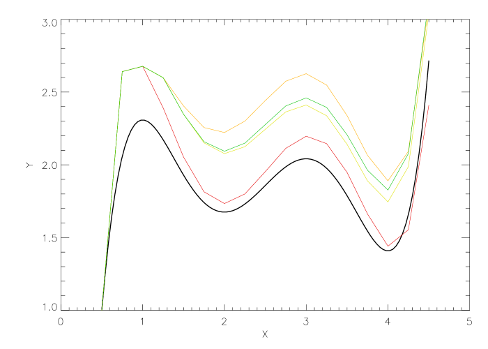
Figure 1: Adams-Bashforth solutions to polynomial test problem The analytic solution to the test problem $y^{\prime}\left(x\right)=\left(x-1\right)\left(x-2\right)\left(x-3\right)\left(x-4\right)$; $y\left(0.5\right)=1$ is plotted in bold black. Numerical solutions using a fixed grid spacing of 0.25 and AB methods of order 1 (red), 2 (orange), 3 (yellow) and 4 (green) are plotted as well. Observe that each successively higher order method deviates from the common trajectory one integration step later. This is a result of the boot-strapping technique we employ whereby the first few data points are generated by successively higher order methods until the desired order of convergence is reached. In this simple fixed-grid test case, boot-strapping produces unacceptably large errors in the first few integration steps. In production runs employing an adaptive mesh, however, the first integration step size is specified to be small enough that even a first-second order AB-AM predictor-corrector combined method produces errors smaller than the desired tolerance. Our implementation will then scale up the step size appropriately as the integration proceeds.

In Figure 2 we plot the running error accumulated by each of the AB methods previously plotted in Figure 1. Here we see that the accumulated errors of each consecutive method exhibit polynomial behavior of decreasing order, culminating in a fourth order AB method that accumulates no error greater than double-precision roundoff for our fourth-order polynomial derivative. This proves that our implementation of AB methods exhibits the expected orders of convergence.

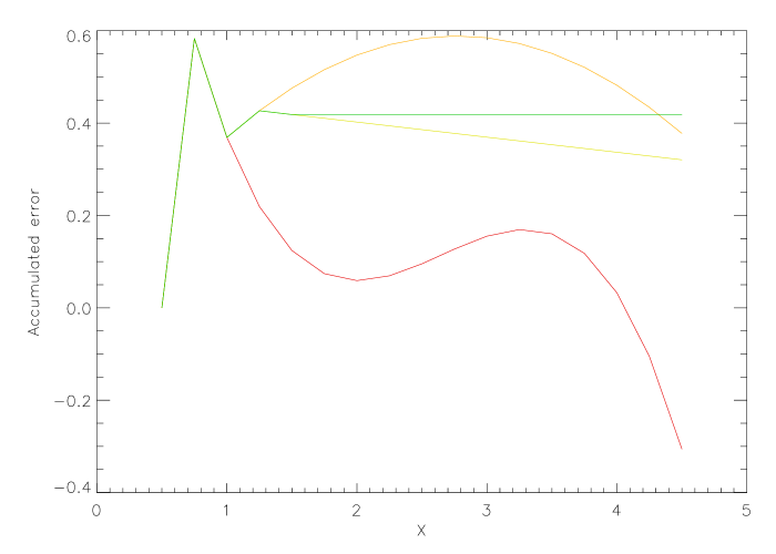
Figure 2: Accumulated error from Adams-Bashforth solutions to polynomial test problem We plot the accumulated errors with the same color convention as Figure 1. Note the polynomial behavior of the accumulated error of each method after its initial boot-strapping phase. The first order method’s error is cubic, the second order method’s error is parabolic, third order’s error is linear, and, most importantly, the fourth order AB method accumulates no error greater than roundoff. This proves that our AB methods demonstrate the expected order of convergence.

In Figure 3 we plot the solutions to our polynomial test problem achieved by ABM methods of various degrees. The fixed-grid ABM methods are plotted in the same color as the (fixed-grid) AB-only solution of the same AB order in Figure 1. For instance, the AB method of order 2 and the ABM method of order 2-3 are both plotted in orange in Figures 1 and 3, respectively. We omit the fixed-grid ABM method of order 4-5 because it is coincident with the fixed-grid ABM method of order 3-4. We also plot two adaptive-grid methods in Figure 3. The adaptive-grid ABM method of order 3-4 is plotted as a dashed curve, while the adaptive-grid ABM method of order 4-5 is plotted as a dotted curve. Even with the artificially large integration steps (or first integration step, in the adaptive-grid cases), we see that adding Adams-Moulton correction to the Adams-Bashforth prediction results in much smaller errors.

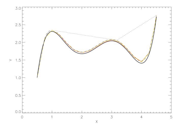
Figure 3: Adams-Bashforth-Moulton solutions to polynomial test problem We plot various solutions to our polynomial test problem. As before, the analytic solution is bold black. Fixed-grid (step size 0.25, as in Figure 1) ABM solutions are plotted in color. Each solution is plotted in the same color as the AB-only solution in Figure 1 of the same AB order. Adding the AM correction then increases the order of convergence by 1. We also plot two additional solutions on this figure. The dashed curve is the order 3-4, adaptive grid ABM method. The dotted curve is the order 4-5, adaptive grid ABM method. Note that the adaptive-grid 3-4 ABM solution must follow the curve, maintaining small step sizes. After the initial boot-strapping, the adaptive-grid 4-5 ABM method arrives at its final result in only two integration steps.

In Figure 4 we plot the error accumulated by the ABM methods discussed in Figure 3. We see that the fixed-grid methods display similar decreasing-order polynomial behavior with increasing order of convergence. As befits methods with a correction phase that increases the order of convergence by one, each curve here is a lower-by-one order polynomial compared to the curve of accumulated error of the equal AB order method’s solution (and same color) plotted in Figure 2. For instance, the red curves in 2 and 4 refer to the error accumulated by the AB method of order 1 and the ABM method of order 1-2, respectively, but the former displays cubic behavior while the latter displays parabolic. In addition, the parabolic-error curve in Figure 4 (red) deviates from the common trajectory one integration step sooner than the parabolic-error curve in Figure 2 (orange). These patterns confirm that our fixed-grid ABM methods display the expected $N$+1 order of convergence.

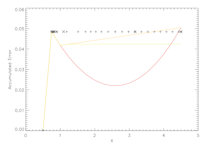
Figure 4: Accumulated error from Adams-Bashforth-Moulton solutions to Polynomial test problem We plot accumulated error for all numeric methods described in Figure 3. Colored curves denote the errors accumulated by curves of the corresponding color in that figure. For clarity, accumulated errors of the 3-4 adaptive grid ABM and 4-5 adaptive grid ABM methods are now plotted as +’s and X’s, respectively. Note that each fixed-grid ABM curve displays an order of convergence greater by one than its corresponding AB-only method, as expected. This proves that the fixed-grid ABM methods demonstrate the expected order of convergence. Also note that, for example, the method with parabolic accumulated error (ABM order 1-2) ends its bootstrapping phase one integration step earlier than the parabolic-error AB-only method (AB Order 2). This is also expected behavior for, and a benefit of, an implicit corrector.

We also plot the error accumulated by the adaptive-grid ABM methods of order 3-4 and 4-5, this time as $+$’s and $\times$’s, respectively, for clarity. We see that both have negligible accumulated error after the initial (artificially large) integration step. In this artificial problem, there are no error terms after the correction phase of the adaptive-grid ABM method of order 3-4, so we expected no error to accumulate. However, the correction phase is necessary in each integration step to capture all the behavior of the derivative, and the correction remains roughly constant in magnitude with each step. The step size thus remains roughly constant as well, because this method has no way of determining that it could increase its step size without increasing its error.

The adaptive-grid ABM method of order 4-5, in contrast, captures the entire behavior of the derivative in the AB phase, with the AM correction confirming that the errors are no larger than roundoff. After its initial boot-strapping phase, the adaptive-grid ABM method of order 4-5 can then increase its step size geometrically. Although we have no theoretical bound on how large the step size could be made, for caution in case of the coincidental vanishing of just one error term, in practice we limit its growth to geometric, with a ratio of 3. The adaptive-grid ABM method of order 4-5 arrives at its final answer in only two integration steps after its initial boot-strapping. We plot the step size for these two methods in Figure 5. The Order 3-4 and 4-5 methods are plotted as dashed and dotted, respectively, analogously to Figure 3.

Figure 5: Step size of adaptive-mesh Adams-Bashforth-Moulton solutions to polynomial test problem We plot the step sizes of the Order 3-4 and Order 4-5 ABM methods as, respectively, dashed and dotted curves, similar to Figure 3. For our fourth-order polynomial test problem, there are, in fact, no further error terms after the Order 3-4 method’s AM correction phase, but there is no way for the method to determine that. It must therefore maintain a relatively constant step size. The Order 4-5 ABM solution, in contrast, captures all information about the derivative in the AB phase already, and the AM phase confirms that there is no correction to be made. The step size is therefore increased dramatically. The divergent behavior of the two methods, with the precondition that the fixed-grid methods are known to converge as expected (See Figure 4), demonstrates that the ABM methods maintain their expected order of convergence even when the step size is allowed to change.

The errors in the initial integration step for all the methods discussed thus far have been quite large, but this is only because we have deliberately selected a very large step size parameter in order to highlight the error behavior of all these methods. In a production-quality data run using adaptive-grid ABM methods, the initial step size parameter would be selected so as to give negligible error in the first integration step, and thereafter would be rapidly increased to a size commensurate with the desired precision of integration. The step sizes decrease markedly in both of the methods shown in Figure 5 in the last integration step because the integrations have already reached the upper limit.

4 TOLMAN-OPPENHEIMER-VOLKOFF TEST PROBLEM

4.1 Motivation and Introduction

Since the ABM methods passed our polynomial test problem, we devised a more complex problem to test our implementation in a real-world setting. We selected the famous problem of deriving the maximum possible mass (as measured by an observer at infinity) of material that can be supported hydrostatically against gravitational collapse- in short, the most massive possible neutron star. Oppenheimer and Volkoff (1939) (OV) discovered the existence of this limit for any equation of state obeying relativistic causality. They also derived the numerical value of 0.71 M_⊙ for the limit under the assumption that the only contribution to pressure is that of neutron momentum arising from the Pauli exclusion principle. Their value of the radius corresponding to this mass is 9.5 km. For this problem, we expand the $y$ variable from Sections 2 and 3 into a vector whose elements are pressure and mass-energy enclosed within the radius.We discuss the details of this problem throughout the rest of this section.

4.2 Hydrostatic Equilibrium

The problem of finding the TOV limit assumes bodies in non-rotating, spherical, hydrostatic equilibrium. The Schwarzschild metric (Schwarzschild, 1916) describes this geometry:

$$\mathrm{d}s^{2}=-e^{2\Phi}\mathrm{d}t^{2}+e^{2\Lambda}\mathrm{d}r^{2}+r^{2}\mathrm{d}\Omega^{2}$$ (23)

where $s$ is the spacetime interval, $t$ is the timelike variable, $r$ is the radial spatial variable, $\Omega$ is the solid angle, and $\Phi$ and $\Lambda$ are metric functions of $r$.

From there, the equations describing non-rotating spheres in hydrostatic equilibrium can be easily derived (e.g., Misner, Thorne, and Wheeler (1973) (MTW), p. 600, their equations 23.19 and 23.22):

$$m(r)=\int_{0}^{r}4\pi\bar{r}^{2}\rho\,\mathrm{d}\bar{r}+m(0)$$ (24)

$$\frac{\mathrm{d}P}{\mathrm{d}r}=-\frac{\left(\rho+P\right)\left(m+4\pi r^{3}P\right)}{r\left(r-2m\right)}$$ (25)

where $m$ is the mass enclosed within $r$, $\rho$ is the mass-energy density expressed as an energy per volume, and $P$ is the pressure, and all of these variables are functions of $r$. Reintroducing factors of $G$ and $c$ omitted in MTW, taking the derivative with respect to $r$ in Equation 24, and explicitly stating the variable dependencies gives

$$\frac{\mathrm{d}m(r)}{\mathrm{d}r}=\frac{4\pi}{c^{2}}r^{2}\rho(r)$$ (26)

$$\frac{\mathrm{d}P(r)}{\mathrm{d}r}=-\frac{G}{c^{2}r^{2}}\left(\rho(r)+P(r)\right)\left(m(r)+\frac{4\pi}{c^{2}}r^{3}P(r)\right)\left(1-\frac{2Gm(r)}{c^{2}r}\right)^{-1}$$ (27)

These equations by themselves do not form a closed system. We discuss their closure in Section 4.3.

4.3 Equation of State

In order to form a closed system of equations, we must supplement Equations 26 and 27 with an equation of state (EOS), i.e. a relationship between $P$ and $\rho$. In order to compare to the OV results, we use the same EOS. The OV EOS assumes that pressure results only from neutrons with the minimum possible momenta allowed by the Pauli exclusion principle. Kippenhahn and Weigert, 1994 (p. 118, hereafter KW) derive an analogous relation for electrons. The identity of the particle giving rise to the pressure enters into the derivation only in the mass, so to adapt their derivation we simply replace the mass of an electron, $m_{e}$, with the mass of a neutron, $m_{n}$. Following KW, and with $n$ the number density of neutrons:

$$P(n)=\frac{\pi m_{n}^{4}c^{5}}{3h^{3}}\left(x\left(2x^{2}-3\right)\sqrt{x^{2}+1}+3\ln\left(x+\sqrt{x^{2}+1}\right)\right)$$ (28)

where

$$x\equiv\frac{h}{2m_{n}c}\sqrt[3]{\frac{3n}{\pi}}$$

The energy density has contributions both from rest mass and from the internal kinetic energy of the particles, which we shall call $U$.

$$\rho(n)=m_{n}c^{2}n+U(n)$$ (29)

We again adapt a KW expression (p. 122), this time for $U$:

$$\rho(n)=m_{n}c^{2}n+\frac{\pi m_{n}^{4}c^{5}}{3h^{3}}\left(3x\left(2x^{2}+1\right)\sqrt{x^{2}+1}-8x^{3}-3\ln\left(x+\sqrt{x^{2}+1}\right)\right)$$ (30)

We will need to solve Equations 28 and 30 numerically to eliminate $n$.

4.4 A Single Integration

We use an ABM method to integrate Equations 26 and 27 over $r$, supplemented by Equations 28 and 30, in the following manner. We select a value for central pressure. This single boundary condition spans the solution space for our system of equations. We then invert Equation 28 numerically in order to determine the number density of neutrons $n$. The number density is inserted into Equation 30 to find $\rho$. Since we have selected an EOS intended for use in neutron stars, we select an initial integration step size, that is, $\Delta r_{0}$, so small as to give negligible errors even in the first integration step, which given our bootstrapping technique will be an order 1-2 ABM method. We have determined that 10 cm is quite sufficiently small. We then have enough information to determine the derivatives of both quantities to be integrated, $m(r)$ and $P(r)$, via Equations 26 and 27. We update the $\Delta r$ using the predictor-corrector technique. The integration gives us the next value of $P(r)$, so we can repeat this procedure, increasing the order of the ABM method by one each step until the maximum desired order is reached. We halt the integration when $P(r)$ reaches or overshoots zero. The total mass and radius of the hydrostatic sphere, $M$ and $R$, respectively, are defined as the final values of $m(r)$ and $r$.

4.5 Parameter Hunts

Some experimentation with different central pressures in the procedure outlined in Section 4.4 will quickly reveal that the neutron star corresponding to the TOV limit in this EOS must have a central pressure that lies between 10${}^{\text{35}}$ and 10${}^{\text{36}}$ erg cm${}^{\text{-3}}$. We use a trinary sieve to reduce that range to 3.631382 x 10${}^{\text{35}}$ erg cm${}^{\text{-3}}$ $\pm$ 16 in the final two decimal places. During the sieving, we use an initial step size of 10 cm, an ABM method of order 6-7, and a desired stepwise tolerance of 10${}^{\text{-8}}$. To ensure that the each integration will terminate in a reasonable period of time even in the face of the dramatic vanishing of pressure near the surface, we force the step size to remain at least 10 cm. The midpoint of our pressure range, with the same integration parameters except an ABM order of 10-11, gives a total mass of 0.71017188 M_⊙ and a radius of 9.16233 km. Oppenheimer and Volkoff (1939) arrived at values of 0.71 M_⊙ and 9.5 km. We have achieved perfect agreement in total mass within the precision of their published results, but we do have a discrepancy of some 300 m or roughly 3.5% in radius. OV do not disclose their method of numerical integration, but we believe it is certainly plausible that a pre-WWII numerical integration would have a precision of worse than 3.5% in the independent variable. This is especially true when its precise value was then of so little interest compared to the mass, and when the final radius has so little bearing on the former: the density in the last few percent of radius is less by many orders of magnitude than the central density, so the thickness of the crust is negligible with respect to the total mass.

With superhigh-precision estimates in hand for the mass and radius, we then conduct a parameter sweep in the tolerance and order of convergence for what combinations produce the best combination of agreement with the superhigh-precision results and few steps necessary to complete the integration. We have compiled our results in Table 1.

Table 1: Integration Steps Required for Different Parameters, and the Precision of Corresponding Data We tabulate the integration steps required to arrive at a full solution for various ABM adaptive-grid methods (listed in the table by AB-phase order only) and for various target step-wise maximum fractional AM corrections. The number listed in the large table at left is the number of integration steps. The precision with which a given set of parameters will match the total mass as calculated by the superhigh-precision method in the lower right corner is indicated by the color in which the integration step is written. For instance, parameter sets that deliver solutions with total neutron star mass matching the superhigh-precision parameters within 1% are written in dark blue. The precision with which a parameter set matches the superhigh-precision radius are shown as colored contours. For instance, parameter sets delivering a radius within one part in 1000 of the superhigh-precision radius are inside the yellow contour. For maximal agreement with the superhigh-precision solution in total M and total R, we find that an ABM order of 9-10 coupled with a desired stepwise correction tolerance of 10${}^{\text{-5}}$ arrives at a solution in only 131 steps, while we can achieve a 1% solution in 27 steps with an ABM order of 4-5 coupled with a stepwise correction tolerance of 10${}^{\text{-2}}$. These two parameter sets are explored in more detail throughout this section.

We list the number of steps required for each combination of parameters to terminate in Table 1 and higlight the precision of agreement with the high-precision results for mass and radius using colors. The color of the font denotes the precision of agreement with the mass value of 0.71017188 M_⊙. Contour lines denote the precision of agreement with the radius value of 9.16233 km. We find that two parameter combinations are especially efficient for their desired precision. A tolerance of 10${}^{\text{-2}}$ and an ABM order of 4-5 achieves 1% precision in both mass and radius in only 27 integration steps. A tolerance of 10${}^{\text{-5}}$ and an ABM order of 9-10 achieves maximal precision in mass and radius (10${}^{\text{-8}}$ and 10${}^{\text{-5}}$, respectively) in 131 integration steps. We will refer to these combinations as the low precision and high precision solutions, respectively, henceforth. The remainder of this section is devoted to investigating these specific combinations in greater detail.

In Figure 6 we plot the step sizes of each of our highlighted solutions. We limit the step size to increase by at most a factor of 3 in each step, in order not to miss any sudden changes in behavior that might appear. Both curves follow this upper bound for several steps, indicating that our choice of initial step size was small enough not to accumulate any significant error during bootstrapping. The step size then plateaus for the bulk of the radius and then shrinks near the surface, where much greater resolution is needed.

Figure 6: Step size for high (solid) and low (dashed) precision ABM solutions to the Tolman-Oppenheimer-Volkoff test problem We see that both solutions exhibit initial exponential growth of step size. For caution, we allow the step size to increase geometrically at each integration step with only a maximum ratio of 3. Both curves maintain that maximal growth for several integration steps, indicating that our choice of initial step size was small enough that any error accumulated during the bootstrapping phase should be well below the specified desired precision for each curve. The plateau through the bulk of each integration is followed by dramatic declines as much greater resolution is needed near the surface of the sphere.

In Figure 7 we demonstrate that, after bootstrapping, the AM correction term remains quite stable throughout most of the integration steps, increasing only in the final few.

Figure 7: AM fractional correction term for high (solid) and low (dashed) precision ABM solutions to the Tolman-Oppenheimer-Volkoff test problem Here we see that both curves maintain stable precision at the desired level for integration.

In Figure 8 we discover the reason for the increasing size of correction term as shown in Figure 7. We overplot the log of pressure in arbitrary units (bold black curve) as a function of radius. This shows that the dramatic dropoff in pressure near the surface is the controlling factor in the need for greater resolution.

Figure 8: Step size vs. r for high (solid) and low (dashed) precision ABM solutions to the Tolman-Oppenheimer-Volkoff test problem In order to clarify why the step size decreases the way it does, we overplot the log of pressure (in arbitrary units) in a solid, bold line. It is the dramatic behavior of the pressure near the surface that accounts for the largest error correction terms, and therefore the decreasing step size.

5 CONCLUSIONS

We have demonstrated that our integration methods exhibit the expected order of convergence with various levels of sophistication activated:

1. Adams-Bashforth-only, fixed-grid, explicit methods

2. Adams-Bashforth-Moulton, fixed-grid, explicit-implicit, predictor-corrector methods

3. Adams-Bashforth-Moulton, adaptive-grid, explicit-implicit, predictor-corrector methods.

Furthermore, we have shown that our methods can arrive at high-quality, robust solutions to real-world research questions in a very small number of integration steps that require fewer derivative evaluations than more favored method families.

6 ACKNOWLEDGEMENTS

This research was made possible in part by a grant from the Maine Space Grant Consortium, two Frank H. Todd scholarships, and a Summer Graduate Research Fellowship and University Graduate Research Assistantship from the University of Maine. The author would like to thank Chris Fryer and Kent Budge of Los Alamos National Laboratory for encouragement to pursue this line of research, Neil F. Comins of the University of Maine for helpful discussions and editing of this paper, and my wife Kate and daughter Evangeline for my entire universe.

References

- Bashforth and Adams (1883) Bashforth, F. & Adams, J. C. 1883, An Attempt to test the Theories of Capillary Action by comparing the theoretical and measured forms of drops of fluid. With an explanation of the method of integration employed in constructing the tables which give the theoretical forms of such drops, (Cambridge University Press)
- Courant, Friedrichs, and Lewy (1928) Courant, R., Friedrichs, K., & Lewy, H. 1928, Mathematische Annalen, 100, 1, pp. 32–74
- Kippenhahn and Weigert (1994) Kippenhahn, R., & Weigert, A. 1994, Stellar Structure and Evolution (Springer)
- Misner, Thorne, and Wheeler (1973) Misner, C., Thorne, K., & Wheeler, J. 1973, Gravitation (1973, W.H. Freeman and Company)
- Moulton (1926) Moulton, F. R. 1926, New Methods in Exterior Ballistics (University of Chicago Press)
- Oppenheimer and Volkoff (1939) Oppenheimer, J. R. & Volkoff, G. M. 1939, Phys. Rev., 55-4, pp. 374–381
- Runge (1895) Runge, C. 1895, Math. Ann. 46, pp. 167–178
- Runge (1901) Runge, C. 1901, Zeitschrift f r Mathematik und Physik 46: 224–243
- Schwarzschild (1916) Schwarzschild, K. 1916, Proc. Royal Prussian Acad. Sci. meeting on 3 February 1916, p. 189-196
- Tolman (1934) Tolman, R. C. 1934, Proc. Nat. Acad. Sci. 20 (3): 169–176