‘Standard’ Cosmological model & beyond with CMB

Abstract

Observational Cosmology has indeed made very rapid progress in the past decade. The ability to quantify the universe has largely improved due to observational constraints coming from structure formation Measurements of CMB anisotropy and, more recently, polarization have played a very important role. Besides precise determination of various parameters of the ‘standard’ cosmological model, observations have also established some important basic tenets that underlie models of cosmology and structure formation in the universe – ‘acausally’ correlated initial perturbations in a flat, statistically isotropic universe, adiabatic nature of primordial density perturbations. These are consistent with the expectation of the paradigm of inflation and the generic prediction of the simplest realization of inflationary scenario in the early universe. Further, gravitational instability is the established mechanism for structure formation from these initial perturbations. The signature of primordial perturbations observed as the CMB anisotropy and polarization is the most compelling evidence for new, possibly fundamental, physics in the early universe. The community is now looking beyond the estimation of parameters of a working ‘standard’ model of cosmology for subtle, characteristic signatures from early universe physics.

1 Introduction

The ‘standard’ model of cosmology must not only explain the dynamics of the homogeneous background universe, but also satisfactorily describe the perturbed universe – the generation, evolution and finally, the formation of large scale structures in the universe. It is fair to say much of the recent progress in cosmology has come from the interplay between refinement of the theories of structure formation and the improvement of the observations.

The transition to precision cosmology has been spearheaded by measurements of CMB anisotropy and, more recently, polarization. Despite its remarkable success, the ‘standard’ model of cosmology remains largely tied to a number of fundamental assumptions that have yet to find complete and precise observational verification : the Cosmological Principle, the paradigm of inflation in the early universe and its observable consequences (flat spatial geometry, scale invariant spectrum of primordial seed perturbations, cosmic gravitational radiation background etc.). Our understanding of cosmology and structure formation necessarily depends on the rather inaccessible physics of the early universe that provides the stage for scenarios of inflation (or related alternatives). The CMB anisotropy and polarization contains information about the hypothesized nature of random primordial/initial metric perturbations – (Gaussian) statistics, (nearly scale invariant) power spectrum, (largely) adiabatic vs. iso-curvature and (largely) scalar vs. tensor component. The ‘default’ settings in brackets are motivated by inflation. The signature of primordial perturbations on super-horizon scales at decoupling in the CMB anisotropy and polarization are the most definite evidence for new physics (eg., inflation ) in the early universe that needs to be uncovered. However, the precision estimation of cosmological parameters implicitly depend on the assumed form of the initial conditions such as the primordial power spectrum, or, explicitly on the scenario of generation of initial perturbations [1, 2].

Besides precise determination of various parameters of the ‘standard’ cosmological model, observations have also begum to establish (or observationally query) some of the important basic tenets of cosmology and structure formation in the universe – ‘acausally’ correlated initial perturbations, adiabatic nature of primordial density perturbations, gravitational instability as the mechanism for structure formation. We have inferred a spatially flat universe where structures form by the gravitational evolution of nearly scale invariant, adiabatic perturbations in the non–baryonic cold dark matter. There is a dominant component of dark energy that does not cluster (on astrophysical scales). We briefly review the observables from the CMB sky and importance to understanding cosmology in section 2 Most recent estimates of the cosmological parameters are available and best obtained from recent literature, eg. Ref.[3] and, hence, is not given in the article. The main theme of the article is to highlight the success of recent cosmological observations in establishing some of the fundamental tenets of cosmology and structure :

• Statistical Isotropy of the universe (Sec. 3);

• Gravitational instability mechanism for structure formation(Sec. 4);

• Primordial perturbations from Inflation.(Sec. 5).

Up to this time, the attention of the community has been largely focused on estimating the cosmological parameters. The next decade would see increasing efforts to observationally test fundamental tenets of the cosmological model and search for subtle deviations from the same using the CMB anisotropy and polarization measurements and related LSS observations, galaxy survey, gravitational lensing, etc.

2 CMB observations and cosmological parameters

The angular power spectra of the Cosmic Microwave Background temperature fluctuations ($C_{\ell}$)have become invaluable observables for constraining cosmological models. The position and amplitude of the peaks and dips of the $C_{\ell}$ are sensitive to important cosmological parameters, such as, the relative density of matter, $\Omega_{0}$; cosmological constant, $\Omega_{\Lambda}$; baryon content, $\Omega_{B}$; Hubble constant, $H_{0}$ and deviation from flatness (curvature), $\Omega_{K}$.

The angular spectrum of CMB temperature fluctuations has been measured with high precision on up to angular scales ($\ell\sim 1000$) by the WMAP experiment [3], while smaller angular scales have been probed by ground and balloon-based CMB experiments such as ACBAR, QuaD and ACT [4, 5]. These data are largely consistent with a $\Lambda$CDM model in which the Universe is spatially flat and is composed of radiation, baryons, neutrinos and, the exotic, cold dark matter and dark energy. The exquisite measurements by the Wilkinson Microwave Anisotropy Probe (WMAP) mark a successful decade of exciting CMB anisotropy measurements and are considered a milestone because they combine high angular resolution with full sky coverage and extremely stable ambient condition (that control systematics) allowed by a space mission . Figure 1 shows the angular power spectrum of CMB temperature fluctuations obtained from the 5 & 7-year WMAP data [6].

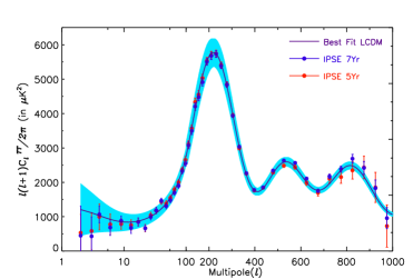
Figure 1: The angular power spectrum estimated from the multi-frequency five and seven year WMAP data. The result from IPSE a self-contained model free approach to foreground removal  [6] matches that obtained by the WMAP team. The solid curve showing prediction of the best fit power-law, flat, $\Lambda$CDM model threads the data points closely.[Fig. courtesy: Tuhin Ghosh]

The measurements of the anisotropy in the cosmic microwave background (CMB) over the past decade has led to ‘precision cosmology’. Observations of the large scale structure in the distribution of galaxies, high redshift supernova, and more recently, CMB polarization, have provided the required complementary information. The current up to date status of cosmological parameter estimates from joint analysis of CMB anisotropy and Large scale structure (LSS) data is usually best to look up in the parameter estimation paper accompanying the most recent results announcement of a major experiment, such as recent WMAP release [3].

One of the firm predictions of this working ‘standard’ cosmological model is linear polarization pattern ($Q$ and $U$ Stokes parameters) imprinted on the CMB at last scattering surface. Thomson scattering generates CMB polarization anisotropy at decoupling [8]. This arises from the polarization dependence of the differential cross section: $d\sigma/d\Omega\propto|\epsilon^{\prime}\cdot\epsilon|^{2}$, where $\epsilon$ and $\epsilon^{\prime}$ are the incoming and outgoing polarization states [9] involving linear polarization only. A local quadrupole temperature anisotropy produces a net polarization, because of the $\cos^{2}\theta$ dependence of the cross section. A net pattern of linear polarization is retained due to local quadrupole intensity anisotropy of the CMB radiation impinging on the electrons at $z_{rec}$. The polarization pattern on the sky can be decomposed in the two kinds with different parities. The even parity pattern arises as the gradient of a scalar field called the $E$–mode. The odd parity pattern arises from the ‘curl’ of a pseudo-scalar field called the $B$–mode of polarization. Hence the CMB sky maps are characterized by a triplet of random scalar fields: $X(\hat{n})\equiv\{T(\hat{n})$, $E(\hat{n})$, $B(\hat{n})\}$. For Gaussian CMB sky, there are a total of 4 power spectra that characterize the CMB signal : $C^{\rm TT}_{\ell},C^{\rm TE}_{\ell},C^{\rm EE}_{\ell},C^{\rm BB}_{\ell}$. Parity conservation eliminates the two other possible power spectra, $C^{\rm TB}_{\ell}$ & $C^{\rm EB}_{\ell}$. While CMB temperature anisotropy can also be generated during the propagation of the radiation from the last scattering surface, the CMB polarization signal can be generated primarily at the last scattering surface, where the optical depth transits from large to small values. The polarization information complements the CMB temperature anisotropy by isolating the effect at the last scattering surface from effects along the line of sight.

The CMB polarization is an even cleaner probe of early universe scenarios that promises to complement the remarkable successes of CMB anisotropy measurements. The CMB polarization signal is much smaller than the anisotropy signal. Measurements of polarization at sensitivities of $\mu K$ (E-mode) to tens of $nK$ level (B-mode) pose stiff challenges for ongoing and future experiments.

After the first detection of CMB polarization spectrum by the Degree Angular Scale Interferometer (DASI) on the intermediate band of angular scales ($l\sim 200-440$) in late 2002 [10], the field has rapidly grown, with measurements coming in from a host of ground–based and balloon–borne dedicated CMB polarization experiments. The full sky E-mode polarization maps and polarization spectra from WMAP were a new milestone in CMB research [11, 12]. The most current CMB polarization measurement of $C^{\rm TT}_{\ell}$, $C^{\rm TE}_{\ell}$ and $C^{\rm EE}_{\ell}$ and a non–detection of $B$–modes come from QUaD and BICEP. They also report interesting upper limits $C^{\rm TB}_{\ell}$ or $C^{\rm EB}_{\ell}$, over and above observational artifacts [13]. A non-zero detection of $C^{\rm TB}_{\ell}$ or $C^{\rm EB}_{\ell}$, over and above observational artifacts, could be tell-tale signatures of exotic parity violating physics [14] and the CMB measurements put interesting limits on these possibilities.

While there has been no detection of cosmological signal in B-mode of polarization, the lack of $B$–mode power suggests that foreground contamination is at a manageable level which is good news for future measurements. The Planck satellite launched in May 2009 will greatly advance our knowledge of CMB polarization by providing foreground/cosmic variance–limited measurements of $C^{\rm TE}_{\ell}$ and $C^{\rm EE}_{\ell}$ out beyond $l\sim 1000$. We also expect to detect the weak lensing signal, although with relatively low precision. Perhaps, Planck could detect inflationary gravitational waves if they exist at a level of $r\sim 0.1$. In the future, a dedicated CMB polarization mission is under study at both NASA and ESA in the time frame 2020+. These primarily target the $B$-mode polarization signature of gravity waves, and consequently, identify the viable sectors in the space of inflationary parameters.

3 Statistical Isotropy of the universe

The Cosmological Principle that led to the idealized FRW universe found its strongest support in the discovery of the (nearly) isotropic, Planckian, Cosmic Microwave Background. The isotropy around every observer leads to spatially homogeneous cosmological models. The large scale structure in the distribution of matter in the universe (LSS) implies that the symmetries incorporated in FRW cosmological models ought to be interpreted statistically.

The CMB anisotropy and its polarization is currently the most promising observational probe of the global spatial structure of the universe on length scales close to, and even somewhat beyond, the ‘horizon’ scale ($\sim cH_{0}^{-1}$). The exquisite measurement of the temperature fluctuations in the CMB provide an excellent test bed for establishing the statistical isotropy (SI) and homogeneity of the universe. In ‘standard’ cosmology, CMB anisotropy signal is expected to be statistically isotropic, i.e., statistical expectation values of the temperature fluctuations $\Delta T(\hat{q})$ are preserved under rotations of the sky. In particular, the angular correlation function $C(\hat{q},\,\hat{q}^{\prime})\equiv\langle\Delta T(\hat{q})\Delta T(\hat{q}^{\prime})\rangle$ is rotationally invariant for Gaussian fields. In spherical harmonic space, where $\Delta T(\hat{q})=\sum_{lm}a_{lm}Y_{lm}(\hat{q})$, the condition of statistical isotropy (SI) translates to a diagonal $\langle a_{lm}a^{*}_{l^{\prime}m^{\prime}}\rangle=C_{l}\delta_{ll^{\prime}}\delta_{mm^{\prime}}$ where $C_{l}$, is the widely used angular power spectrum of CMB anisotropy. The $C_{l}$ is a complete description only of (Gaussian) SI CMB sky CMB anisotropy and would be (in principle) an inadequate measure for comparing models when SI is violated [15].

Interestingly enough, the statistical isotropy of CMB has come under a lot of scrutiny after the WMAP results. Tantalizing evidence of SI breakdown (albeit, in very different guises) has mounted in the WMAP first year sky maps, using a variety of different statistics. It was pointed out that the suppression of power in the quadrupole and octopole are aligned [16]. Further “multipole-vector” directions associated with these multipoles (and some other low multipoles as well) appear to be anomalously correlated [17, 18]. There are indications of asymmetry in the power spectrum at low multipoles in opposite hemispheres [19]. Analysis of the distribution of extrema in WMAP sky maps has indicated non-Gaussianity, and to some extent, violation of SI [20]. The more recent WMAP maps are consistent with the first-year maps up to a small quadrupole difference. The additional years of data and the improvements in analysis has not significantly altered the low multipole structures in the maps [21]. Hence, ‘anomalies’ persisted at the same modest level of significance and are unlikely to be artifacts of noise, systematics, or the analysis in the first year data. The cosmic significance of these ‘anomalies’ remains debatable also because of the aposteriori statistics employed to ferret them out of the data. The WMAP team has devoted an entire publication to discuss and present a detailed analysis of the various anomalies [22].

The observed CMB sky is a single realization of the underlying correlation, hence detection of SI violation, or correlation patterns, pose a great observational challenge. It is essential to develop a well defined, mathematical language to quantify SI and the ability to ascribe statistical significance to the anomalies unambiguously. The Bipolar spherical harmonic (BipoSH) representation of CMB correlations has proved to be a promising avenue to characterize and quantify violation of statistical isotropy.

Two point correlations of CMB anisotropy, $C(\hat{n}_{1},\,\hat{n}_{2})$, are functions on $S^{2}\times S^{2}$, and hence can be generally expanded as

$$C(\hat{n}_{1},\,\hat{n}_{2})\,=\,\sum_{l_{1},l_{2},\ell,M}A^{\ell M}_{l_{1}l_{2}}Y^{l_{1}l_{2}}_{\ell M}(\hat{n}_{1},\,\hat{n}_{2})\,.$$ (1)

Here $A^{\ell M}_{l_{1}l_{2}}$ are the Bipolar Spherical harmonic (BipoSH) coefficients of the expansion and $Y^{l_{1}l_{2}}_{\ell M}(\hat{n}_{1},\,\hat{n}_{2})$ are bipolar spherical harmonics. Bipolar spherical harmonics form an orthonormal basis on $S^{2}\times S^{2}$ and transform in the same manner as the spherical harmonic function with $\ell,\,M$ with respect to rotations. Consequently, inverse-transform of $C(\hat{n}_{1},\,\hat{n}_{2})$ in eq. (1) to obtain the BipoSH coefficients of expansion is unambiguous.

Most importantly, the Bipolar Spherical Harmonic (BipoSH) coefficients, $A^{\ell M}_{l_{1}l_{2}}$, are linear combinations of off-diagonal elements of the harmonic space covariance matrix,

$$A^{\ell M}_{l_{1}l_{2}}\,=\,\sum_{m_{1}m_{2}}\langle a_{l_{1}m_{1}}a^{*}_{l_{2}m_{2}}\rangle(-1)^{m_{2}}{\mathcal{C}}^{\ell M}_{l_{1}m_{1}l_{2}-m_{2}}$$ (2)

where ${\mathcal{C}}_{l_{1}m_{1}l_{2}m_{2}}^{\ell M}$ are Clebsch-Gordan coefficients and completely represent the information of the covariance matrix.

Statistical isotropy implies that the covariance matrix is diagonal, $\langle a_{lm}a^{*}_{l^{\prime}m^{\prime}}\rangle=C_{l}\,\,\delta_{ll^{\prime}}\delta_{mm^{\prime}}$ and hence the angular power spectra carry all information of the field. When statistical isotropy holds BipoSH coefficients, $A^{\ell M}_{ll^{\prime}}$, are zero except those with $\ell=0,M=0$ which are equal to the angular power spectra up to a $(-1)^{l}(2l+1)^{1/2}$ factor. Therefore to test a CMB map for statistical isotropy, one should compute the BipoSH coefficients for the maps and look for nonzero BipoSH coefficients. Statistically significant deviations of BipoSH coefficient of map from zero would establish violation of statistical isotropy.

Since $A^{\ell M}_{l_{1}l_{2}}$ form an equivalent representation of a general two point correlation function, cosmic variance precludes measurement of every individual $A^{\ell M}_{l_{1}l_{2}}$. There are several ways of combining BipoSH coefficients into different observable quantities that serve to highlight different aspects of SI violations. Among the several possible combinations of BipoSH coefficients, the Bipolar Power Spectrum (BiPS) has proved to be a useful tool with interesting features [23]. BiPS of CMB anisotropy is defined as a convenient contraction of the BipoSH coefficients

$$\kappa_{\ell}\,=\,\sum_{l,l^{\prime},M}W_{l}W_{l^{\prime}}\left|A^{\ell M}_{ll^{\prime}}\right|^{2}\geq 0$$ (3)

where $W_{l}$ is the window function that corresponds to smoothing the map in real space by symmetric kernel to target specific regions of the multipole space and isolate the SI violation on corresponding angular scales.

The BipoSH coefficients can be summed over $l$ and $l^{\prime}$ to reduce the cosmic variance, to as obtain reduced BipoSH (rBipoSH) coefficients [24]

$$A_{\ell M}=\sum_{l=0}^{\infty}\sum_{l^{\prime}=|\ell-l|}^{\ell+l}A^{\ell M}_{ll^{\prime}}.$$ (4)

Reduced bipolar coefficients orientation information of the correlation patterns. An interesting way of visualizing these coefficients is to make a Bipolar map from $A_{\ell M}$

$$\Theta(\hat{n})=\sum_{\ell=0}^{\infty}\sum_{M=-\ell}^{\ell}A_{\ell M}Y_{\ell M}(\hat{n}).$$ (5)

The symmetry $A_{\ell M}=(-1)^{M}A_{\ell-M}^{*}$ of reduced bipolar coefficients guarantees reality of $\Theta(\hat{n})$.

It is also possible to obtain a measurable band power measure of $A^{\ell M}_{l_{1}l_{2}}$ coefficient by averaging $l_{1}$ in bands in multipole space. Recently, the WMAP team has chosen to quantify SI violation in the CMB anisotropy maps by the estimation $A^{\ell M}_{ll-i}$ for small value of bipolar multipole, $L$, band averaged in multipole $l$. Fig. 2 taken from the WMAP-7 release paper [22] shows SI violation measured in WMAP CMB maps

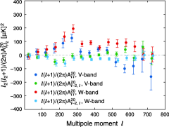
Figure 2: Figure taken from WMAP-7 yr publication on anomalies in the CMB sky [22] shows the measured quadrupolar (bipolar index $L=2$) bipolar power spectra for V-band and W-band WMAP data, using the KQ75y7 mask. The spherical multipole have been binned within uniform bands $\delta l=50$. Only the components of the bipolar power spectra with M = 0 in ecliptic coordinates are shown. A statistically significant quadrupolar effect is seen, even for a single frequency band in a single angular bin.

CMB polarization maps over large areas of the sky have been recently delivered by experiments in the near future. The statistical isotropy of the CMB polarization maps will be an independent probe of the cosmological principle. Since CMB polarization is generated at the surface of last scattering, violations of statistical isotropy are pristine cosmic signatures and more difficult to attribute to the local universe. The Bipolar Power spectrum has been defined and implemented for CMB polarization and show great promise [25].

4 Gravitational instability mechanism for structure formation

It is a well accepted notion that the large scale structure in the distribution of matter in the present universe arose due to gravitational instability from the same primordial perturbation seen in the CMB anisotropy at the epoch of recombination. This fundamental assumption in our understanding of structure formation has recently found a strong direct observational evidence [26, 27].

The acoustic peaks occur because the cosmological perturbations excite acoustic waves in the relativistic plasma of the early universe [28, 29, 30, 31, 32]. The recombination of baryons at redshift $z\approx 1100$ effectively decouples the baryon and photons in the plasma abruptly switching off the wave propagation. In the time between the excitation of the perturbations and the epoch of recombination, modes of different wavelength can complete different numbers of oscillation periods. This translates the characteristic time into a characteristic length scale and produces a harmonic series of maxima and minima in the CMB anisotropy power spectrum. The acoustic oscillations have a characteristic scale known as the sound horizon, which is the comoving distance that a sound wave could have traveled up to the epoch of recombination. This physical scale is determined by the expansion history of the early universe and the baryon density that determines the speed of acoustic waves in the baryon-photon plasma.

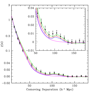
Figure 3: The large-scale redshift-space correlation function of the SDSS LRG sample taken from Ref. [26]. The inset shows an expanded view with a linear vertical axis. The lower-most curve (magenta), which lacks the acoustic peak, shows a pure CDM model ($\Omega_{m}h^{2}=0.105$). The models are $\Omega_{m}h^{2}=0.12$ (top-most, green), 0.13 (red), and 0.14 (bottom-most with peak, blue), all with $\Omega_{b}h^{2}=0.024$ and $n=0.98$ and with a mild non-linear prescription folded in. The clearly visible bump at $\sim 100h^{-1}{\rm\,Mpc}$ scale is statistically significant.

For baryonic density comparable to that expected from Big Bang nucleosynthesis, acoustic oscillations in the baryon-photon plasma will also be observably imprinted onto the late-time power spectrum of the non-relativistic matter. This is easier understood in a real space description of the response of the CDM and baryon-photon fluid to metric perturbations [26]. An initial small delta-function (sharp spike) adiabatic perturbation ($\delta\ln a|_{H}$) at a point leads to corresponding spikes in the distribution of cold dark matter (CDM), neutrinos, baryons and radiation (in the ‘adiabatic’ proportion, $1+w_{i}$, of the species). The CDM perturbation grows in place while the baryonic perturbation being strongly coupled to radiation is carried outward in an expanding spherical wave. At recombination, this shell is roughly $105h^{-1}{\rm\,Mpc}$ in (comoving) radius when the propagation of baryons ceases. Afterward, the combined dark matter and baryon perturbation seeds the formation of large-scale structure. The remnants of the acoustic feature in the matter correlations are weak ($10\%$ contrast in the power spectrum) and on large scales. The acoustic oscillations of characteristic wave-number translates to a bump (a spike softened by gravitational clustering of baryon into the well developed dark matter over-densities) in the correlation function at $105h^{-1}{\rm\,Mpc}$ separation. The large-scale correlation function of a large spectroscopic sample of luminous, red galaxies (LRGs) from the Sloan Digital Sky Survey that covers $\sim 4000$ square degrees out to a redshift of $z\sim 0.5$ with $\sim 50,000$ galaxies has allowed a clean detection of the acoustic bump in distribution of matter in the present universe. Figure 3 shows the correlation function derived from SDSS data that clearly shows the acoustic ‘bump’ feature at a fairly good statistical significance [26]. The acoustic signatures in the large-scale clustering of galaxies provide direct, irrefutable evidence for the theory of gravitational clustering, notably the idea that large-scale fluctuations grow by linear perturbation theory from $z\sim 1000$ to the present due to gravitational instability.

5 Primordial perturbations from Inflation

Any observational comparison based on structure formation in the universe necessarily depends on the assumed initial conditions describing the primordial seed perturbations. It is well appreciated that in ‘classical’ big bang model the initial perturbations would have had to be generated ‘acausally’. Besides resolving a number of other problems of classical Big Bang, inflation provides a mechanism for generating these apparently ‘acausally’ correlated primordial perturbations [33].

The power in the CMB temperature anisotropy at low multipoles ($l\mathrel{\hbox to0.0pt{\lower 4.0pt\hbox{\hskip 1.0pt$\sim$}\hss}\raise 1.0pt\hbox{$<$}}60$) first measured by the COBE-DMR [34] did indicate the existence of correlated cosmological perturbations on super Hubble-radius scales at the epoch of last scattering, except for the (rather unlikely) possibility of all the power arising from the integrated Sachs-Wolfe effect along the line of sight. Since the polarization anisotropy is generated only at the last scattering surface, the negative trough in the $C_{l}^{TE}$ spectrum at $l\sim 130$ (that corresponds to a scale larger than the horizon at the epoch of last scattering) measured by WMAP first sealed this loophole, and provides an unambiguous proof of apparently ‘acausal’ correlations in the cosmological perturbations [11, 12, 35].

Besides, the entirely theoretical motivation of the paradigm of inflation, the assumption of Gaussian, random adiabatic scalar perturbations with a nearly scale invariant power spectrum is arguably also the simplest possible choice for the initial perturbations. What has been truly remarkable is the extent to which recent cosmological observations have been consistent with and, in certain cases, even vindicated the simplest set of assumptions for the initial conditions for the (perturbed) universe discussed below.

5.1 Nearly zero curvature of space

The most interesting and robust constraint obtained in our quests in the CMB sky is that on the spatial curvature of the universe. The combination of CMB anisotropy, LSS and other observations can pin down the universe to be flat, $\Omega_{K}\approx-0.02\pm 0.02$. This is based on the basic geometrical fact that angular scale subtended in the sky by the acoustic horizon would be different in a universe with uniform positive (spherical), negative (hyperbolic), or, zero (Euclidean) spatial curvature. Inflation dilutes the curvature of the universe to negligible values and generically predicts a (nearly) Euclidean spatial section.

5.2 Adiabatic primordial perturbation

The polarization measurements provides an important test on the adiabatic nature primordial scalar fluctuations . CMB polarization is sourced by the anisotropy of the CMB at recombination, $z_{rec}$, the angular power spectra of temperature and polarization are closely linked. Peaks in the polarization spectra are sourced by the velocity term in the same acoustic oscillations of the baryon-photon fluid at last scattering. Hence, a clear indication of the adiabatic initial conditions is the compression and rarefaction peaks in the temperature anisotropy spectrum be ‘out of phase’ with the gradient (velocity) driven peaks in the polarization spectra.

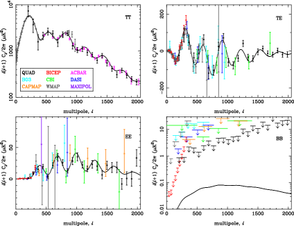
Figure 4: Figure taken from Ref. [4] show a compilation of recent measurements of the angular power spectra CMB anisotropy and polarization from a number of CMB experiments. The data is good enough to indicate that the peaks in EE and TE are out of phase with that of TT as expected for adiabatic initial conditions. The null BB detection of primary CMB signal from gravity waves is not unexpected (given the ratio of tensor to scalar perturbations).

The figure 4 taken from Ref. [4] reflects the current observational status of CMB E-mode polarization measurements. The recent measurements of the angular power spectrum the E-mode of CMB polarization at large $l$ have confirmed that the peaks in the spectra are out of phase with that of the temperature anisotropy spectrum.

5.3 Nearly scale-invariant power spectrum ?

In a simple power law parametrization of the primordial spectrum of density perturbation ($|\delta_{k}|^{2}=Ak^{n_{s}}$), the scale invariant spectrum corresponds to $n_{s}=1$. Estimation of (smooth) deviations from scale invariance favor a nearly scale invariant spectrum [3]. Current observations favor a value very close to unity are consistent with a nearly scale invariant power spectrum.

Figure 5: The primordial power spectrum recovered from the angular power spectrum of CMB anisotropy measured by WMAP for a concordance cosmological model is shown as the solid curve. Strongest deviation from a scale invariant Harrison-Zeldovich spectrum (which here will be a flat line) is the sharp infra-red cut-off at the horizon scale. The dotted lines correspond to the recovered spectra when cosmological parameters are varied within their $1-\sigma$ error bars and demonstrate the robustness of features in the recovered spectrum.

While the simplest inflationary models predict that the spectral index varies slowly with scale, inflationary models can produce strong scale dependent fluctuations. Many model-independent searches have also been made to look for features in the CMB power spectrum [37, 38, 39, 40]. Accurate measurements of the angular power spectrum over a wide range of multipoles from the WMAP has opened up the possibility to deconvolve the primordial power spectrum for a given set of cosmological parameters [41, 42, 43, 44]. The primordial power spectrum has been deconvolved from the angular power spectrum of CMB anisotropy measured by WMAP using an improved implementation of the Richardson-Lucy algorithm [43]. The most prominent feature of the recovered primordial power spectrum shown in Figure 5 is a sharp, infra-red cut off on the horizon scale. It also has a localized excess just above the cut-off which leads to great improvement of likelihood over the simple monotonic forms of model infra-red cut-off spectra considered in the post WMAP literature. The form of infra-red cut-off is robust to small changes in cosmological parameters. Remarkably similar form of infra-red cutoff is known to arise in very reasonable extensions and refinement of the predictions from simple inflationary scenarios, such as the modification to the power spectrum from a pre-inflationary radiation dominated epoch or from a sharp change in slope of the inflaton potential [45]. ‘Punctuated Inflation’ models where a brief interruption of inflation produces features similar to that suggested by direct deconvolution [46]. Wavelet decomposition allows for clean separation of the ‘features’ in the recovered power spectrum on different scales [47]. Recently, a frequentist analysis of the significance shows, however, that a scale free power law spectrum is not ruled out either [48].

It is known that the assumed functional form of the primordial power spectrum can affect the best fit parameters and their relative confidence limits in cosmological parameter estimation. Specific assumed form actually drives the best fit parameters into distinct basins of likelihood in the space of cosmological parameters where the likelihood resists improvement via modifications to the primordial power spectrum [2]. The regions where considerably better likelihoods are obtained allowing free form primordial power spectrum lie outside these basins. Hence, the apparently ‘robust’ determination of cosmological parameters under an assumed form of $P(k)$ may be misleading and could well largely reflect the inherent correlations in the power at different $k$ implied by the assumed form of the primordial power spectrum. The results strongly motivate approaches toward simultaneous estimation of the cosmological parameters and the shape of the primordial spectrum from upcoming cosmological data. It is equally important for theorists to keep an open mind towards early universe scenarios that produce features in the primordial power spectrum.

5.4 Gaussian primordial perturbations

The detection of primordial non-Gaussian fluctuations in the CMB would have a profound impact on our understanding of the physics of the early universe. The Gaussianity of the CMB anisotropy on large angular scales directly implies Gaussian primordial perturbations [49, 50] that is theoretically motivated by inflation [33]. The simplest inflationary models predict only very mild non-Gaussianity that should be undetectable in the WMAP data.

The CMB anisotropy maps (including the non Gaussianity analysis carried out by the WMAP team data [3]) have been found to be consistent with a Gaussian random field. Consistent with the predictions of simple inflationary theories, no significant deviations from Gaussianity in the CMB maps using general tests such as Minkowski functionals, the bispectrum, trispectrum in the three year WMAP data [7, 3]. There have however been numerous claims of anomalies in specific forms of non-Gaussian signals in the CMB data from WMAP at large scales (see discussion in sec. 3).

5.5 Primordial tensor perturbations

Inflationary models can produce tensor perturbations (gravitational waves) that are predicted to evolve independently of the scalar perturbations, with an uncorrelated power spectrum. The amplitude of a tensor mode falls off rapidly on sub-Hubble radius scales. The tensor modes on the scales of Hubble-radius the line of sight to the last scattering distort the photon propagation and generate an additional anisotropy pattern predominantly on the largest scales. It is common to parametrize the tensor component by the ratio $r_{k_{*}}=A_{\rm t}/A_{\rm s}$, ratio of $A_{\rm t}$, the primordial power in the transverse traceless part of the metric tensor perturbations, and $A_{\rm s}$, the amplitude scalar perturbation at a comoving wave-number, $k_{*}$ (in ${\rm\,Mpc}^{-1}$). For power-law models, recent WMAP data alone puts an improved upper limit on the tensor to scalar ratio, $r_{0.002}<0.55\mbox{ }(95\%\mbox{\ CL})$ and the combination of WMAP and the lensing-normalized SDSS galaxy survey implies $r_{0.002}<0.28\mbox{ }(95\%\mbox{\ CL})$  [51].

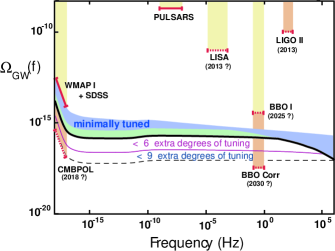
Figure 6: The figure taken from Ref. [52] shows the theoretical predictions and observational constraints on primordial gravitational waves from inflation. The gravitational wave energy density per logarithmic frequency interval, (in units of the critical density) is plotted versus frequency. The shaded (blue) band labeled ‘minimally tuned’ represents the range predicted for simple inflation models with the minimal number of parameters and tunings. The dashed curves have lower values of tensor contribution, $r$, that is possible with more fine tuned inflationary scenarios. The currently existing experimental constraints shown are due to: big bang nucleosynthesis (BBN), binary pulsars, and WMAP-1 (first year) with SDSS. Also shown are the projections for LIGO (both LIGO-I, after one year running, and LIGO-II); LISA; and BBO (both initial sensitivity, BBO-I, and after cross-correlating receivers, BBO-Corr). Also seen the projected sensitivity of a future space mission for CMB polarization (CMBPol).

On large angular scales, the curl component of CMB polarization is a unique signature of tensor perturbations. Hence, the CMB B-polarization is a direct probe of the energy scale of early universe physics that generate the primordial metric perturbations (scalar & tensor). The relative amplitude of tensor to scalar perturbations, $r$, sets the energy scale for inflation ${\cal E}_{\rm Inf}=3.4\times 10^{16}$ GeV $r^{1/4}$. A measurement of $B$–mode polarization on large scales would give us this amplitude, and hence a direct determination of the energy scale of inflation. Besides being a generic prediction of inflation, the cosmological gravity wave background from inflation would be a fundamental test of GR on cosmic scales and the semi–classical behavior of gravity. Figure 6 summarizes the current theoretical understanding, observational constraints and future possibilities for the stochastic gravity wave background from Inflation.

6 Conclusions

The past few years has seen the emergence of a ‘concordant’ cosmological model that is consistent both with observational constraints from the background evolution of the universe as well that from the formation of large sale structures. It is certainly fair to say that the present edifice of the ‘standard’ cosmological models is robust. A set of foundation and pillars of cosmology have emerged and are each supported by a number of distinct observations [53].

The community is now looking beyond the estimation of parameters of a working ‘standard’ model of cosmology. There is increasing effort towards establishing the basic principles and assumptions. The feasibility and promise of this ambitious goal is based on the grand success in the recent years in pinpointing a ‘standard’ model. The up coming results from the Planck space mission will radically improve the CMB polarization measurements. There are already proposals for the next generation dedicated satellite mission in 2020 for CMB polarization measurements at best achievable sensitivity.

References

- [1] T. Souradeep, J. R. Bond, L. Knox, G. Efstathiou, M. S. Turner, Prospects for measuring Inflation parameters with the CMB in Proc. of COSMO97, Sept 15-19, 1997, Ambleside, UK; ed. L. Roszkowski, (World Scientific, Singapore 1998) (astro-ph/9802282).
- [2] A. Shafieloo, T. Souradeep, preprint arXiv:0901.0716.
- [3] D. Larson et al., preprint , (arXiv:1001.4635); E. Komatsu et al., preprint , (arXiv:1001.4638).
- [4] M. L. Brown et al., ,Astrophys. J., 705, 798 (2009).
- [5] C. L. Reichardt et al., Astrophys. J., 694, 1200 (2009); S. Das et al.,preprint arXiv:1009.0847
- [6] R. Saha, P, Jain & T. Souradeep, Astrophys. J. Lett., 645, L89, (2006); P. Samal et al., Astrophys.J. 714, 840, (2010).
- [7] D. Spergel et al., Astrophys.J.Suppl, 170, 377, (2007).
- [8] J. R. Bond and G. Efstathiou ApJ 285 L45 (1984); W. Hu and M. White New Astron. 2 323 (1997).
- [9] G. B. Rybicki and A. P. Lightman Radiative processes in astrophysics (New York: Wiley–Interscience, 1979).
- [10] J. M. Kovac et al., Nature 420, 772, (2002).
- [11] L. Page et al., Astrophys.J.Suppl., 170, 335, (2007).
- [12] A. Kogut, et.al., Astrophys.J.Suppl., 148, 161 (2003).
- [13] E.Y.S. Wu et al. Phys.Rev.Lett. 102,161302,(2009).
- [14] A. Lue, L. Wang and M. Kamionkowski Phys. Rev. Lett. 83, 1506, (1999); D. Maity, P. Majumdar and S. SenGupta JCAP 0406 005 (2004).
- [15] J. R. Bond, D. Pogosyan, & T. Souradeep,, Class. Quant. Grav. 15, 2671 (1998); ibid. Phys. Rev. D 62,043005 (2000); Phys. Rev. D 62,043006 (2000).
- [16] M. Tegmark, A. de Oliveira-Costa, & A. Hamilton Phys.Rev. D68 123523 (2004).
- [17] C. J. Copi, D. Huterer, & G. D. Starkman, Phys. Rev. D. 70 043515, (2004).
- [18] D. J. Schwarz et al., Phys. Rev. Lett. 93, 221301 (2004).
- [19] H. K. Eriksen et al., Astrophys. J 605, 14 (2004).
- [20] D. L. Larson & B. D. Wandelt, Astrophys. J. Lett. 613, L85 (2004).
- [21] G. Hinshaw et al., Astrophys.J.Suppl. 170, 288, (2007).
- [22] C. L. Bennett et al., preprint, arXiv:1001.4758 [WMAP-7].
- [23] A. Hajian, & T. Souradeep, Astrophys. J. Lett. 597, L5 (2003); A. Hajian, T. Souradeep & N. Cornish, Astrophys. J. Lett. 618, L63 (2005).
- [24] A. Hajian & T. Souradeep,Phys.Rev. D74 123521 (2006).
- [25] S. Basak, A. Hajian, T. Souradeep, Phys. Rev. D 74 021301(R) (2006).
- [26] D. J. Eisenstein, et al., Astrophys.J. 633, 560 (2005).
- [27] S. Coles et al. Mon.Not.Roy.Astron.Soc. 362, 505 (2005).
- [28] P. J. E. Peebles & J. T. Yu, Astrophys. J. 162, 815 (1970).
- [29] R.A. Sunyaev, & Ya.B. Zel’dovich, Astr. Space Science, 7, 3 (1970).
- [30] J.R. Bond, & G. Efstathiou, Astrophys. J., 285, L45 (1984).
- [31] J.R. Bond, & G. Efstathiou, MNRAS, 226, 655, (1987).
- [32] J.A. Holtzmann, Astrophys.J.Suppl., 71, 1 (1989).
- [33] A. A. Starobinsky, Phys. Lett, 117B, 175 (1982); A. H. Guth, & S.-Y. Pi, Phys. Rev. Lett., 49, 1110 (1982); J. M. Bardeen, P. J. Steinhardt, & M. S. Turner, Phys. Rev. D 28, 679 (1983).
- [34] G. F. Smoot et al., Astrophys. J. Lett. 396, L1, (1992).
- [35] C. L. Bennett et al., Astrophys.J.Suppl. 148, 1, (2003).
- [36] N. Kogo, M. Matsumiya, M. Sasaki, J. Yokoyama Astrophys.J. 607 32 (2004).
- [37] S. L. Bridle et. al., Mon.Not.Roy.Astron.Soc. 342 L72 (2003).
- [38] S. Hannestad, JCAP, 0404, 002 (2004).
- [39] P. Mukherjee and Y. Wang, Astrophys.J. 599 1 (2003).
- [40] P. Mukherjee and Y. Wang, JCAP 0512 007 (2005).
- [41] M. Tegmark and M. Zaldarriaga, Phys. Rev. D66, 103508, (2002).
- [42] M. Matsumiya, M. Sasaki, J. Yokoyama, Phys.Rev. D65, 083007, (2002); ibid, JCAP 0302 003 (2003).
- [43] A. Shafieloo and T. Souradeep, Phys Rev. D 70, 043523, (2004).
- [44] D. Tocchini-Valentini, M. Douspis, J. Silk, MNRAS 359 31 (2005).
- [45] R. Sinha and T. Souradeep, Phys.Rev. D 74 043518 (2006).
- [46] R.K. Jain et al., JCAP, 0901, 009,(2009).
- [47] A. Shafieloo et al., Phys.Rev.D75:123502,(2007)
- [48] J. Hamann, A. Shafieloo, T. Souradeep, JCAP 1004:010,(2010).
- [49] D. Munshi, T. Souradeep and A. Starobinsky, Astrophysical Journal, 454, 552, (1995).
- [50] D. N. Spergel, D. M. Goldberg, Phys.Rev. D59 103001 (1999).
- [51] C. J. MacTavish et al., Astrophys. J 647, 799 (2006).
- [52] L. A. Boyle, P. J. Steinhardt & N. Turok, Phys. Rev. Lett. 96 111301 (2006).
- [53] J. P. Ostriker and T. Souradeep, Pramana, 63, 817, (2004).