The Milky Way stellar halo out to 40 kpc : Squashed, broken but smooth

Abstract

We introduce a new maximum likelihood method to model the density profile of Blue Horizontal Branch and Blue Straggler stars and apply it to the Sloan Digital Sky Survey Data Release 8 (DR8) photometric catalogue. There are a large number ($\sim$ 20,000) of these tracers available over an impressive $14,000$ deg² in both Northern and Southern Galactic hemispheres, and they provide a robust measurement of the shape of the Milky Way stellar halo. After masking out stars in the vicinity of the Virgo Overdensity and the Sagittarius stream, the data are consistent with a smooth, oblate stellar halo with a density that follows a broken power-law. The best fitting model has an inner slope $\alpha_{\rm in}\sim 2.3$ and an outer slope $\alpha_{\rm out}\sim 4.6$, together with a break radius occurring at $\sim 27$ kpc and a constant halo flattening (that is, ratio of minor axis to major axis) of $q\sim 0.6$. Although a broken power-law describes the density fall-off most adequately, it is also well fit by an Einasto profile. There is no strong evidence for variations in flattening with radius, or for triaxiality of the stellar halo.

1 Introduction

The time required for stars in the stellar halo to exchange their energy and angular momentum is very long compared to the age of the Galaxy. Therefore, such stars preserve memories of their initial conditions, and so the structure of the stellar halo is intimately linked to the formation mechanism of the Galaxy itself. This fundamental insight was already noted by Eggen et al. (1962). It is the reason why the stellar halo has attracted such interest despite containing only a small fraction of the total stellar mass of the Galaxy. Stars diffuse more quickly in configuration space, as opposed to energy and angular momentum space. So, the spatial structure of the stellar halo may be smooth, even though it is built up from merging and accretion.

The simplest way of studying the stellar halo is through starcounts. Typically, RR Lyrae or blue horizontal branch stars (BHBs) are used as tracers, as they are relatively bright ($M_{g}\sim 0.5-0.7$, e.g. Sirko et al. 2004) and can be detected at radii out to $\sim$ 100 kpc. The gathering of such data is painstaking work, and carries the price that sample sizes are often small. Such studies are consistent with a stellar halo that is round in the outskirts (with a minor-to-major axis ratio $q=1$) and more flattened in the inner parts with $q\sim 0.5$ (e.g., Hartwick 1987; Preston et al. 1991). Rather than selecting typical halo stars, an alternative approach is to model deep star count data in pencil-beam surveys at intermediate and high galactic latitudes, allowing for contamination of the starcounts by the thin and thick disk populations. This was attempted by Robin et al. (2000), who found a best-fit halo density law with flattening $q\sim 0.76$, together with a power-law fall-off $\alpha$ of $2.4$ (that is, $\rho\sim({\rm distance)}^{-\alpha}$). A similar, slightly later, attempt by Siegel et al. (2002) using data in seven Kapteyn selected areas yielded $q\sim 0.6$ and $\alpha\sim 2.75$.

Efforts to detect variations in the flattening with radius have also been undertaken. Preston et al. (1991) argued that the flattening changes from strongly flattened ($q=0.5$) at 1 kpc to almost round at $20$ kpc. However, work by Sluis & Arnold (1998) using a compilation of 340 RR Lyraes and BHBs found a constant flattening of $q\sim 0.5$ with no evidence for changes with radius, as well as and a power-law index $\alpha\sim-3.2$. The most recent work by De Propris et al. (2010) utilising 666 BHB stars from the 2dF Quasar Redshift Survey find that the halo is approximately spherical with a power-law index of $\alpha=2.5$ out to $\sim 100$ kpc. Similarly, Sesar et al. (2011) studying Main Sequence Turn-Off (MSTO) stars from the Canada-France-Hawaii Telescope Legacy Survey find that the flattening is approximately constant at $q\sim 0.7$ out to $35$ kpc.

The Sloan Digital Sky Survey (SDSS) has transformed our knowledge of the stellar halo. Although it had been suspected that the stellar halo is criss-crossed with streams and substructures ever since the discovery of the disrupting Sagittarius (Sgr), the SDSS provided a memorable picture of the debris in The Field of Streams (Belokurov et al. 2006). A wealth of substructure has now been identified, including the Sagittarius stream, the Virgo Overdensity and the Hercules-Aquila Cloud (e.g. Ibata et al. 1995; Belokurov et al. 2006; Jurić et al. 2008; Belokurov et al. 2007). This has been seen as vindication of modern theories of galaxy formation, which predict that stellar haloes are built up almost exclusively from the debris of disrupting satellites (e.g. Bullock & Johnston 2005; De Lucia & Helmi 2008; Cooper et al. 2010). A number of studies have attempted to model the smooth halo component by avoiding these known substructures (e.g. Jurić et al. 2008). The results are only in very rough agreement, suggesting that the density profile of the Milky Way has a power-law slope in the range $2<\alpha<4$ and a flattening varying from $0.4<q<0.8$ (e.g. Yanny et al. 2000; Chen et al. 2001; Newberg & Yanny 2006; Jurić et al. 2008; Sesar et al. 2011).

Even though panoramic photometric surveys like SDSS do provide a large sample of stellar halo tracers over a considerable portion of the sky, there is no consensus on the flattening and shape of the stellar halo. MSTO stars are commonly used tracers owing to their large numbers and the ease by which they can be photometrically identified (e.g. Bell et al. 2008). The absolute magnitudes of such stars centre around $M_{r}\sim 4.5$ but have a wide range of values ($\sigma_{M_{r}}\sim 0.9$ mag) which limits the accuracy to which the density profile can be estimated. BHB stars are superior distance estimators ($\sigma_{M_{r}}\sim 0.15$), but are significantly scarcer than main sequence stars. Moreover, they suffer from contamination by blue straggler (BS) stars due to their similar colours. BHB and BS stars can be distinguished by their Balmer line profiles (e.g. Kinman et al. 1994; Yanny et al. 2000; Sirko et al. 2004; Clewley et al. 2002), but this requires spectroscopic information. Whilst spectroscopic samples can cleanly identify BHB stars, the variety of results on flattening (e.g., Preston et al. 1991; Sluis & Arnold 1998; De Propris et al. 2010) and density fall-off (e.g. Xue et al. 2008; Brown et al. 2010) suggests that the completeness biases are difficult to understand and control.

An independent constraint on the density profile of the stellar halo is provided by the velocity distribution of the halo stars. A kinematic analysis by Carollo et al. (2007) (see also Carollo et al. 2010) suggests that the stellar halo comprises of two components with different density profiles and metallicities. The authors find that the density profile becomes shallower beyond $15-20$ kpc. This is in stark contrast to the studies by Watkins et al. (2009) and Sesar et al. (2010), who find a significantly steeper density profile beyond $\sim 30$ kpc from the distribution of RR Lyrae stars in SDSS Stripe 82. A caveat to the interpretation of kinematic studies is that the density distribution is not measured directly but rather modelled by assuming a dark matter halo potential.

Therefore, the present state-of-play is distressingly inconclusive and a further attack on the problem of the shape of the stellar halo is warranted. In this study, we introduce a new method to model both BHB and BS stars based on photometric information alone. We make use of the SDSS DR8 photometric data release which has now mapped an impressive $\sim 14,000$ deg² of sky with both Northern and Southern coverage. In contrast to previous work, we combine both the wide sky coverage of the SDSS with the accurate distance estimates provided by the BHB stars to model the density profile of the stellar halo out to $\sim 40$ kpc.

The paper is arranged as follows. In §2.1, we describe the SDSS DR8 photometric data and our selection criteria for A-type stars. The remainder of §2 introduces the probability distribution for BHB and BS membership based on colour alone and outlines the absolute magnitude-colour relations for the two populations. In §4, we describe our maximum likelihood method to determine the density profile of the stellar halo and in §4 we present our results. Finally, we draw our main conclusions in §5.

2 A-type stars in SDSS Data Release 8

2.1 Data Release 8 (DR8) Imaging

The Sloan Digital Sky Survey (SDSS; York et al. 2000) is an imaging and spectroscopic survey covering roughly $\sim 1/4$ of the sky. Imaging data is obtained using a CCD camera (Gunn et al. 1998) on a 2.5 m telescope (Gunn et al. 2006) at Apache Point Observatory, New Mexico. Images are obtained simultaneously in five broad optical bands ($ugriz$; Fukugita et al. 1996). The data are processed through pipelines to measure photometric and astrometric properties (Lupton et al. 2001; Smith et al. 2002; Stoughton et al. 2002; Pier et al. 2003; Ivezić et al. 2004; Tucker et al. 2006). The SDSS DR8 release contains all of the imaging data taken by the SDSS imaging camera and covers over $\sim 14,000$ deg² of sky (Aihara et al. 2011). We select objects classified as stars with clean photometry. The magnitudes and colours we use in the following sections have been corrected for extinction following the prescription of Schlegel et al. (1998).

In the top panel of Fig. 1, we show the sky coverage of SDSS data release 8 (DR8) in equatorial coordinates. For comparison, the sky coverage of the SDSS data release 5 (DR5) is indicated by the darker grey region. The more recent SDSS data release covers both Northern and Southern latitudes. We exclude latitudes $|b|<30^{\circ}$, so as to concentrate on regions well away from the plane of the galaxy. Over the distance range probed by this work, the SDSS footprint ($|b|>30^{\circ}$) covers approximately 20% of the total volume of the stellar halo. In this study we use blue horizontal branch (BHB) and blue straggler stars (BS) to map the density profile of the stellar halo. These A-type stars are selected by choosing stars in the following region in colour-colour space:

$$0.9<u\!-\!g<1.4$$

$$-0.25<g\!-\!r<0.0$$ (1)

This selection is similar to other work using A-type stars (e.g. Yanny et al. 2000; Sirko et al. 2004) and is chosen to exclude main sequence stars, white dwarfs and QSOs. The bottom left hand panel of Fig. 1 highlights the colour selection box. Whilst we assume that all of our selected stars are BHBs or BSs, there may be a non-negligible contribution by variable stars, such as RR Lyrae. We use multi-epoch stripe 82 data to estimate the fraction of variable stars in the same magnitude and colour range as our sample. We use the light curve catalogue compiled by Bramich et al. (2008) and classify variable stars according to the criteria outlined in Sesar et al. (2007). The resulting fraction of variable stars is $\sim 5\%$. This small fraction of non-BHB and non-BS stars will therefore make little difference to the results of this work.

In the bottom right hand panel of Fig. 1, we show the error in $u\!-\!g$ and $g\!-\!r$ colours as a function of $g$ band magnitude. The photometric errors in $u\!-\!g$ are larger than in $g\!-\!r$, especially at fainter magnitudes. This can be compared with the typical separation between BHBs and BS stars in $u\!-\!g$ colour (see bottom panel of Figure 2) which ranges from 0.05 to 0.1 mag. Mean photometric error $\sigma_{(u\!-\!g)}$ reaches 0.05 at $g\sim 18.5$ and beyond that the value rapidly increases. Accordingly, in this study we only select stars in the magnitude range $16<g<18.5$. This corresponds to a distance range of $\sim 4-40$ kpc for typical absolute magnitudes of BHB and BS stars. Note that BHB and BS stars have different absolute magnitudes, and so span separate, but overlapping, distance ranges (see Section 2.3).

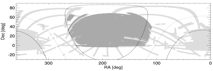
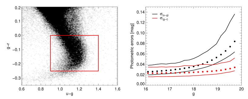
Figure 1: Top panel: The SDSS DR8 footprint in equatorial coordinates. The solid and dotted lines show $|b|=30^{\circ}$ and $b=0^{\circ}$ respectively. The darker grey area shows the sky coverage of the SDSS data release 5 (DR5). The more recent DR8 sample has both Northern and Southern sky coverage. Bottom left panel: The colour selection in $u\!-\!g$ and $g\!-\!r$ used to select BHB and BS stars. Our sample consists of $N=20290$ stars in the magnitude range $16<g<18.5$. Bottom right panel: The median (dots), 5th and 95th percentiles of the photometric error in $u\!-\!g$ (black) and $g\!-\!r$ (red) colours as a function of $g$ band magnitude. Beyond $g\sim 18.5$, the errors in $u\!-\!g$ increase fairly rapidly.

2.2 Ridgelines in Colour-Colour Space

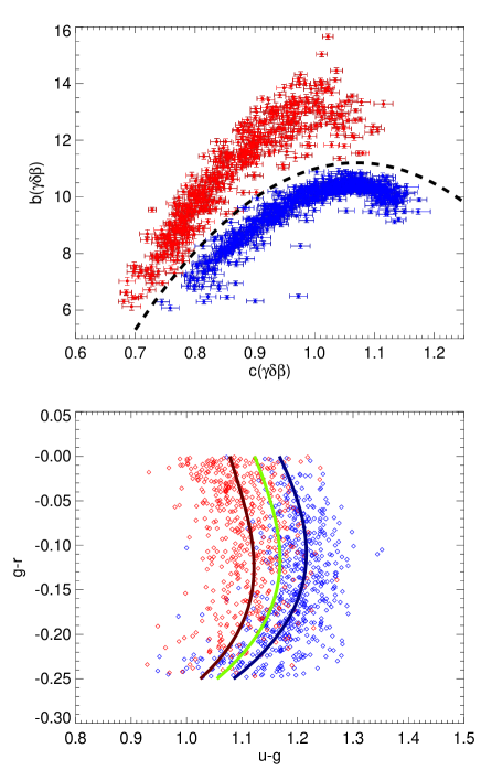
Figure 2: Top panel: The scale width, $b(\gamma\delta\beta)$, and line shape, $c(\gamma\delta\beta)$, of the Balmer lines $H_{\gamma}$, $H_{\delta}$ and $H_{\beta}$ for bright A-type stars taken from the SDSS data release 7 (DR7) spectral catalogue. These stars are selected in the same colour range as our DR8 photometric sample and have magnitudes in the range $16<g<17$. The blue and red points denote BHB and BS stars respectively. The black dashed line shows the apparent separation of these stars based on the Sersic line profiles of the Balmer series. Bottom panel: The ‘ridgelines’ for the BHB and BS stars in the colour space ($u\!-\!g,g\!-\!r$). The thick blue and red lines show the third order polynomial fits to these loci in colour space. The green line indicates the approximate border between the two populations.

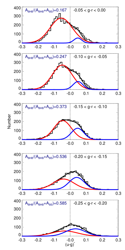
Figure 3: The distribution of colours in $\left(u\!-\!g\right)^{\star}$ space. Each row shows the distribution for a different range in $g\!-\!r$ colour. A two component model is fit to the data. The overall model is shown by the black line. Individual Gaussians are shown by the red (BS) and blue (BHB) lines respectively. Stars with $\left(u\!-\!g\right)^{\star}<0$ are dominated by BS stars whilst stars with $\left(u\!-\!g\right)^{\star}>0$ are dominated by BHB stars. The ratio between the amplitude of the Gaussians gives an estimate of the overall number ratio between the two populations.

We seek to measure the centroids of the BHB and BS loci in colour space as well as their intrinsic widths. Naturally, this can only be done provided there exists a robust classification of the A-type stars according to their surface gravity. It has been shown (e.g. Clewley et al. 2002; Sirko et al. 2004; Xue et al. 2008) that BHB and BS stars can be separated cleanly on the basis of their Balmer line profiles. We proceed by selecting A-type stars from the spectral SDSS data release 7 (DR7) catalogue within the same colour range as our DR8 photometric sample. Restricting the sample to high signal-to-noise (S/N) spectra in the magnitude range $16<g<17$, we fit the Balmer lines $H_{\gamma}$, $H_{\delta}$ and $H_{\beta}$ with Sersic profile of the form,

$$y=1.0-a\,\exp-\left(\frac{|x-x_{0}|}{b}\right)^{c},$$ (2)

where $x_{0}$ and $a$ give the wavelength and the line depth at the line centre respectively. The parameters $b$ (the scale width) and $c$ are related to the line width and line shape respectively. The relation between combined line widths and line shapes of the three Balmer lines $H_{\gamma}$, $H_{\delta}$ and $H_{\beta}$ are shown in the top panel of Fig. 2. The BHBs (blue points) and BSs (red points) are clearly separated in this diagram and the decision boundary is indicated by the dashed black line. We use this spectral classification to pinpoint the loci of the two populations in the $u\!-\!g,g\!-\!r$ colour-colour space. In our analysis, these “ridgelines”, i.e. approximate centres in $u\!-\!g$ as a function of $g\!-\!r$, are defined by third order polynomials:

$$(u\!-\!g)^{0}_{\rm BHB} = 1.167-0.775(g\!-\!r)-1.934(g\!-\!r)^{2}$$

$$+9.936(g\!-\!r)^{3},$$

$$(u\!-\!g)^{0}_{\rm BS} = 1.078-0.489(g\!-\!r)+0.556(g\!-\!r)^{2}$$ (3)

$$+13.444(g\!-\!r)^{3},$$

for $-0.25<g\!-\!r<0.0$. The ridgelines are shown by the thick blue and red lines in the bottom panel of Fig. 2. The green line indicates the approximate boundary between BHBs and BSs in $u\!-\!g$, $g\!-\!r$ space. In addition, we calculate the intrinsic spread of the two populations about their ridgelines. We find $\sigma_{\rm BHB,0}(u\!-\!g)=0.04$ and $\sigma_{\rm BS,0}(u\!-\!g)=0.045$. Fig. 2 makes it apparent that, even for brightest stars, photometric information alone is not enough to separate BHB and BS stars. Therefore, for a given star we define the probability of BHB or BS class membership based on its distance in colour-colour space from the appropriate locus. We assume that both populations are distributed in a Gaussian manner about their ridgelines. We model the conditional probability of measuring $u\!-\!g$ and $g\!-\!r$ colours, given the star of each species, as

$$p(ugr~{}|~{}{\rm BHB})\propto\mathrm{exp}\left(-\frac{\left[(u\!-\!g)-(u\!-\!g)_{\rm BHB}^{0}\right]^{2}}{2\sigma_{\rm BHB}^{2}}\right),$$

$$p(ugr~{}|~{}{\rm BS})\propto\mathrm{exp}\left(-\frac{\left[(u\!-\!g)-(u\!-\!g)_{\rm BS}^{0}\right]^{2}}{2\sigma_{\rm BS}^{2}}\right).$$ (4)

Note that, in fact, these probabilities are also functions of $g\!-\!r$ since the centre of the Gaussian distribution, $(u\!-\!g)^{0}$ varies with the $g\!-\!r$ colour (see eqn. 2.2). The dispersion about the ridgeline centre depends on the intrinsic width and the photometric errors in $u\!-\!g$, $\sigma=\sqrt{\sigma^{2}_{0}+\sigma_{(u\!-\!g)}^{2}}$. The colour-based posterior probabilities of class membership are then

$$P({\rm BHB}~{}|~{}ugr)=\frac{p(ugr~{}|~{}{\rm BHB})~{}N_{\rm BHB}}{p(ugr~{}|~{}{\rm BHB})~{}N_{\rm BHB}+p(ugr~{}|~{}{\rm BS})~{}N_{\rm BS}}$$

$$P({\rm BS}~{}|~{}ugr)=\frac{p(ugr~{}|~{}{\rm BS})~{}N_{\rm BS}}{p(ugr~{}|~{}{\rm BHB})~{}N_{\rm BHB}+p(ugr~{}|~{}{\rm BS})~{}N_{\rm BS}}$$ (5)

The total numbers of stars $N_{\rm BHB}$ and $N_{\rm BS}$ in a given colour range can then be found iteratively by integrating equations (2.2). In Table 1, we give the fraction of BHB and BS stars in five $g\!-\!r$ colour bins. The fraction ranges from $f_{\rm BHB}\sim 0.15$ at redder colours to $f_{\rm BHB}\sim 0.6$ at bluer colours. This is in good agreement with the overall BHB to BS ratios estimated by Bell et al. (2010) and Xue et al. (2008) who use similar magnitude ranges.

	$N_{\rm tot}$	$f_{\rm BHB}$	$f_{\rm BS}$
$-0.05<g\!-\!r<0.00$	5189	0.154	0.846
$-0.10<g\!-\!r<-0.05$	4973	0.231	0.769
$-0.15<g\!-\!r<-0.10$	4151	0.346	0.654
$-0.20<g\!-\!r<-0.15$	3564	0.536	0.464
$-0.25<g\!-\!r<-0.20$	2413	0.613	0.387

Table 1: The fraction of BHB and BS stars in different colour bins. We give the $g\!-\!r$ colour range, the total number of stars, the estimated fraction of BHB stars and the estimated fraction of BS stars.

Figure 3 demonstrates the evolution of the separation between the two populations in colour space. For illustration purposes, the SDSS $u\!-\!g$ colour is transformed into $\left(u\!-\!g\right)^{\star}$ using the following relation:

$$\left(u\!-\!g\right)^{\star}=(u\!-\!g)-(u\!-\!g)^{0}_{\rm border}$$ (6)

Here, $(u\!-\!g)^{0}_{\rm border}=1.223-0.632(g\!-\!r)-0.689(g\!-\!r)^{2}+11.690(g\!-\!r)^{3}$ is defined by the approximate boundary line between BHB and BS stars shown by the green line in Fig. 2. In these new coordinates, the curved shape of the decision boundary becomes a straight line. In Fig. 3, we fit two Gaussian distributions to the distribution in $\left(u\!-\!g\right)^{\star}$ for five bins in $g\!-\!r$. This two component model fits the overall distribution very well. The ratio between the amplitudes of the two Gaussians varies with $g\!-\!r$ colour. The fraction of BHB stars increases towards bluer colours, in good agreement with our estimates in Table 1.

2.3 Absolute Magnitudes

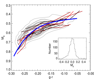
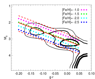
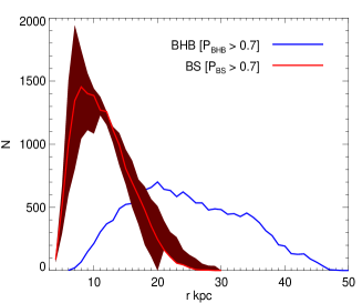
Figure 4: Left Panel: The colour-absolute magnitude relation for BHB stars derived from star clusters published in An et al. (2008). A polynomial of order 4 is fit to the BHB stars in eleven star clusters: M2, M3, M5, M13, M53, M92, NGC2419, NGC4147, NGC5053 and NGC5466 (solid blue line). The grey contours indicate the density of stars within the colour-absolute magnitude region (thicker lines indicate higher densities). The ridgelines for individual clusters are shown by the red/black lines. These are colour coded by metallicity: red to black goes from more metal rich ([Fe/H]   -1.3) to more metal poor ([Fe/H]   -2.3). The inset panel shows the distribution of values around the derived relation indicating a small degree of scatter. Middle panel: The density of BS stars in Stripe 82 belonging to the Sagittarius stream. The solid and dashed red lines give the absolute magnitude colour relation and the estimated dispersion ($\sigma_{M_{g}}\sim 0.5$). The distance to this portion of the Sagittarius stream is estimated from Watkins et al. (2009) as $D_{\rm Sgr}=26.1\pm 5.6$ kpc. The coloured dots show the relation derived by Kinman et al. (1994) for different metallicity BS stars in star clusters. Right panel: The radial distribution of the BHB and BS star populations. The blue line shows the distribution for high probability BHB stars ($P(\mathrm{BHB})>0.7$). The red shaded region shows the distribution for high probability BS stars ($P(\mathrm{BS})>0.7$) where the uncertainty in the absolute magnitudes is taken into account.

Let us now derive a relationship between the absolute magnitude and colour of BHB and BS stars. BHB stars are intrinsically brighter and their absolute magnitude varies little as a function of temperature (colour) or metallicity. In comparison, BS are intrinsically fainter and span a much wider range in absolute magnitude.

The absolute magnitudes of BHB stars are calibrated using star clusters with SDSS photometry published by An et al. (2008). Ten star clusters have prominent BHB sequences; M2, M3, M5, M13, M53, M92, NGC2419, NGC4147, NGC5053 and NGC5466. The density distribution of absolute magnitudes of BHB stars in these clusters is shown as a function of $g\!-\!r$ colour in the left hand panel of Fig. 4. There is little variation of the absolute magnitude with colour for BHB stars. $M_{g}$ changes by 0.2 (from 0.65 to 0.45) in the $-0.25<g\!-\!r<0$ range. The inset panel shows the variation of absolute magnitude about the $M_{g(\rm BHB)}$ vs. $g\!-\!r$ trend ($M_{g}^{*}$). The spread of this distribution is $\sim 0.1$, indicating that there is a tight relation describing the BHB absolute magnitude. The star clusters have metallicities typical of halo stars and ranging from $-2.3<[\mathrm{Fe/H}]<-1.3$, but we find no obvious trend with metallicity.

BS stars are less common in globular clusters than BHB stars. Instead, to calibrate the absolute magnitudes of BS stars we make use of stars in Stripe 82 belonging to the Sagittarius stream. The distance to the stream in the right ascension range $25^{\circ}<\alpha^{\circ}<40^{\circ}$ was estimated by Watkins et al. (2009) using RR Lyrae stars as $D_{\rm Sgr}=26.1\pm 5.6$ kpc. In the middle panel of Fig. 4, we show the absolute magnitude of stars in Stripe 82 between $25^{\circ}<\alpha^{\circ}<40^{\circ}$ as a function of colour. The density contours are constructed by using stars outside of the range in right ascension as a background and computing the density contrast. An obvious plume of BS stars is apparent in the density plot. This is shown by the contour levels extending off the main sequence. The solid red line shows the estimated absolute magnitude colour relation for these BS stars. For comparison, we show the absolute magnitude versus colour relation for BS stars estimated by Kinman et al. (1994). This relation is converted from Johnson-Cousins photometry ($UBV$) to Sloan photometry ($ugr$) using the transformation derived in Jester et al. (2005). The different coloured dots show the relation for different metallicity stars. The absolute magnitude calibration derived for the BS stars in the Sagittarius stream is almost identical to the Kinman et al. (1994) relation for BS stars with metallicity $[\mathrm{Fe/H}]=-1.5$. This is in good agreement with the metallicity of the stream stars found by Watkins et al. (2009) ($[\mathrm{Fe/H}]=-1.43$).

We compute the spread of absolute magnitudes for each colour bin as $\sigma_{M_{g}}\sim 0.5$. This dispersion takes into account the distance errors ($D_{\rm Sgr}=26.1\pm 5.6$ kpc) and encompasses a range of metallicities (see dashed red lines in Fig. 4). Hence, we conclude that our calibration for BS absolute magnitudes does not have a strong metallicity bias. Note that the ‘average’ BS absolute magnitude is $\sim 2.5$, approximately $2$ magnitudes fainter than the BHB stars. This is entirely consistent with the absolute magnitudes of halo BS stars found by Yanny et al. (2000) and Clewley et al. (2004).

The resulting absolute magnitudes of BHB and BS stars as a function of $g\!-\!r$ colour are:

$$M_{g(\rm BHB)} = 0.434-0.169(g\!-\!r)+2.319(g\!-\!r)^{2}$$

$$+20.449(g\!-\!r)^{3}+94.517(g\!-\!r)^{4},$$

$$M_{g(\rm BS)} = 3.108+5.495(g\!-\!r),$$ (7)

which are valid over the colour range $-0.25<g\!-\!r<0.0$. For BHB stars, this allows us to estimate accurately the distances of BHB candidates. For BS stars, the relation is only approximate and the scatter for each colour interval needs to be taken into account for all distance estimates.

In the right hand panel of Fig. 4, we show the estimated radial distributions for the BHB and BS populations. We select high probability BHB and BS stars by using the membership probabilities defined in eqn. (2.2). ‘High’ probability BHB/BS stars are defined as those for which we are $68\%$ (or $1\sigma$) confident of BHB/BS membership. The BHB stars probe a radial range from $r\sim 10$ kpc to $r\sim 45$ kpc. BS stars, which have fainter absolute magnitudes, only probe out to $\sim 30$ kpc. However, there is a large degree of overlap between the two populations between $10$ and $30$ kpc.

3 Maximum Likelihood Method

In this section, we outline the maximum likelihood method used to constrain the density profile of the stellar halo. An important assumptions in the modelling is that the BHB and BS stars follow the same density distribution, modulo an overall scaling. The number of BHB stars and BS stars in a given increment of magnitude and area on the sky is then described by

$$\Delta N_{\rm BHB}(m_{g}\!-\!M^{\rm BHB}_{g},\ell,b) = \rho^{0}_{\rm BHB}\rho(m_{g}\!-\!M^{\rm BHB}_{g},\ell,b)D^{3}_{\rm BHB}$$

$$\quad\times\,\frac{1}{5}\mathrm{ln}10\,\Delta m_{g}\,\mathrm{cos}b\,\Delta\ell\,\Delta b$$

$$\Delta N_{\rm BS}(m_{g}\!-\!M^{\rm BS}_{g},\ell,b) = \rho^{0}_{\rm BS}\rho(m_{g}\!-\!M^{\rm BS}_{g},\ell,b)D^{3}_{\rm BS}$$

$$\quad\times\,\frac{1}{5}\mathrm{ln}10\,\Delta m_{g}\,\mathrm{cos}b\,\Delta\ell\,\Delta b.$$

Here, the distance increment $\Delta D$ has been converted into the apparent magnitude increment via the relation $\Delta D=\frac{1}{5}\mathrm{ln}10\,D\Delta m_{g}$. The normalising factors, $\rho^{0}_{\rm BHB}=N_{\rm BHB}/V_{\rm BHB}$ and $\rho^{0}_{\rm BS}=N_{\rm BS}/V_{\rm BS}$ are found by performing volume integrals over the SDSS DR8 sky coverage and over the required magnitude range

$$V_{\rm BHB}(M^{\rm BHB}_{g}) = \int\int\int\left[\rho(m_{g}-M^{\rm BHB}_{g},\ell,b)D_{\rm BHB}^{3}\right.$$

$$\qquad\qquad\qquad\left.\times\,\frac{1}{5}\mathrm{ln}10\,\mathrm{d}m_{g}\,\mathrm{cos}b\,\mathrm{d}\ell\,\mathrm{d}b\right]$$

$$V_{\rm BS}(M^{\rm BS}_{g}) = \int\int\int\left[\rho(m_{g}-M^{\rm BS}_{g},\ell,b)D_{\rm BS}^{3}\right.$$ (9)

$$\qquad\qquad\qquad\left.\times\,\frac{1}{5}\mathrm{ln}10\,\mathrm{d}m_{g}\,\mathrm{cos}b\,\mathrm{d}\ell\,\mathrm{d}b\right].$$

These normalising integrals depend on the absolute magnitude of the stars and hence on the $g\!-\!r$ colour ($M_{g}=M_{g}(g\!-\!r)$ from eqn. 2.3). Note that the values of $V_{\rm BHB}$ and $V_{\rm BS}$ play a minor role in identifying the maximum likelihood model given the choice of parameters, but are important when evaluating the performances of different model families. We also assume that our sample consists only of BHB and BS stars so the total number of stars is the sum of these two populations, $N_{\rm tot}=N_{\rm BHB}+N_{\rm BS}$ where $N_{\rm BHB}=f_{\rm BHB}N_{\rm tot}$ and $N_{\rm BS}=f_{\rm BS}N_{\rm tot}$. The overall fraction of BHB to BS stars varies as a function of $g\!-\!r$ colour, as shown in the previous section.

Combining equations (2.2) and (3) gives the number of stars in a cell of colour, magnitude, longitude and latitude space

$$\Delta N = p(ugr~{}|~{}{\rm BHB})\Delta N_{\rm BHB}+p(ugr~{}|~{}{\rm BS})\Delta N_{\rm BS}$$ (10)

$$= N_{\rm tot}\nu(ugr,l,b)\Delta(g\!-\!r)\Delta m_{g}\Delta\ell\Delta b\mathrm{cos}b\frac{1}{5}\mathrm{ln}10,$$

where the stellar density is

$$\nu(ugr,l,b) = p(ugr~{}|~{}{\rm BHB})\frac{f_{\rm BHB}}{V_{\rm BHB}}\rho(m_{g}\!-\!M^{\rm BHB}_{g},\ell,b)D^{3}_{\rm BHB}+$$ (11)

$$p(ugr~{}|~{}{\rm BS})\frac{f_{\rm BS}}{V_{\rm BS}}\rho(m_{g}\!-\!M^{\rm BS}_{g},\ell,b)D^{3}_{\rm BS}$$

Here, each star is assigned a ‘BHB distance’ ($D_{\rm BHB}$) as well as a ‘BS distance’ ($D_{\rm BS}$). The colour probability functions weight the contribution of each star to the BHB density or the BS density. For simplicity, we group all the stars into five bins in $g\!-\!r$ of width 0.05 mags. Thus, stars in each $g\!-\!r$ bin have the same normalisations ($V_{\rm BHB}$, $V_{\rm BS}$), fraction of BHB/BS stars ($f_{\rm BHB}$, $f_{\rm BS}$) and absolute magnitudes ($M^{\rm BHB}_{g}$, $M^{\rm BS}_{g}$). We take into account the uncertainty in the BS absolute magnitude by convolving the BS number density with a Gaussian magnitude distribution. This distribution is centred on the estimated absolute magnitude ($M^{\rm BS}_{g}=M^{\rm BS}_{g}(g\!-\!r)$) and has a dispersion of $\sigma_{M_{g}}=0.5$ (see Fig. 4).

The log-likelihood function can then be constructed from the density distribution,

$$\mathrm{log}\mathcal{L}=\sum_{i=1}^{N_{\rm tot}}\mathrm{log}\,\left[\nu(m^{i}_{g},ugr^{i},\ell^{i},b^{i})~{}\mathrm{cos}b\right].$$ (12)

The number of free parameters constrained by the likelihood function depends on the complexity of the model stellar-halo density profile. The log-likelihood is maximised to find the best-fit parameters using a brute-force grid search.

$N_{\rm tot}$	$\alpha$	$q$	$\mathrm{ln}(\mathcal{L})\times 10^{4}$	$\sigma/\rm tot$	with V&S?
20290	$2.60^{+0.05}_{-0.05}$	$0.65^{+0.02}_{-0.02}$	-17.1171	$0.38\pm 0.01$	yes
15403	$2.90^{+0.05}_{-0.1}$	$0.53^{+0.02}_{-0.01}$	-12.2917	$0.22\pm 0.02$	no

Table 2: A summary of our best-fit oblate power-law models with and without the Virgo Overdensity and the Sagittarius stream. We give the total number of stars, the model parameters, the average log-likelihood value for the model and $\sigma/\rm tot$.

4 Results

In this section, we outline the results of applying our maximum likelihood method to the sample of A-type stars selected from the SDSS DR8. We consider in turn a number of simple density profiles with constant flattening – single power-law, broken power-law and Einasto – before examining the case for refinements, such as triaxiality, radial variations in shape and substructure.

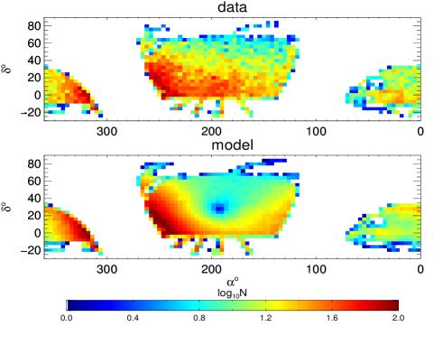
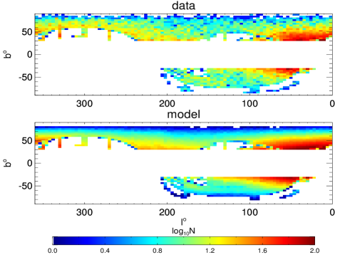
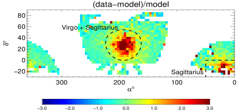
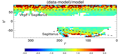
Figure 5: Left panels: Density plots in equatorial coordinates. Right panels: Density plots in Galactic coordinates. The top and middle panels show the density plots for the the data and single power-law model respectively. The bottom panels show the residuals of the best-fit single power-law model. The dark red regions show the obvious overdensities of Virgo and Sagittarius. The dashed lines indicate the regions of sky removed in the maximum likelihood procedure. The Virgo Overdensity and parts of the leading tail of the Sagittarius stream are apparent in the North Galactic Cap whereas another portion of the Sagittarius stream is found in the South Galactic Cap. Note that these have been excised when calculating the best-fit single power-law model. The regions away from these known overdensities are reasonably well fit by a smooth, power-law density model.

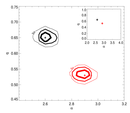
Figure 6: The maximum likelihood contours for the flattening $q$ and power-law index $\alpha$ of our single power-law halo models. The black (red) lines show the $1\sigma$, $2\sigma$ and $3\sigma$ contours when stars in the region of the Virgo overdensity and Sagittarius stream have been included (excluded). The inset panel illustrates that the difference in maximum likelihood parameters is relatively small whether the overdensities are included or excluded.

4.1 Single Power-Law Profile

First, let us consider a simple power-law density model of the form,

$$\rho(r_{q})\propto r_{q}^{-\alpha},\qquad\qquad r_{q}^{2}=x^{2}+y^{2}+z^{2}q^{-2}$$ (13)

The parameters $q$ and $\alpha$ describe the halo flattening and the power-law fall-off in stellar density respectively. Oblate density distributions have $q<1$, spherical $q=1$ and prolate $q>1$.

Figure 7: Likelihood contours for the broken power-law models. Left panel: The contours for the inner ($\alpha_{\rm in}$) and outer ($\alpha_{\rm out}$) power laws. The fall off steepens at larger radii. Right panel: The contours for the break radius ($r_{\rm b}$) and flattening ($q$). The maximum likelihood solution favours a flattening of $q=0.59$ and a break radius of $r_{\rm b}=27$ kpc with inner and outer power-laws of $\alpha_{\rm in}=2.3$ and $\alpha_{\rm out}=4.6$ respectively.

We summarise the best-fitting single power-law model parameters in Table 2. Using the entire sample, we find the maximum likelihood model parameters of $\alpha=2.6$ and $q=0.65$. We repeat the analysis by excising stars in the regions of the Virgo Overdensity and Sagittarius stream, which amounts to removing stars in the regions defined by

$$0<X<30,\quad\quad X=63.63961\sqrt{2(1-\sin b)}.$$ (14)

This is the mask introduced by Bell et al. (2008) to remove stars belonging to the Virgo overdensity (as well as parts of the leading tail of the Sagittarius stream). Another portion of the Sagittarius stream is located in the Southern part of the sky (see Fig. 5) and is removed by

$$0^{\circ}<\alpha<50^{\circ},\quad-30^{\circ}<\delta<0^{\circ}.$$ (15)

By discarding these large overdensities, we find a slightly steeper power law and a more flattened shape with $\alpha=2.9$ and $q=0.53$. There is also a substantial increase in the maximum likelihood, implying that the fit is indeed affected by the presence of these large overdensities. In Fig  6, we show the maximum likelihood contours for the model parameters $q$ and $\alpha$ for both cases. The contours encompass the $1\sigma$, $2\sigma$ and $3\sigma$ regions respectively. We find that our likelihood function has a well defined peak. The maximum likelihood model parameters ($\alpha=2.9$, $q=0.53$ excluding overdensities) are in good agreement with some of the previous work assuming a single power-law model for the stellar halo (e.g. Yanny et al. 2000; Newberg & Yanny 2006; Jurić et al. 2008). This exercise indicates that the two large overdensities induce a bias in deduced model parameters and, therefore, in the subsequent sections, we remove stars in the vicinity of the Virgo Overdensity and Sagittarius stream in all our calculations.

We use our maximum likelihood smooth oblate halo model ($\alpha=2.9$, $q=0.53$) to show the residuals of the data minus model on the sky. In Fig. 5, we compare the data and model in both equatorial and galactic coordinates. The top and middle panels show the data and model on the sky (the magnitude distribution has been collapsed) whilst the bottom panels show the residuals of the model. The Virgo overdensity is the most obvious feature located at ($\alpha\sim 190^{\circ}$, $\delta\sim 30^{\circ}$). This overdensity covers a substantial fraction of the North Galactic cap. A portion of the Sagittarius stream can be seen at ($\alpha\sim 20^{\circ}$, $\delta\sim-25^{\circ}$) in the South Galactic cap. The residuals for these features reach up to approximately three times the model values. We can estimate the total fraction of stars residing in these overdensities from the excess numbers of stars in these regions of the sky. Approximately $\sim 5.5\%$ of our total sample ($N_{\rm tot}=20290$) reside in the Northern Virgo+Sagittarius overdensity whilst less than $1\%$ occupy the Southern portion of the Sagittarius stream. The fraction of stars in these overdensities is relatively small as they are located in the vicinity of the Northern and Southern Galactic caps where the density of stars is small. However, as the relative difference (i.e. (data-model)/model) between the data and model is large in these regions, these overdensities can influence the likelihood values.

4.2 Broken Power-Law Profile

We relax our models to allow a change in the steepness of the density fall off and consider broken power-law models of the form,

$$\rho(r_{q})\propto\begin{cases}r_{q}^{-\alpha_{\rm in}}&r_{q}\leq r_{\rm b}\\ r_{q}^{-\alpha_{\rm out}}&r_{q}>r_{\rm b}.\end{cases}$$ (16)

In Fig. 7 we show the maximum likelihood contours for the inner and outer power-laws (left hand panel) and break radii and flattening (right hand panel). A model with break radius $r_{\rm b}=27$ kpc is preferred with slopes of $\alpha_{\rm in}=2.3$, $\alpha_{\rm out}=4.6$ respectively. A steeper power-law is favoured at larger radii while the power-law within the break radius is shallower. Note that the break radius is an ellipsoidal distance and only corresponds to a radial Galactocentric distance in the Galactic plane ($z=0$). The model is slightly less flattened ($q\sim 0.6$) than the single power-law model but, even with an additional two parameters, an oblate halo model is favoured.

The maximum likelihood value for a broken power-law model is significantly larger than for a single power-law model ($-2\mathrm{ln}(\mathcal{L}_{\rm SPL}/\mathcal{L}_{\rm BPL})\sim 400$) (see Table 3). Our broken power-law model is in very good agreement agreement with the results of Watkins et al. (2009), who use a sample of RR Lyrae stars to probe the density distribution of the stellar halo out to $\sim 100$ kpc (see also Sesar et al. 2010).

Figure 8: The magnitude distribution of our DR8 data sample. The black points give the distribution of the data where the error bars are Poissonian. Top-left panel: Single power-law models. The solid and dashed red lines show the best fit oblate and spherical models respectively. Error bars incorporate Poissonian uncertainties and the spread of absolute magnitudes for BS stars. A flattened model provides a much better fit to the data. Top-right panel: The solid red, blue and green lines show the distributions for the best-fit single power-law, broken power-law and Einasto models respectively. The latter two provide a better representation of the data. Bottom-left panel: The magnitude distribution for the most probable BHB stars (with $P_{\rm BHB}>0.7$). Bottom-right panel: The magnitude distribution for the most probable BS stars (with $P_{\rm BS}>0.7$).

4.3 Einasto Profile

The Einasto profile (Einasto & Haud 1989) is often used to describe the density distribution of dark matter haloes (e.g. Graham et al. 2006; Merritt et al. 2006; Navarro et al. 2010). The Einasto model is given by the equation

$$\mathrm{ln}\left[\rho(r_{q})/\rho(r_{\rm eff})\right]=-d_{n}[(r_{q}/r_{\rm eff})^{1/n}-1].$$ (17)

The shape of the density profile is described by the parameter $n$. Density distributions with steeper inner profiles and shallower outer profiles are generated by large values of $n$. For example, dark matter haloes with ‘cuspy’ inner profiles typically have values of $n\sim 6$. The parameter $d_{n}$ is a function of $n$. For $n\geq 0.5$ a good approximation is given by $d_{n}=3n-1/3+0.0079/n$ (Graham et al. 2006).

This profile allows for a non-constant fall-off without the need for imposing a discontinuous break radii. We find the maximum likelihood solutions for $q$, $n$ and $r_{\rm eff}$. Our best-fit Einasto model has parameters $q=0.58$, $n=1.7$ and $r_{\rm eff}=20$ kpc. The slope of the density profile varies rapidly with radius as indicated by the relatively small value of $n$.

4.4 Model Comparisons

We now test how accurately our models represent the observed magnitude distribution of the data. Using Monte Carlo methods, we create a distance distribution according to the model density profile. The fake data is given a $g\!-\!r$ colour distribution drawn from the real data, which can then be converted into absolute magnitudes (see eqn. 2.3). The ratio of BHB and BS stars in each colour bin is chosen to match the values given in Table 1. In the case of the BS stars, absolute magnitudes are determined from the $g\!-\!r$ colour by drawing randomly from a Gaussian distribution centered on the estimated value (from eqn. 2.3) with a dispersion of 0.5 mags. The resulting (apparent) magnitude distributions for our models are compared with the data in Fig. 8

In the top-left hand panel, we show the magnitude distribution for our single power-law oblate model with the solid red line. The error bars take into account the Poisson uncertainty as well as the uncertainty spread of absolute magnitudes for BS stars. The distribution of magnitudes for our DR8 A-type star sample is shown by the black points. There is reasonably good agreement but there is a notable deviation at fainter magnitudes. For comparison, we show the maximum likelihood spherical model by the red dashed line (with $\alpha\sim 2.7$), which provides a very poor fit to the data. The top-right hand panel shows the magnitude distributions for the single power-law, broken power-law and Einasto profiles by the solid red, blue and green lines respectively. The broken power-law and Einasto models provide a better representation of the data than a single power-law, although there are still discrepancies at the faintest magnitudes.

In the bottom panels of Fig. 8, we show the magnitude distributions for the most probable BHB and BS stars. We select stars with $P_{\rm BHB}>0.7$ as ‘BHB’ stars and stars with $P_{\rm BS}>0.7$ as ‘BS’ stars (see section 2.3). Of course, this is for illustration purposes only, as a clean separation of BHB and BS stars requires spectroscopic classification. While the BS stars are adequately described by a single power-law model, this is a poor description of the BHB stars. This is unsurprising, as the BS stars cover a smaller distance range and barely populate distances beyond the break radius. The bottom-left panel clearly shows the need for a more steeply declining density law at larger radii.

In Fig.  9, we show the distribution of (probable) BHB stars in spherical shells with the solid black line. Here, we only consider the most likely BHB stars (with $P_{\rm BHB}>0.7$) as for these we can accurately estimate their distance. The red, blue and green lines show the radial distributions for our best fit single power-law, broken power-law and Einasto models respectively. The single power-law is a poorer description of the data, whilst the broken power-law and Einasto models both provide better representations of the radial distribution.

Figure 9: Left panel: The number of BHB stars in spherical shells. We select stars with $P(\rm BHB)>0.7$ as ‘BHB’ stars and show their radial distribution with the thick black line. The solid blue, red and green lines show our best-fit broken power-law, single power-law and Einasto models respectively. Right panel: The residuals for our best fit models.

Model	Parameters	$N_{p}$	$\mathrm{ln}(\mathcal{L})\times 10^{4}$	$-2\mathrm{ln}(\mathcal{L}_{\rm max}/\mathcal{L})$	$\mathrm{ln}(E/E_{\mathrm{max}})$	$\sigma/\rm tot$ (w/o V & S)	$\sigma/\rm tot$ (V & S)
SPL - spherical	$\alpha=2.7^{+0.05}_{-0.05}$, $\mathbf{q=1.0}$	1	-12.5516	5606	-2801	$0.44\pm 0.01$	$0.49\pm 0.01$
SPL - oblate	$\alpha=2.9^{+0.04}_{-0.06}$, $q=0.53^{+0.02}_{-0.01}$	2	-12.2917	408	-206	$0.22\pm 0.02$	$0.38\pm 0.01$
SPL - triaxial	$\alpha=2.9^{+0.05}_{-0.05}$, $q=0.50^{+0.02}_{-0.01}$, $p=0.71^{+0.03}_{-0.03}$	3	-12.2818	210	-110	$0.20\pm 0.02$	$0.34\pm 0.01$
SPL - $q=q(r)$	$\alpha=2.9^{+0.05}_{-0.05}$, $q=0.53^{+0.02}_{-0.01}$, $r_{0}>10^{3}$kpc	3	-12.2917	368	-206	$0.22\pm 0.02$	$0.38\pm 0.01$
BPL - oblate	$r_{b}=27^{+1}_{-1}$kpc, $q=0.59^{+0.02}_{-0.03}$,	4	-12.2713	0	0	$0.21\pm 0.02$	$0.36\pm 0.01$
	$\alpha_{\rm in}=2.3^{+0.1}_{-0.1}$, $\alpha_{\rm out}=4.6^{+0.2}_{-0.1}$
Einasto - oblate	$n=1.7^{+0.2}_{-0.2}$, $r_{\rm eff}=20^{+1.0}_{-1.0}$kpc, $q=0.58^{+0.02}_{-0.02}$	3	-12.2757	88	-45	$0.22\pm 0.01$	$0.37\pm 0.01$

Table 3: A summary of our best-fit models. We give the type of model, the best-fit parameters of the model, the number of free parameters, the maximum log-likelihood, the difference in likelihood relative to the maximum likelihood model, the log evidence¹ ratio relative to the maximum likelihood model and $\sigma/\rm tot$ both with and without the Virgo and Sagittarius overdensities. Parameters which are kept fixed are highlighted in bold.

4.5 Refinements: Triaxiality and a Radially Dependent Shape

A natural question to ask is whether further refinements might provide a still more accurate description of the data. Up to now, we have assumed spheroidal halo models with a constant flattening with radius.

First, we consider whether triaxiality makes any improvement. The definition of $r_{q}$ is modified to

$$r_{q}^{2}=x^{2}+y^{2}p^{-2}+z^{2}q^{-2}.$$ (18)

We fit single power-law triaxial models to the data and obtain maximum likelihood parameters of $q=0.50$ and $p=0.71$. The likelihood value increases relative to an oblate model with the inclusion of this extra parameter ($-2\mathrm{ln}(\mathcal{L}_{\rm oblate}/\mathcal{L}_{\rm triaxial})\sim 200$). The magnitude distribution of the triaxial model is largely the same as the oblate model. We inspect the difference between these two models in equatorial coordinates in Fig. 10. The dot-dashed lines indicates the regions of sky with low galactic latitudes $|b|<40^{\circ}$. Regions with latitudes below $|b|<30^{\circ}$ have been removed. The triaxial model is notably overdense relative to the oblate model in the regions centered on $(\alpha,\delta)=(125^{\circ},50^{\circ})$ and $(\alpha,\delta)=(60^{\circ},10^{\circ})$. The latter region, located in the Southern part of the sky, is close to the portion of the Sagittarius stream excised in our best fit model. The former is coincident with the Monocerus ring (Newberg et al. 2002), which can be identified, for example, in Figure 1 of Belokurov et al. (2006). We suggest that the apparent triaxiality may well be caused by the presence of these overdensities. The increased flexibility of the model can cause it to ‘fit’ to such substructure and thus the increase in likelihood may be an artifact.

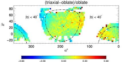
Figure 10: The residuals of our maximum likelihood triaxial and oblate models. The dot-dashed region indicates the boundary between low ($|b|<40^{\circ}$) and high ($|b|<40^{\circ}$) Galactic latitudes. Note the difference in scale that is used for this figure to that used for Fig. 5.

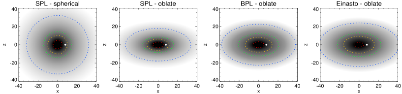
Figure 11: A side view of our maximum likelihood models. Greyscale shows density of stars in plane of Galactocentric $(x,z)$ at $y=0$ in four maximum-likelihood models. The blue, green, yellow and red contours show density levels corresponding to the 50th, 90th, 95th and 99th percentiles of the spherical model. The white dot marks the location of the Sun.

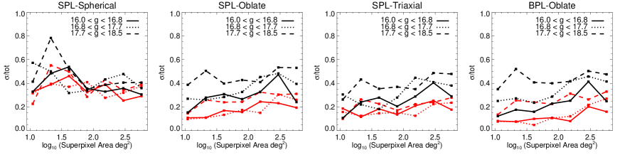
Figure 12: The scale dependence of substructure. We show the $\sigma/\mathrm{tot}$ fraction as a function of superpixel size. Individual panels show the relation for our various maximum likelihood models. The different line styles indicate different magnitude bins. The black lines show the relation for all the stars. The red lines show the relation when stars in the vicinity of the Virgo overdensity and Sagittarius have been removed.

Some earlier investigations have found evidence that the shape of the stellar halo changes from a flattened distribution at smaller radii to an almost spherical distribution at larger radii (e.g. Preston et al. 1991). We can test this claim by allowing the flattening $q$ to vary with radius. Following the reasoning of Sluis & Arnold (1998), we make the following substitution

$$q\rightarrow q\sqrt{\frac{r^{2}+r^{2}_{0}}{q^{2}r^{2}+r_{0}^{2}}}$$ (19)

The halo flattening is still $q$ at small radii but tends to sphericity at large radii. The scale radius $r_{0}$ determines the radial range over which this change occurs. For example, for large values of $r_{0}$ (e.g. larger than the most distant stars) the flattening is approximately constant over the applicable radial range. We fit single power-law models with a varying flattening to the data and find that large scale radii are preferred ($r_{0}>10^{3}$ kpc) with an inner flattening of $q=0.53$. This indicates that the flattening is approximately constant over the radial range of the data (out to $\sim 40$ kpc). This is in agreement with the deductions of Sluis & Arnold (1998) and Sesar et al. (2011), who also found no real evidence for a varying shape with radius.

In summary, we find that the data are well described by an oblate density distribution with a constant flattening of $q\sim 0.6$ and a more steeply declining profile at larger radii. We summarise our maximum likelihood models by giving a ‘side view’ of the profiles in Fig. 11. A spherical model is strongly disfavoured whereas oblate broken power-law and Einasto models provide a good representation.

Our best-fit density distribution can be used to estimate the total stellar mass. We find the total number of BHB stars by integrating the BHB density profile over all space in the distance range $1-40$kpc. The number of BHB stars can be converted into a total Luminosity using the relation derived in Deason et al. (2011) using globular clusters: $N_{\rm BHB}/L\sim 10^{-3}$. Assuming a mass-to-light ratio of $M/L\sim 1-5$, the stellar mass is approximately $2-10\times 10^{8}M_{\odot}$. Bell et al. (2008) calculate a total stellar mass of $\sim 3.7\times 10^{8}M_{\odot}$ using main sequence stars, in good agreement with our estimate. Note that the total stellar halo mass is believed to be $\sim 10^{9}M_{\odot}$ (e.g. Morrison et al 1993) so we are probing a significant fraction of the stellar halo ($\sim 20-100\%$).

4.6 The Amount of Substructure

A rough idea of the amount of substructure present in the data can be attained by computing the rms deviation of the models about the data ($\sigma/\mathrm{tot}$) as defined by equations (2) and (3) in Bell et al. (2008):

$$\langle\sigma^{2}\rangle=\frac{1}{n}\sum_{k}\left(D_{k}-M_{k}\right)^{2}-\frac{1}{n}\sum_{k}\left(M^{{}^{\prime}}_{k}-M_{k}\right)^{2},$$ (20)

$$\frac{\sigma}{\mathrm{tot}}={\langle\sigma^{2}\rangle^{1/2}\over(1/n)\sum_{k}D_{k}}.$$ (21)

Here, $D_{k}$ is the number of stars in bin $k$, $M_{k}$ is the expected number from the model, $M^{{}^{\prime}}_{k}$ is a Poisson random deviate from the model value and $n$ is the total number of bins (in $l$, $b$ and $m_{g}$). However, with a total of $\sim 20,000$ stars we can not afford to use a fixed bin size over the entire sky: pixels must be simultaneously large enough to contain ample stars and small enough to adequately sample the substructure. To circumvent this problem, we use the Voronoi binning method of Cappellari & Copin (2003) to partition the data in pixels on the sky. This adaptive binning method groups pixels together, forming ‘superpixels’, with the objective of obtaining a constant signal-to-noise ratio per bin. We choose the signal-to-noise ratio of $S/N\sim 4$ (assuming Poisson noise) to ensure the mean number of stars in each 2D bin is $\gtrsim 10$. We also check that our results are not affected by the choice of signal-to-noise. The stars are split into three $g$ band magnitude ranges, binned into $\sim 65,000$ $1^{\circ}\times 1^{\circ}$ pixels for full sky coverage which are then combined into $\sim 750$ superpixels using the procedure described above to estimate the overall $\sigma/\mathrm{tot}$ values. These are given in the last two columns of Table 3. As expected, our $\sigma/\mathrm{tot}$ fraction is significantly reduced when the stars in the region of the Virgo Overdensity and Sagittarius stream are removed: the estimated fraction of substructure reduces from $40\%$ to $20\%$. However, further refinement of our model makes little difference to the $\sigma/\mathrm{tot}$ fraction, even if the likelihood is increased. This is indicative of the resilience of our maximum likelihood method to relatively minor amounts of substructure present in the data.

We illustrate the dependence of $\sigma/\mathrm{tot}$ on spatial scale in Fig. 12 by grouping together superpixels with similar spatial scales and computing $\sigma/\mathrm{tot}$ for each group. This shows how the fraction of substructure depends on the superpixel size (in $\mathrm{deg}^{2}$) for different maximum likelihood models. $\sigma/\mathrm{tot}$ is computed both with (black lines) and without (red lines) the stars in the vicinity of the Virgo Overdensity and the Sagittarius stream. The spherical model has relatively large values of $\sigma/\mathrm{tot}$ over all scales, illustrating the poor fit of this model to the data. The single and broken power-law oblate models show a scale dependence, whereby larger scales (larger number of pixels) have an increased $\sigma/\mathrm{tot}$ fraction relative to smaller scales. Similar behaviour is also true for the triaxial model but the $\sigma/\mathrm{tot}$ fractions are slightly lower. As alluded to earlier, we suspect that this may be caused by the triaxial model describing some of the large-scale substructure (namely the Monocerus ring or parts of the Sagittarius stream which have not been excised).

Different lines in Fig. 12 show the dependence of the $\sigma/\mathrm{tot}$ measure on the apparent magnitude of the tracers and hence correspond to different distances probed. The slight rise of the rms with magnitude indicates that higher fractions of substructure may be present at larger distances. This can be simply explained with the increase of the substructure lifetime with radius as governed by the orbital period of the infalling Galactic fragments.

When interpreting these plots, it is important to bear in mind that the smallest superpixels are biased towards the densest parts of the halo, while the emptiest regions are sampled by the largest agglomerations of 2D bins. This bias could potentially explain at least some of the trend with size. On the scales smaller than several tens of degrees, $\sigma/\mathrm{tot}$ in our models is in the range $0.05<\sigma/\mathrm{tot}<0.2$ indicating that the halo is not dominated by substructure and is relatively smooth. While there is evidence that the fraction of substructure increases with scale, this apparent increase in $\sigma/\mathrm{tot}$ could also be caused by spurious pixels. In sparse regions, the grouping of many pixels, each containing very few stars, poses a limitation to this method.

5 Conclusions

We have developed a new method to simultaneously model the density profile of both blue horizontal branch (BHB) and blue straggler (BS) stars based on their broad-band photometry alone. The probability of BHB or BS membership is defined by the locus of these stars in $u\!-\!g$, $g\!-\!r$ space. We use these colour-based weights to construct the overall probability function for the density of the two populations. When applied to the A-type stars selected from the Sloan Digital Sky Survey (SDSS) Data Release 8 (DR8) photometric catalog, the best-fit stellar halo models are identified by applying a maximum likelihood algorithm to the data.

Based on the data from regions with $30^{\circ}<|b|<70^{\circ}$, we find that the stellar halo is not spherical in shape, but flattened. Spherical models cannot reproduce the distribution of the A-type stars in our sample and are discrepant with the data at both bright and faint magnitudes. Our best-fit models suggest that the stellar halo is oblate with a flattening (or minor axis to major axis ratio) of $q=0.59$ with a typical uncertainty of $\sigma_{q}\sim 0.1$. As a simple representation of the stellar halo, we advocate the use of a broken power-law model with an inner slope $\alpha_{\rm in}=2.3$ and an outer slope $\alpha_{\rm out}=4.6$, the break radius occurring at about 27 kpc. This gives the formula

$$\rho(r_{q})\propto\begin{cases}r_{q}^{-2.3}&r_{q}\leq 27\ {\rm kpc},\\ r_{q}^{-4.6}&r_{q}>27\ {\rm kpc},\end{cases}$$ (22)

with $r_{q}^{2}=R^{2}+z^{2}/0.59^{2}$. For those who prefer Einasto models, an equally good law for the stellar halo density is

$$\rho(r_{q})\propto\exp\left[-4.77[(r_{q}/20{\rm kpc})^{1/1.7}-1]\right].$$ (23)

These two formulae are fundamental results of our paper, and can be summarised as the Milky Way stellar halo is squashed and broken. The results are qualitatively similar to those obtained by Sesar et al. (2011) using main-sequence stars. There is no evidence in the data for variation of the flattening with radius. There is some mild evidence for a triaxial shape, but the apparent triaxiality might be due to the presence of the Monocerus ring at low latitudes ($|b|<40^{\circ}$) and regions of the Southern Sagittarius stream.

The root-mean-square deviation of the data around the maximum likelihood model $\sigma/\mathrm{tot}$ typically ranges between $5\%$ and $20\%$. This indicates that the Milky Way stellar halo, or at least the component traced by the A-type stars in the SDSS DR8, is smooth and not dominated by unrelaxed substructure.

This finding is discrepant with the conclusions of Bell et al. (2008). These authors use main sequence turn-off stars selected from SDSS data release 5 (DR5) to model the stellar halo density. They argue that no smooth model can describe the data and conclude that the stellar halo is dominated by substructure (with $\sigma/\mathrm{tot}\geq 0.33$). We suggest that these contrasting results may be due to the different methods and tracers used. Bell et al. (2008) search for the lowest $\sigma/\mathrm{tot}$ fraction models. However, we find that the $\sigma/\mathrm{tot}$ values very little between different density models even if the likelihood is substantially increased. Furthermore, a lower $\sigma/\mathrm{tot}$ could also indicate that a model is ‘fitting’ to any substructure (e.g. triaxial models both in this work and in Bell et al. 2008). Bell et al. (2008) also use main sequence stars as tracers which are more numerous than A-type stars, but are much poorer distance indicators. The adopted absolute magnitude scale for main sequence stars is dependent on metallicity and colour. Bell et al. (2008) assume a median absolute magnitude of $M_{r}\sim 4.5$ with a scatter of $\sigma_{M_{r}}=0.9$; an appropriate choice for a halo population with metallicity $[\mathrm{Fe/H}]\sim-1.5$. The scatter, even with an assumed metallicity, is greater than the spread in absolute magnitude for BS stars ($\sigma_{M_{g}}\sim 0.5$ per colour bin). Uncertainties in the distances to stars could lead to compact substructures becoming more blurred out over a wider range of distance. It is possible that Bell et al. (2008) see a somewhat younger and/or metal-richer component of the stellar halo with the main sequence tracers. This component could be more unrelaxed than the one traced by A type stars.

Our conclusion that the stellar halo is composed of a smooth underlying density, together with some additional substructures such as the Virgo Overdensity and the Sagittarius Stream, is very reassuring. If the stellar halo were merely a hotch-potch of tidal streams and unrelaxed substructures, then modelling and estimation of total mass and potential would be much more difficult. Many of the commonly-used tools of stellar dynamics – such as the steady-state Jeans equations – implicitly assume a well-mixed and smooth equilibrium. This raises the hope that a full understanding of the spatial and kinematic properties of stars in the smooth, yet squashed and broken, stellar halo can yield the gravitational potential and dark matter profile of the Galaxy itself.

References

- Aihara et al. (2011) Aihara H., et al., 2011, ArXiv e-prints
- An et al. (2008) An D., et al., 2008, ApJS, 179, 326
- Bell et al. (2008) Bell E. F., et al., 2008, ApJ, 680, 295
- Bell et al. (2010) Bell E. F., Xue X. X., Rix H., Ruhland C., Hogg D. W., 2010, AJ, 140, 1850
- Belokurov et al. (2006) Belokurov V., et al., 2006, ApJ, 642, L137
- Belokurov et al. (2007) Belokurov, V., et al. 2007, ApJ, 657, L89
- Bramich et al. (2008) Bramich, D.M., et al. 2008, MNRAS, 386, 887
- Brown et al. (2010) Brown W. R., Geller M.J., Kenyon S. J., Diaferio A., 2010, ApJ, 139, 59
- Bullock & Johnston (2005) Bullock J. S., Johnston K. V., 2005, ApJ, 635, 931
- Cappellari & Copin (2003) Cappellari M., Copin Y., 2003, MNRAS, 342, 345
- Carollo et al. (2007) Carollo D., et al., 2007, Nature, 450, 1020
- Carollo et al. (2010) Carollo D., et al., 2010, ApJ, 712, 692
- Chen et al. (2001) Chen B., et al., 2001, ApJ, 553, 184
- Chiba & Beers (2000) Chiba M., Beers T. C., 2000, AJ, 119, 2843
- Clewley et al. (2004) Clewley L., Warren S. J., Hewett P. C., Norris J. E., Evans N. W., 2004, MNRAS, 352, 285
- Clewley et al. (2002) Clewley L., Warren S. J., Hewett P. C., Norris J. E., Peterson R. C., Evans N. W., 2002, MNRAS, 337, 87
- Cooper et al. (2010) Cooper A. P., et al., 2010, MNRAS, 406, 744
- Deason et al. (2011) Deason A. J., Belokurov V., Evans N. W., 2011, MNRAS, 411, 1480
- De Lucia & Helmi (2008) De Lucia G., Helmi A., 2008, MNRAS, 391, 14
- De Propris et al. (2010) De Propris R., Harrison C. D., Mares P. J., 2010, ApJ, 719, 1582
- Eggen et al. (1962) Eggen O. J., Lynden-Bell D., Sandage A. R., 1962, ApJ, 136, 748
- Einasto & Haud (1989) Einasto J., Haud U., 1989, A&A, 223, 89
- Font et al. (2011) Font A. S., McCarthy I. G., Crain R. A., Theuns T., Schaye J., Wiersma R. P. C., Dalla Vecchia C., 2011, ArXiv e-prints
- Fukugita et al. (1996) Fukugita M., Ichikawa T., Gunn J. E., Doi M., Shimasaku K., Schneider D. P., 1996, AJ, 111, 1748
- Graham et al. (2006) Graham A. W., Merritt D., Moore B., Diemand J., Terzić B., 2006, AJ, 132, 2701
- Gunn et al. (1998) Gunn J. E., et al., 1998, AJ, 116, 3040
- Gunn et al. (2006) Gunn J. E., et al., 2006, AJ, 131, 2332
- Hartwick (1987) Hartwick F. D. A., 1987,in Gilmore G., Carswell B., eds, The Galaxy. Reidel, Dordrecht , p. 281
- Ibata et al. (1995) Ibata R. A., Gilmore G., Irwin M. J., 1995, MNRAS, 277, 781
- Ivezić et al. (2004) Ivezić v. Z., et al., 2004, Astron Nach, 325, 583
- Jester et al. (2005) Jester S., et al., 2005, AJ, 130, 873
- Jurić et al. (2008) Jurić M., et al., 2008, ApJ, 673, 864
- Keller et al. (2008) Keller S. C., Murphy S., Prior S., Da Costa G., Schmidt B., 2008, ApJ, 678, 851
- Kinman et al. (1994) Kinman T. D., Suntzeff N. B., Kraft R. P., 1994, AJ, 108, 1722
- Lupton et al. (2001) Lupton R., Gunn J. E., Ivezić Z., Knapp G. R., Kent S., 2001 Vol. 238 of ASP Conf. Ser., Astronomical data analysis software and systems x. p. 269
- Merritt et al. (2006) Merritt D., Graham A. W., Moore B., Diemand J., Terzić B., 2006, AJ, 132, 2685
- Morrison et al (1993) Morrison H. L., 1993,AJ,106,578
- Navarro et al. (2010) Navarro J. F., et al., 2010, MNRAS, 402, 21
- Newberg et al. (2002) Newberg H. J., et al., 2002, ApJ, 569, 245
- Newberg & Yanny (2006) Newberg H. J., Yanny B., 2006, Journal of Physics Conference Series, 47, 195
- Pier et al. (2003) Pier J. R., Munn J. A., Hindsley R. B., Hennessy G. S., Kent S. M., Lupton R. H., Ivezić Ž., 2003, AJ, 125, 1559
- Preston et al. (1991) Preston G. W., Shectman S. A., Beers T. C., 1991, ApJ, 375, 121
- Robin et al. (2000) Robin A. C., Reylé C., Crézé M., 2000, A&A, 359, 103
- Schlegel et al. (1998) Schlegel D. J., Finkbeiner D. P., Davis M., 1998, ApJ, 500, 525
- Searle & Zinn (1978) Searle L., Zinn R., 1978, ApJ, 225, 357
- Sesar et al. (2007) Sesar B., et al., 2007, ApJ, 134, 2236
- Sesar et al. (2010) Sesar B., et al., 2010, ApJ, 708, 717
- Sesar et al. (2011) Sesar B., Juric M., Ivezic Z., 2011, ApJ, 731, 4
- Siegel et al. (2002) Siegel M. H., Majewski S. R., Reid I. N., Thompson I. B., 2002, ApJ, 578, 151
- Sirko et al. (2004) Sirko E., et al., 2004, AJ, 127, 899
- Sluis & Arnold (1998) Sluis A. P. N., Arnold R. A., 1998, MNRAS, 297, 732
- Smith et al. (2002) Smith J. A., et al., 2002, AJ, 123, 2121
- Stoughton et al. (2002) Stoughton C., et al., 2002, AJ, 123, 485
- Tucker et al. (2006) Tucker D. L., et al., 2006, Astronomische Nachrichten, 327, 821
- Watkins et al. (2009) Watkins L. L., et al., 2009, MNRAS, 398, 1757
- Xue et al. (2008) Xue X. X., et al., 2008, ApJ, 684, 1143
- Xue et al. (2010) Xue X. X., et al., 2010, ArXiv e-prints
- Yanny et al. (2000) Yanny B., et al., 2000, ApJ, 540, 825
- York et al. (2000) York D. G., et al., 2000, AJ, 120, 1579
- Zolotov et al. (2010) Zolotov A., Willman B., Brooks A. M., Governato F., Hogg D. W., Shen S., Wadsley J., 2010, ApJ, 721, 738