Abstract

In the context of non overlapping domain decomposition methods, several algebraic approximations of the Dirichlet-to-Neumann (DtN) map are proposed in [F. X. Roux, et. al.Algebraic approximation of Dirichlet-to-Neumann maps for the equations of linear elasticity, Comput. Methods Appl. Mech. Engrg., 195, 2006, 3742-3759]. For the case of non overlapping domains, approximation to the DtN are analogous to the approximation of the Schur complements in the incomplete multilevel block factorization.

In this work, several original and purely algebraic (based on graph of the matrix) domain decomposition techniques are investigated for steady state incompressible Navier-Stokes equation defined on uniform and stretched grid for low viscosity. Moreover, the methods proposed are highly parallel during both setup and application phase. Spectral and numerical analysis of the methods are also presented.

1 Introduction

At the core of some numerical simulations lies the problem of solving sparse linear systems of the form

$$\mathbf{C}\mathbf{x}=\mathbf{b},$$ (1)

where $\mathbf{C}\in\mathbb{R}^{N\times N},~{}\mathbf{x}\in\mathbb{R}^{N},~{}\mathbf{b}\in\mathbb{R}^{N}$. One of the sources of equation (1) is the following time evolving Navier Stokes equation

$$\frac{\partial u}{\partial t}-\nu\Delta u+(u\cdot\nabla)u+\nabla p =f~{} \text{in}~{}\Omega,$$ (2)

$$\nabla\cdot u =0~{} \text{in}~{}\Omega,$$ (3)

$$\mathtt{B}u =g \text{on}~{}\Gamma,$$ (4)

where $\nu>0$ is the kinematic viscosity coefficient (inversely proportional to Reynolds number Re), $\Delta$ is the Laplace operator in $\mathbb{R}^{d}$, $\nabla$ denotes the gradient, $\nabla\cdot$ stands for divergence, and $\mathtt{B}$ is a boundary operator. The domain $\Omega\subset\mathbb{R}^{d}(d=2,3)$ is the bounded, connected domain with a piecewise smooth boundary $\Gamma$. Here $f:\Omega\rightarrow\mathbb{R}^{d}$, the boundary data given by $g:\Gamma\rightarrow\mathbb{R}^{d}$. The system models the flow of an incompressible Newtonian fluid such as air or water. The presence of non-linear term $u\cdot\nabla u$ indicates presence of multiple solutions. We are interested in finding the velocity field $u:\Omega\rightarrow\mathbb{R}^{d}$ and a pressure field $p:\Omega\rightarrow\mathbb{R}$ that satisfies the equations (2), (3), and (4) above. Implicit time discretization such as Crank-Nikelson scheme together with spatial discretization such as finite element scheme [11] of the Navier-Stokes system above leads to a linear system (1) where the matrix $\mathbf{C}$ has the following block $2\times 2$ partitioned form

$$\mathbf{C}=\left[\begin{array}[]{c|c}D&E^{T}\\ \hline\cr-E&0\end{array}\right].$$

Here $E^{T}$ is the discrete gradient and $-E$ is the negative divergence operator. The structure of the matrix $D$ depends on the nonlinear algorithm; for Picard iteration $D$ is block diagonal with each diagonal block being the discrete convection-diffusion operator. For Newton iteration, $D$ has more complex structure [11]. The matrix $\mathbf{C}$ is indefinite and non-symmetric.

In a real life simulation, the coefficient matrix $\mathbf{C}$ is usually large and sparse, and the usual direct methods [10] are costly both in terms of CPU time and storage requirements. A common preference is to use Krylov subspace methods with some suitable preconditioning. A preconditioner $\mathbf{B}$ is an approximation to the coefficient matrix $\mathbf{C}$ such that the preconditioned operator $\mathbf{B^{-1}C}$ has “favourable” spectrum that is essential for a fast convergence of Krylov subspace based iterative methods [31]. In general, the number of iterations required for convergence is less when the eigenvalues are clustered towards one and they are away from zero. On the other hand, the time required to setup the preconditioner, and the cost of applying it during the iteration phase should not be too demanding.

Most of the classical and recent preconditioners for the Navier-Stokes systems are approximate block factorization (ABF). Classical pressure correction methods are SIMPLE (Semi-Implicit Method for Pressure Linked Equations), and their modifications SIMPLEC, and SIMPLER [23, 24, 25, 26]. A promising class of method based on approximation of the Schur complement ($S=ED^{-1}E^{T}$) is a pressure convection diffusion (PCD) preconditioner, where, the Schur complement is approximated by

$$S\approx\widehat{S}=EE^{T}D_{p}^{-1}.$$ (5)

Thus, the approximation $\widehat{S}$ is obtained by first approximating $D$ by $D_{p}$ and then commutating $D_{p}^{-1}E^{T}$ to get $D_{p}$ on the right. Here $D_{p}$ is the discrete convection-diffusion operator projected on the pressure space [11]. The method leads to convergence rates that are independent of the mesh size but deteriorates with Reynolds number higher that 100 as confirmed in the numerical experiments section [13, 14, 18]. A modification of PCD is the least squares commutator (LSC) preconditioner, where the construction of the discrete convection-diffusion operator projected on the pressure space is automated by solving the normal equations associated with a least square problem derived from the commutator in [12]. Another approach is based on the Hermitian or Skew Hermitian Splitting (HSS) and Dimensional Splitting (DS) of the problem along the components of the velocity field and its relaxed version are introduced in [3, 4]. Here, HSS has not been implemented efficiently for Oseen problems and DS preconditioning suffers poor convergence on low viscosity problems on stretched grid. In general, these methods belong to class of preconditioners where the preconditioner has block $2\times 2$ form, and for parallelism, they rely on the scalability of the inner solvers for (1,1) and Schur complement block in the preconditioner.

In this paper, we concern ourselves with substructured domain decomposition (DD) based preconditioner. On contrary to overlapping DD methods, the non-overlapping DD methods tries to approximate the so-called Dirichlet to Newmann (DtN) map [19, 20, 21, 22, 16]. For its algebraic counterpart, approximation of DtN map is related to the approximation of the Schur complement [22, 28, 29]. In the non-overlapping DD method considered in this paper, the required substructuring (partitioning) is obtained by a graph partitioner [17, 32] thus leading to a purely algebraic method where the graph of the matrix is sufficient and nothing else is assumed of the computational domain and boundary conditions. The partitioner finds a set of nodes (separator), removal of which leaves the graph disconnected into as many disconnected components as required. That is, the matrix $\mathbf{C}$ above is transformed to $\mathbf{P}^{T}\mathbf{C}\mathbf{P}$ where $\mathbf{P}$ is the permutation matrix that resuffles the rows and columns. Thus, the resulting permuted matrix can now be partitioned into block $2\times 2$ form such that the (1,1) block is block diagonal with as many blocks as desired. We notice here that such reordering techniques are popular and almost always taken into consideration when degisning direct [10] or hybrid methods [32, 1] to reduce the amount of fill-in and to enhance parallelism [32]. The main contribution of our work is the degisn of a parallel computation of Schur complement. In [28], some algebraic approximations are considered for the Schur complement; in one of the methods the global Schur complement is approximated in patches. The computation of these patch Schur complements ultimately leads to an approximation of the global Schur complement. In this paper, we propose some modifications in the approximation of the Schur complements. Rather than building a patch around a node, we consider an aggregated set of nodes, and build a mini Schur complement approximation (MSC) for all the nodes of the aggregate at once. Apart from this basic modification, we propose to construct “patches” based on the numbering of the nodes rather than on the edge connections. In other words, patches consists of closely numbered nodes rather than closely connected ones. This new approach leads to much faster approximations. The method is purely algebraic and takes matrix and right hand side as an input, and easily integrated in a non-linear solver. Compared to two state-of-the-art ABF methods namely PCD and LSC, the proposed methods are attractive for several reasons:

• The setup and application phase of the preconditioners are massively parallel

• The new methods converges faster and in particular, compared to PCD and LSC methods, they perform significantly better for Reynolds number larger than 100.

• The diagonal blocks of the (1,1) blocks are approximated by incomplete LU factorizations leading to sparse factors for the preconditioner.

Although, the method can be tried on any problem, we concern ourselves with problems steming from Navier-Stokes equation for Reynolds number ranging from 10 to 3000.

The remainder of this paper is organized as follows. In section (2), we explain briefly the PCD and LSC methods. In section (3), we introduce the new methods based on mini Schur complements, the importance of overlapping the patches will be studied. In section (4), we discuss the parallelism and implementation aspects for the new methods. Finally, in section (5), we present the numerical experiments and we compare, the fill factor, the iteration count, and the robustness of the methods.

2 Some preconditioners for the incompressible Navier-Stokes equations

In this section, we briefly describe the pressure convection diffusion (PCD) and least squares commutator (LSC) preconditioners. These methods will serve as a benchmark methods for comparison.

2.1 Pressure Convection Diffusion

Let the discrete convection diffusion operator on the velocity space be defined as follows

$$\mathscr{L}=-\nu\partial^{2}+w_{h}\cdot\nabla$$ (6)

where $w_{h}$ is the approximation to the discrete velocity in the recent Picard iteration. Consider a similar operator $\mathscr{L}_{p}$ is defined on the pressure space

$$\mathscr{L}_{p}=(-\nu\partial^{2}+w_{h}\cdot\nabla)_{p}$$ (7)

Let $\epsilon$ denote the commutator of both these operator with the gradient operator as follows

$$\epsilon=\mathscr{L}\nabla-\nabla\mathscr{L}_{p}$$ (8)

The discrete analog of the commutator is given as follows

$$\epsilon_{h}=(Q^{-1}D)(Q^{-1}E^{T})-(Q^{-1}E^{T})({Q_{p}}^{-1}D_{p}).$$ (9)

Here $Q$ and $Q_{p}$ are velocity and pressure mass respectively. The transformation from integrated to nodal values is done by the inverse operations of velocity and pressure mass matices. Here $D_{p}$ is the discrete convection-diffusion operator on pressure space. Following approximation to the Schur complement

$$ED^{-1}E^{T}\approx EQ^{-1}E^{T}{D^{-1}}_{p}Q_{p}$$ (10)

is obtained by assuming that $(ED^{-1}Q)\epsilon({F_{p}}^{-1}Q_{p})$ is close to zero. We observe that $E$ being discrete divergence oeprator and $E^{T}$ being the gradient operator, $EE^{T}$ is the discrete Laplacian and $EQ^{-1}E^{T}$ is the scaled discrete Laplacian. Here $EQ^{-1}E^{T}$ being expensive is replace by its spectrally equivalent pressure mass matrix $A_{p}$, thus leading to a final approximation $\widehat{S}$ of the Schur complement to be

$$\widehat{S}=-A_{p}D_{p}^{-1}Q_{p}$$ (11)

The PCD preconditioner denoted by $\mathbf{B_{PCD}}$ is defined as follows

$$\mathbf{B_{PCD}}=\left[\begin{array}[]{c|c}D&E^{T}\\ \hline\cr 0&\widehat{S}\end{array}\right].$$

2.2 Least Square Commutator

One of the drawbacks of the PCD method is that we need to construct the convection-diffusion operator $D_{p}$ projected on the pressure space which essentially requires an full understanding of the underlying discretization scheme and other impelmentation details. In [13, 12], Elman et. al. propose to find $D_{p}$ automatically by solving a least square problem of the form min$\|\epsilon_{h}\|_{Q}$, i.e., by minimizing

$$min\|(Q^{-1}DQ^{-1}E^{T})_{j}-Q^{-1}E^{T}Q_{p}^{-1}(D_{p})_{j}\|_{Q},$$ (12)

where $\|\cdot\|_{Q}$ is $\sqrt{x^{T}Qx}$ norm, and $(K)_{j}$ for any matrix $K$ denotes the $j^{th}$ column of $K$. The normal equations associated with this problem are given as follows

$$Q_{p}^{-1}EQ^{-1}E^{T}Q_{p}^{-1}(D_{p})_{j}=(Q_{p}EQ^{-1}DQ^{-1}E^{T})_{j}$$ (13)

which gives

$$D_{p}=Q_{p}(EQ^{-1}E^{T})^{-1}(EQ^{-1}DQ^{-1}E^{T}).$$

Substuting the expression for $D_{p}$ in (10), we obtain an approximation to the Schur complement as follows

$$ED^{-1}E^{T}\approx\widehat{S}=(EQ^{-1}E^{T})(EQ^{-1}DQ^{-1}E^{T})^{-1}(EQ^{-1}E^{T}).$$

Solving with this approximation requires two discrete poisson solve (scaled Laplacian) which can be handled efficiently by multigrid methods [30, 34, 35, 8], and in contrast to other Schur complement based methods, we only need a matrix vector product with $D$. The LSC preconditioner denoted by $\mathbf{B_{LSC}}$ is defined as follows

$$\mathbf{B_{LSC}}=\left[\begin{array}[]{c|c}D&E^{T}\\ \hline\cr 0&\widehat{S}\end{array}\right].$$

3 Mini Schur complements

3.1 Graphical view

In this section, we introduce an aggregation based mini Schur complement. Consider again the following block $2\times 2$ partitioned matrix

$$\mathbf{C}=\left[\begin{array}[]{c|c}D&E\\ \hline\cr F&G\end{array}\right]$$

Let $S=G-FD^{-1}E$ denote the global Schur complement. Furthermore, let $\mathscr{D}$, $\mathscr{E}$, $\mathscr{F}$, and $\mathscr{G}$ denote the set of vertices corresponding to the adjacency graph of matrices $D$, $E$, $F$, and $G$ respectively. Also, assume a local numbering of nodes in $\mathscr{D}$ and $\mathscr{G}$, and for simplicity, we assume that the number of nodes in $\mathscr{D}$ is greater than the number of nodes in $\mathscr{G}$. The MSCs are constructed in the following steps.

1. Choose a set of aggregated nodes in graph $\mathscr{G}$, $\mathscr{V}=\{\mathscr{G}_{p_{1}},\mathscr{G}_{p_{2}},\dots,\mathscr{G}_{p_{k}}\}$, $\mathscr{G}_{p_{i}}\subset\mathscr{G}$, $\mathscr{G}_{p_{i}}\cap\mathscr{G}_{p_{j}}=\emptyset$ for $i\neq j$, $\mid\mathscr{G}_{p_{i}}\mid=p_{i}$ and $\cup_{i}\mathscr{G}_{p_{i}}=\mathscr{G}$. One possible choice of aggregation is simply choosing the nodes with consecutive numbering as follows

   $$\mathscr{V}=\{\{1,2,\dots,p_{1}\},\{p_{1}+1,p_{1}+2,\dots,p_{1}+p_{2}\},\dots\}.$$ (14)

   Note here that the aggregation $\mathscr{V}$ is done based on the “numbering” of the nodes in the grid, rather than on the “closeness” of the nodes determined by looking at the edge connectivity between the nodes. For example, in the case of 2D $n\times n$ grid, the node numbered $i$ could be at a distance (or path length) $i+n$ from node numbered $i+1$.

   Remark 1

   We notice here that a simple generalization of the above aggregation scheme is obtained when we allow overlapping between the aggregates, i.e., for overlapped aggregation scheme we consider $\mathscr{V}=\{\mathscr{G}_{p_{1}},\mathscr{G}_{p_{2}},\dots,\mathscr{G}_{p_{k}}\}$, $\mathscr{G}_{p_{i}}\subset\mathscr{G}$, $\mathscr{G}_{p_{i}}\cap\mathscr{G}_{p_{j}}\neq\emptyset$ for $i\neq j$, $\mid\mathscr{G}_{p_{i}}\mid=p_{i}$ and $\cup_{i}\mathscr{G}_{p_{i}}=\mathscr{G}$. As in the case of overlapped Schwarz methods, overlapping increases sharing of information between the MSCs thus leading to an improved approximation of the global Schur complement. This overlapped aggregation scheme could be applied to all the methods that follow thus leading to an improvement in the approximation of the method concerned. However, it is to be noted that overlapping leads to lack of parallelism during the solve phase since the global approximated Schur complement is no longer block diagonal.

2. Next, we have following three possible approximation schemes

   1. Mini Schur complements based on edge connectivity (MSCE): For each aggregated nodes $\mathscr{G}_{p_{i}}$, identify a set of nodes $\mathscr{D}_{r_{i}}$ in the set $\mathscr{D}$ such that for each node of $\mathscr{G}_{p_{i}}$, there exist a node in $\mathscr{D}_{r_{i}}$ within a path length of $r_{i}$. That is, we can reach a node in $\mathscr{G}_{p_{i}}$ from at least one node in $\mathscr{D}_{r_{i}}$ by traversing a path of length less than or equal to $r_{i}$ in the adjacency graph of matrix $\mathbf{C}$. The edges between the two aggregates $\mathscr{D}_{p_{i}}$ and $\mathscr{G}_{p_{i}}$ are denoted by $E_{i}$ (incoming edge) and $F_{i}$ (outgoing edge). When this method is defined for the overlapping aggregates, we shall call it OMSCE (overlapped mini Schur complement based on edge connectivity).

   2. Mini Schur complements based on numbering (MSCN): For each aggregated nodes $\mathscr{G}_{p_{i}}$, identify a set of nodes in the graph $\mathscr{D}$ by setting $\mathscr{D}_{p_{i}}$ = $\mathscr{G}_{p_{i}}$. Remember that the graphs $\mathscr{D}_{p_{i}}$ and $\mathscr{G}_{p_{i}}$ have local numbering of the nodes. Thus, we identify aggregates which have same numbering in their respective graph. When this method is defined for the overlapping aggregates, we shall call it OMSCN (overlapped mini Schur complement based on numbering).

   3. Lumped approximation of Schur complement (Lump): Do not do anything for Lump method. When this method is defined for the overlapping aggregates, we shall call it OLUM (overlapped Lumped method.)

3. Here again we have three cases as follows

   1. Computation of mini Schur complements for MSCE: Assemble the nodes of the aggregate $\mathscr{G}_{p_{i}}$ and the edge connections between the nodes in the matrix ${G}_{p_{i}}$. Similarly, Assemble the nodes of aggregates $\mathscr{D}_{r_{i}}$ and the edge connections between the nodes in the matrix ${D}_{r_{i}}$. For a non-symmetric matrix $\mathbf{C}$, the corresponding graph is considered as a directed graph where the entries below the diagonal of the matrix may represent the incoming edge and those above the diagonal are outgoing edges. Let ${F}_{i}$ be the matrix which stores the incoming edges and ${E}_{i}$ denotes the outgoing edges. We consider the following sub matrix for the $ith$ aggregate

      $$\mathbf{C_{p_{i},r_{i}}}=\left[\begin{array}[]{c|c}{D}_{r_{i}}&{E}_{i}\\ \hline\cr{F}_{i}&{G}_{p_{i}}\end{array}\right].$$

      The corresponding $i^{th}$ mini Schur complement is given as follows

      $${S}_{i}={G}_{p_{i}}-{F}_{i}({D}_{r_{i}})^{-1}{E}_{i}$$

      Here $S_{i}$ is called the mini Schur complement. In case, the matrix $D_{r_{i}}$ is large we may approximate $S_{i}$ by

      $${S}_{i}={G}_{p_{i}}-{F}_{i}({D}_{r_{i}})^{-1}{E}_{i}\mathbf{1}$$ (15)

      where $\mathbf{1}=[1,1,1,\dots,1]^{T}$. We call this method MSCER, where R stands the rowsum.

   2. For MSCN:

      We have shown the computation of Schur complement for MSCE but we can proceed in a similar way to compute the mini Schur complement for MSCN method by replacing ${D}_{r_{i}}$ by ${D}_{p_{i}}$ above. In the sections that follows, we shall give a matrix view of the MSCN method. A simple generalization of MSCN method is to take the ${D}_{r_{i}}$ slightly larger and not necessarily the same size as ${G}_{r_{i}}$. A colsum approximation of the Schur complement as done above for MSCE method will be called MSCNR.

   3. For Lump: The corresponding $i^{th}$ mini Schur complement for the lumped approximation is given as follows

      $${S}_{i}={G}_{p_{i}}$$

4. Extract all the columns corresponding to the nodes of the aggregate ${S}_{i}$ corresponding to the nodes in the aggregate $\mathscr{G}_{p_{i}}$ and put them in the corresponding columns in the global Schur complement. This step is same for MSCN and Lump method. In other words, set $S$ = blkDiag($S_{i}$).

3.2 Illustration of MSCN method with an example

In this section, we illustrate the MSCN method graphically for an small example, but for implementation, we refer the reader to Algorithms (1) and (2).

In Figure (1), the two sub-figures illustrate the steps involved in forming a mini-Schur complement. In each sub figure, there are two vertical planar graphs, and each graph keeps their own local numbering of the nodes. The left vertical planar graph within each sub figure corresponds to matrix $G$, and the right graph corresponds to the matrix $D$. The whole graph corresponds to the matrix $\mathbf{C}$. The steps involved in building a mini-Schur complement, in this case, are illustrated as follows

1. Choose aggregates a priori for graph of G. One possible aggregate is

   $$\mathscr{V}=\{\{1,2\},\{3,4,5\},\{6,7,8,9\},\{10,11\},\{12,13\},\{14,15,16\}\}.$$

   The 4rth aggregate $\{10,11\}$ are denoted by solid spheres in the left sub figure of Figure (1).

2. For MSCN method, we identify the nodes in graph of $\mathscr{D}$ which have direct edges to the nodes of the aggregate $\{10,11\}$. The identified nodes are $\{10,11\}$, i.e., the nodes shaded with horizontal line patterns.

3. Finally assemble the following matrix

   $$\mathbf{C_{4}}=\left[\begin{array}[]{cc|cc}D(10,10)&D(10,11)&F(10,10)&F(10,11)\\ D(11,10)&D(11,11)&F(11,10)&F(11,11)\\ \hline\cr E(10,10)&E(10,11)&G(10,10)&G(10,11)\\ E(11,10)&E(11,11)&G(11,10)&G(11,11)\\ \end{array}\right]$$

   The matrix above is presented with entries with local numbering. The assembled matrix in terms of the global numbering is the following

   $$\mathbf{C_{4}}=\left[\begin{array}[]{cc|cc}C(10,10)&C(10,11)&C(10,26)&C(10,27)\\ C(11,10)&C(11,11)&C(11,26)&C(11,27)\\ \hline\cr C(26,10)&C(26,11)&C(26,26)&C(26,27)\\ C(27,10)&C(27,11)&C(27,26)&C(27,27)\\ \end{array}\right].$$

4. Denote the above block $2\times 2$ matrix as follows

   $$\mathbf{C_{4}}=\left[\begin{array}[]{c|c}D_{4}&E_{4}\\ \hline\cr F_{4}&G_{4}\end{array}\right].$$

   Thus, the mini Schur complement for the $4rth$ aggregate is given as follows

   $$S_{4}=G_{4}-F_{4}(D_{4})^{-1}E_{4}$$ (16)

   Finally, the columns corresponding to the $4rth$ aggregate, i.e., for the aggregate $\{10,11\}$ in the mini Schur complement $S_{4}$ are $S_{4}(:,1)$ and $S_{4}(:,2)$ in the familiar Matlab notation. We substitute these columns in the global Schur complement $S$. In the global numbering, the columns $S_{4}(1,:)$ and $S_{4}(2,:)$ maps to the column numbers $S(10,:)$ and $S(11,:)$ of the global Schur complement to be estimated. Thus we do the following update to the matrix $S$

   $$S(10,10:11)=S_{4}(1,:)^{T},$$

   $$S(11,10:11)=S_{4}(2,:)^{T}.$$

   Note that we have used the convenient Matlab notation above.

Figure 1: An example of an aggregation. Left: An aggregated set of $\mathscr{G}$ containing two nodes indicated in bold spheres. Right: An aggregated set of $\mathscr{D}$ containing two nodes indicated in spheres with pattern.

$\begin{array}[]{cc}\includegraphics[scale={0.3}]{nooverlap1_pspdftex.pdf}&\includegraphics[scale={0.3}]{nooverlap2_pspdftex.pdf}\\ \end{array}$

3.3 Matrix view of the MSCN method

In this section, we shall present a matrix view of the MSCN method. Although, the graph view above and the matrix view are both same method. The matrix view will lead to a clearer picture and facilitates proving results.

For MSCN method, no reordering or partitioning is required for the method to work. However, using efficient partitioning techniques usually leads us to a considerable saving in the flop count and enhance parallelism. Thus, in what follows, we shall assume that a suitable partitioning and reordering has been applied using suitable graph partitioner. From now onwards, we use the same notations for the sub-matrices $D$ and $E$ of $\mathbf{C}$ in the reordered matrix $\mathbf{P^{T}CP}$.

As above, we start with the block $2\times 2$ partitioned system as follows

$$\mathbf{C}=\left[\begin{array}[]{c|c}D&E\\ \hline\cr F&G\end{array}\right]$$

Then we partition the matrix further as follows

$$\mathbf{C}=\left[\begin{array}[]{c|c}\begin{array}[]{c|c}D_{11}&D_{12}\\ \hline\cr D_{21}&D_{22}\end{array}\par\par&\begin{array}[]{c|c}E_{11}&E_{12}\\ \hline\cr E_{21}&E_{22}\end{array}\\ \hline\cr\begin{array}[]{c|c}F_{11}&F_{12}\\ \hline\cr F_{21}&F_{22}\end{array}&\begin{array}[]{c|c}G_{11}&G_{12}\\ \hline\cr G_{21}&G_{22}\end{array}\par\par\end{array}\right]$$

Now we construct a sparse approximation of matrix $\mathbf{C}$ above by dropping the blocks $D_{ij},E_{ij},F_{ij},$ and $G_{ij}$ for which $i\neq j$. As a result, we obtain a first level sparse approximation denoted by $\mathbf{\widehat{C}_{2}}$ as follows

$$\mathbf{\widehat{C}_{2}}=\left[\begin{array}[]{c|c}\begin{array}[]{c|c}D_{11}&\\ \hline\cr&D_{22}\end{array}\par\par&\begin{array}[]{c|c}E_{11}&\\ \hline\cr&E_{22}\end{array}\\ \hline\cr\begin{array}[]{c|c}F_{11}&\\ \hline\cr&F_{22}\end{array}&\begin{array}[]{c|c}G_{11}&\\ \hline\cr&G_{22}\end{array}\par\par\end{array}\right].$$

Here the subscript 2 in $\mathbf{\widehat{C}_{2}}$ denotes the number of principle sub matrices of the matrix G. In this case, the two principle sub matrices we have retained are $G_{11}$ and $G_{22}$.

For the second level of partition, we further partition the blocks $D_{ii},E_{ii},F_{ii}$, and $G_{ii}$ to get a sparse matrix of $\mathbf{C}$ as follows

$$\left[\begin{array}[]{c|c}\begin{array}[]{c|c}\begin{array}[]{c|c}D_{11}&D_{12}\\ \hline\cr D_{21}&D_{22}\par\end{array}&\\ \hline\cr&\begin{array}[]{c|c}D_{33}&D_{34}\\ \hline\cr D_{43}&D_{44}\par\end{array}\par\par\end{array}\par\par&\begin{array}[]{c|c}\begin{array}[]{c|c}E_{11}&E_{12}\\ \hline\cr E_{21}&E_{22}\par\end{array}&\\ \hline\cr&\begin{array}[]{c|c}E_{33}&E_{34}\\ \hline\cr E_{43}&E_{44}\par\end{array}\par\end{array}\\ \hline\cr\begin{array}[]{c|c}\begin{array}[]{c|c}F_{11}&F_{12}\\ \hline\cr F_{21}&F_{22}\par\end{array}&\\ \hline\cr&\begin{array}[]{c|c}F_{33}&F_{34}\\ \hline\cr F_{43}&F_{44}\par\end{array}\par\end{array}&\begin{array}[]{c|c}\begin{array}[]{c|c}G_{11}&G_{12}\\ \hline\cr G_{21}&G_{22}\par\end{array}&\\ \hline\cr&\begin{array}[]{c|c}G_{33}&G_{34}\\ \hline\cr G_{43}&G_{44}\par\end{array}\par\end{array}\par\par\end{array}\right].$$

Now as before, we construct a sparse approximation of the above matrix by dropping the blocks $D_{ij},E_{ij},F_{ij}$, and $G_{ij}$ for which $i\neq j$. We obtain a second level sparse approximation denoted by $\mathbf{\widehat{C}_{4}}$ as follows

$$\mathbf{\widehat{C}_{4}}=\left[\begin{array}[]{c|c}\begin{array}[]{c|c}\begin{array}[]{c|c}D_{11}&\\ \hline\cr&D_{22}\par\end{array}&\\ \hline\cr&\begin{array}[]{c|c}D_{33}&\\ \hline\cr&D_{44}\par\end{array}\par\par\end{array}\par\par&\begin{array}[]{c|c}\begin{array}[]{c|c}E_{11}&\\ \hline\cr&E_{22}\par\end{array}&\\ \hline\cr&\begin{array}[]{c|c}E_{33}&\\ \hline\cr&E_{44}\par\end{array}\par\end{array}\\ \hline\cr\begin{array}[]{c|c}\begin{array}[]{c|c}F_{11}&\\ \hline\cr&F_{22}\par\end{array}&\\ \hline\cr&\begin{array}[]{c|c}F_{33}&\\ \hline\cr&F_{44}\par\end{array}\par\end{array}&\begin{array}[]{c|c}\begin{array}[]{c|c}G_{11}&\\ \hline\cr&G_{22}\par\end{array}&\\ \hline\cr&\begin{array}[]{c|c}G_{33}&\\ \hline\cr&G_{44}\par\end{array}\par\end{array}\par\par\end{array}\right]$$

Eliminating the blocks $F_{ii}$ using $D_{ii}$ as pivots, we obtain an approximation to the original Schur complement $S$ by $\widehat{S}_{4}=blkDiag(S_{ii})$ as follows

$$S_{ii}=G_{ii}-F_{ii}D_{ii}^{-1}E_{ii},~{}i=1:4$$ (17)

where the subscript $4$ in $\widehat{S}_{4}$ is the number of principle sub matrices of matrix G and we call $S_{ii}$ a MSC.

Remark 2

For simplicity, our approach was to partition the matrix recursively into block $2\times 2$ matrix. We could directly identify the blocks $G_{ii}$ such that the following expression

$$S_{ii}=G_{ii}-F_{ii}D_{ii}^{-1}E_{ii},i=1:m$$ (18)

makes sense. Here $m$ denote the number of MSCs desired.

For notational convenience, we denote diagonal blocks of $D$ by $\widehat{D}_{m}=blkDiag(D_{ii})$, similarly, we denote $\widehat{E}_{m}=blkDiag(E_{ii})$, $\widehat{F}_{m}=blkDiag(F_{ii})$, and $\widehat{G}_{m}=blkDiag(G_{ii})$. Thus, the matrix $\mathbf{\widehat{C}_{m}}$ in the general case is given as follows

$$\mathbf{\widehat{C}_{m}}=\left[\begin{array}[]{c|c}\widehat{D}_{m}&\widehat{E}_{m}\\ \hline\cr\widehat{F}_{m}&\widehat{G}_{m}\end{array}\right]$$

Thus, we have $\widehat{S}_{m}=\widehat{G}_{m}-\widehat{F}_{m}(\widehat{D}_{m})^{-1}\widehat{E}_{m}$ which is an approximation to the original Schur complement $S=G-FD^{-1}E$. When it is not necessary, we shall omit the subscript $m$ from $\widehat{S_{m}}$.

We are now in a position to formally define the MSCN preconditioner.

Definition 1

Given a block $2\times 2$ partitioned matrix $\mathbf{C}$ as follows

$$\mathbf{C}=\left[\begin{array}[]{c|c}D&E\\ \hline\cr F&G\end{array}\right]$$

The MSCN preconditioner denoted by $\mathbf{B_{MSCN}}$ is defined as follows

$$\mathbf{B_{MSCN}}=\left[\begin{array}[]{cc}D&\\ F&\widehat{S}\\ \end{array}\right]\left[\begin{array}[]{cc}D^{-1}&\\ &(\widehat{S})^{-1}\\ \end{array}\right]\left[\begin{array}[]{cc}D&E\\ &\widehat{S}\\ \end{array}\right],$$ (19)

If $m$ is the number of MSCs considered, then $\widehat{S}=blkDiag(S_{11},\dots,S_{mm})$, where $S_{ii}$ is given by the formula (18) above.

Definition 2

The LUM method is defined as above except that $\widehat{S}=blkDiag(G_{11},\dots,G_{mm})$. Here $m$ is the number of MSCs.

Theorem 1

If D defined above is symmetric positive definite, then $\mathbf{\widehat{S}_{m}}$ exists. Thus, the MSCN preconditioner exists.

Proof: If the (1,1) block D of the matrix $\mathbf{C}$ is SPD then each $D_{ii}$ (being the diagonal blocks of D) for all $1\leq i\leq m$ are SPD and the formula (18) does not break down.

Lemma 1

[2] Given a block $2\times 2$ partitioned matrix as follows

$$\mathbf{Z}=\left[\begin{array}[]{cc}D&E\\ F&G\\ \end{array}\right],$$

where the sub matrix D is nonsingular, then the inverse of the matrix $\mathbf{Z}$ is given as follows

$$\mathbf{Z}^{-1}=\left[\begin{array}[]{cc}D^{-1}+D^{-1}ES^{-1}FD^{-1}&-D^{-1}ES^{-1}\\ -S^{-1}FD^{-1}&S^{-1}\\ \end{array}\right],$$

where $S=G-FD^{-1}E$.

Proof: The proof seems to appear first in [2]. The result is known as Banachiewicz inversion formula for the inverse of a block $2\times 2$ partitioned matrix.

Theorem 2

Consider the block $2\times 2$ partitioned matrix as follows

$$\mathbf{C}=\left[\begin{array}[]{cc}D_{p\times p}&E\\ F&G\\ \end{array}\right]_{n\times n},$$

and $\mathbf{B_{MSCN}}$ be the MSCN preconditioner as defined in Def. (19). Then the MSCN preconditioned matrix $\mathbf{C}$ i.e., $(\mathbf{B_{MSCN}})^{-1}\mathbf{C}$ has $p$ eigenvalues exactly equal one. The rest of the n-p eigenvalues are the eigenvalues of $(\widehat{S}_{m})^{-1}S$, where $S=G-FD^{-1}E$ is the complete Schur complement of the matrix $\mathbf{C}$.

Proof: Using Lemma (1) above, we have

$$\mathbf{B^{-1}_{MSCN}}=\left[\begin{array}[]{cc}I_{p\times p}&-D^{-1}E{\widehat{S}_{m}}^{-1}\\ 0&{\widehat{S}_{m}}^{-1}\\ \end{array}\right]_{n\times n}\left[\begin{array}[]{cc}D_{p\times p}&\\ &\widehat{S}_{m}\\ \end{array}\right]_{n\times n}\left[\begin{array}[]{cc}D_{p\times p}^{-1}&0\\ {\widehat{S}_{m}}^{-1}FD^{-1}&{\widehat{S}_{m}}^{-1}\\ \end{array}\right]_{n\times n},$$ (20)

and the MSCN preconditioned matrix is given as follows

$$\mathbf{B_{MSCN}^{-1}C}=\left[\begin{array}[]{cc}I_{p\times p}&D^{-1}E(I-{\widehat{S}_{m}}^{-1}S)\\ 0&{\widehat{S}_{m}}^{-1}S\\ \end{array}\right]_{n\times n},$$ (21)

where $S=G-FD^{-1}E$. Hence the theorem.

Remark 3

In theorem (2) above, we have proved the result for left preconditioned matrix. However, a similar result holds for Right preconditioned matrix as follows

$$\mathbf{CB_{MSCN}^{-1}}=\left[\begin{array}[]{cc}I_{p\times p}&0\\ (I-S{\widehat{S}_{m}}^{-1})FD^{-1}&S{\widehat{S}_{m}}^{-1}\\ \end{array}\right]_{n\times n},$$ (22)

where $S=G-FD^{-1}E$.

Remark 4

Comparing the expression for the left preconditioned matrix in Equation (21) with that of right preconditioned matrix in Equation (22), we find that $S{\widehat{S}_{m}}^{-1}$ and ${\widehat{S}_{m}}^{-1}S$ are similar matrices. Thus, we have that the n-p eigenvalues for left preconditioned matrix given by eigenvalues of $S{\widehat{S}_{m}}^{-1}$ are same as the n-p eigenvalues of the right preconditioned matrix given by eigenvalues of ${\widehat{S}_{m}}^{-1}S$. In practice, the original matrix $\mathbf{C}$ is indefinite as confirmed in top left figure in Table (1) where we notice many negative eigenvalues.

Table 1: Top Left: Real part of the eigenvalues of original matrix, Top Right Real part of the eigenvalues of the MSCN right preconditioned matrix, Bottom left: Eigenvalues (Real and imaginary) of original matrix, Bottom right: Eigenvalues (Real and imaginary) of MSCN right preconditioned matrix

Remark 5

In general, it is difficult to estimate the eigenvalues of ${\widehat{S}_{m}}^{-1}S$ since we need some additional assumptions for the sub matrices of $E$ and $F$ which, in practice, are unknown. However, it may be a good idea to partition the matrix which leads to a large (1,1) block D, and as a consequence more and more eigenvalues are equal to one. On the other hand, since we will need to solve equations of the form $Dx=y$, so ideally D should be partitioned into small diagonal blocks that are easier to invert. Thanks to several graph partitioning softwares readily available, we could easily obtain such reordering. Some of the popular partitioning and reordering softwares available in the public domain are namely, METIS [17] and independent set ordering used in [33, 32]. Use of such partitioning and reordering techniques leads to a purely algebraic domain decomposition which takes matrix as an input and partitions the graph (rather than the computational domain) by selecting a separator (set of edges or vertices), removal of which leads to several disconnected subgraphs.

The quality of the preconditioner is determined by the quality of the Schur complement approximation and the spectrum distribution of $\widehat{S}^{-1}S$.

Consider the block $2\times 2$ partitioned matrix as follows

$$\mathbf{C}=\left[\begin{array}[]{cc}D&E\\ F&G\\ \end{array}\right]_{n\times n},$$

where $D=blkDiag(D_{1},D_{2})$,

$E=\left[\begin{array}[]{cc}E_{11}&E_{12}\\ E_{21}&E_{22}\\ \end{array}\right]_{n\times n},$

$F=\left[\begin{array}[]{cc}F_{11}&F_{12}\\ F_{21}&F_{22}\\ \end{array}\right]_{n\times n},$

$G=\left[\begin{array}[]{cc}G_{11}&G_{12}\\ G_{21}&G_{22}\\ \end{array}\right]_{n\times n},$

The Schur complement $S$ is given as follows

$$S=\left[\begin{array}[]{cc}G_{11}-E_{11}D_{1}^{-1}F_{11}-E_{12}D_{2}^{-1}F_{21}&G_{12}-E_{11}D_{1}^{-1}F_{12}-E_{12}D_{2}^{-1}F_{22}\\ G_{21}-E_{21}D_{1}^{-1}F_{11}-E_{22}D_{2}^{-1}F_{21}&G_{22}-E_{21}D_{1}^{-1}F_{12}-E_{22}D_{2}^{-1}F_{22}\\ \end{array}\right]$$ (23)

The approximation to the Schur complement via MSCN method for this model problem is given as follows

$$\widehat{S}=\left[\begin{array}[]{cc}G_{11}-E_{11}D_{1}^{-1}F_{11}&\\ &G_{22}-E_{21}D_{1}^{-1}F_{12}\\ \end{array}\right].$$ (24)

Thus, $\widehat{S}$ is an approximation to the block Jacobi preconditioner for $S$. Thus, for the general case with many subdomains, $\widehat{S}$ remains a crude approximation to the block Jacobi preconditioner of $S$.

3.4 Previous work

The methods presented in this work are related to patch method as introduced in [28, 29]. However, there are significant differences. We list these differences as follows

1. First, we start with an aggregate, i.e., a group of nodes, whereas, in [28, 29] the Schur complement is built around a node. For a sufficiently large aggregation, the columns corresponding to the whole group of nodes of an aggregate are approximated, resulting in a much faster sweep in the graph.

2. The aggregation scheme for the MSCN method considered in this paper is based on the numbering of the nodes in the grid. On the other hand, in the patch method, a small patch is formed around a node based on the edge connections. For example, in Figure (1), the nearest neighbors of node numbered 12 are nodes numbered 11 and 13. But for the MSCN method, the nearest neighbors of 12 would be nodes numbered 13 and 14.

4 Exploiting parallelism and implementation aspects

The methods we have seen in the previous section are massively parallel both during the setup phase as well as during the iteration phase. In this section, we understand the parallelism in the method. In Algorithm (1), we provide the pseudocode for the construction phase of the MSC methods and in Algorithm (2) the solution procedure is presented.

Algorithm 1 PSEUDOCODE TO CONSTRUCT $B$ FOR MSCN,MSCNR,LUM,OMSCN,OMSCNR, and OLUM methods

  INPUT:

• $$\mathbf{C}=\left[\begin{array}[]{c|c}D&E\\ \hline\cr F&G\end{array}\right]$$

• $k$ = Number of MSCs desired

• $w$ = array of length $k$ contains size overlap, $w_{k}=0$

  // Find principle submatrices (aggregates)

  if MSCN, LUM, or MSCNR then

     Find principle submatrices of $G$, $D$, $F$, and $E$ as follows

     $P_{G}$ = $\{G_{11},G_{22},\dots,G_{kk}\}$, $G_{ii}=G(r_{i}:r_{i+1}-1;r_{i}:r_{i+1}-1)$

     $P_{D}$ = $\{D_{11},D_{22},\dots,D_{kk}\}$, $D_{ii}=D(r_{i}:r_{i+1}-1;r_{i}:r_{i+1}-1)$

     $P_{F}$ = $\{F_{11},F_{22},\dots,F_{kk}\}$, $F_{ii}=F(r_{i}:r_{i+1}-1;r_{i}:r_{i+1}-1)$

     $P_{E}$ = $\{E_{11},E_{22},\dots,E_{kk}\}$, $E_{ii}=E(r_{i}:r_{i+1}-1;r_{i}:r_{i+1}-1)$

     Here, $r_{1}=1$, $r_{k+1}=ncols(G)+1$

  else if OMSCN, OLUM, OMSCNR then

     Find principle submatrices of $G$, $D$, $F$, and $E$ as follows

     $P_{G}$ = $\{G_{11},G_{22},\dots,G_{kk}\}$, $G_{ii}=G(r_{i}:r_{i+1}-1+w_{i};r_{i}:r_{i+1}-1+w_{i})$

     $P_{D}$ = $\{D_{11},D_{22},\dots,D_{kk}\}$, $D_{ii}=D(r_{i}:r_{i+1}-1+w_{i};r_{i}:r_{i+1}-1+w_{i})$

     $P_{F}$ = $\{F_{11},F_{22},\dots,F_{kk}\}$, $F_{ii}=F(r_{i}:r_{i+1}-1+w_{i};r_{i}:r_{i+1}-1+w_{i})$

     $P_{E}$ = $\{E_{11},E_{22},\dots,E_{kk}\}$, $E_{ii}=E(r_{i}:r_{i+1}-1+w_{i};r_{i}:r_{i+1}-1+w_{i})$

     Here, $r_{1}=1$, $r_{k+1}=ncols(G)+1$, $w_{i}<(r_{i+1}-r_{i})$

  end if

  // Now construct MSCs

  if MSCN or OMSCN then

     for $i$ to $k$ do

        $S_{ii}=G_{ii}-F_{ii}D_{ii}^{-1}E_{ii}$

     end for

  else if LUM then

     for $i$ to $k$ do

        $S_{ii}=G_{ii}$

     end for

  else if OMSCNR or MSCNR then

     for $i$ to $k$ do

        $S_{ii}=G_{ii}-F_{ii}D_{ii}^{-1}(E_{ii}\mathbf{1})$

        where $\mathbf{1}=[1,1,\dots,1]^{T}$

     end for

  end if

  Set $\widehat{S}=blkDiag(S_{11},S_{22},\dots,S_{kk})$

  OUTPUT:

$$\mathbf{B}=\left[\begin{array}[]{cc}D&\\ F&\widehat{S}\\ \end{array}\right]\left[\begin{array}[]{cc}D^{-1}&\\ &(\widehat{S})^{-1}\\ \end{array}\right]\left[\begin{array}[]{cc}D&E\\ &\widehat{S}\\ \end{array}\right],$$ (25)

  Here B is either of the MSC based preconditioners

Algorithm 2 PSEUDOCODE TO SOLVE WITH $B$ FOR MSCN,MSCNR,LUM,OMSCN,OMSCNR, and OLUM methods

  OBJECTIVE

• To solve

  $$\mathbf{B}=\left[\begin{array}[]{cc}D&\\ F&\widehat{S}\\ \end{array}\right]\left[\begin{array}[]{cc}D^{-1}&\\ &(\widehat{S})^{-1}\\ \end{array}\right]\left[\begin{array}[]{cc}D&E\\ &\widehat{S}\\ \end{array}\right]\left[\begin{array}[]{c}x_{1}\\ x_{2}\\ \end{array}\right]=\left[\begin{array}[]{c}y_{1}\\ y_{2}\\ \end{array}\right]$$ (26)

• $D=blkDiag(A_{11},A_{22},\dots,A_{mm})$, $\widehat{S}=blkDiag(S_{11},S_{22},\dots,S_{kk})$

• $m$ := number of partitions, $k$ := number of MSCs, $y$ := Right hand side

  // forward sweep

  for i= 1 to $m$ do

     $z_{1i}=A_{ii}^{-1}(y_{1i})$. Here $z_{1}=\left[z_{11},\dots,z_{1m}\right]$, $y_{1}=\left[y_{11},\dots,y_{1m}\right]$ // Can use an inexact solve

  end for

  for i=1 to $k$ do

     $z_{2i}=S_{ii}^{-1}(y_{2i}-(Ez_{1})_{i})$. Here $z_{2}=\left[z_{21},z_{22},\dots,z_{2k}\right]$, $y_{2}=\left[y_{21},y_{22},\dots,y_{2k}\right]$. // Can use an inexact solve

  end for

  // backward sweep

  Set $x_{2}=z_{2}$

  for i=1 to $m$ do

     $x_{1m}=z_{1m}-A_{ii}^{-1}(Fx_{2})_{i}$, $x_{1}=\left[x_{11},x_{12},\dots,x_{1m}\right]$. // Can use an inexact solve

  end for

  OUTPUT: $x$

We start with the aggregation process by selecting a set of aggregated nodes, and subsequently we construct mini Schur complement for each aggregate. The construction of each of the mini Schur complements are independent of each other. Thus, if $N$ is the time required to compute the approximated global Schur complement sequentially, then since each of the mini Schur complements could be computed by a processor, ideally, we have a decrease in the computation time for the setup phase of the preconditioner by $N/p$, $p$ being the number of processors.

Obviously, the size of the MSCs should be large enough and should involve significant computational work compared to the overhead involved in setting up the parallel task.

For MSCN and MSCE methods, the global Schur complements are block diagonal matrices, see left figure in Table (2). Thus, the factorization phase of the approximated global Schur complement is also completely parallel. Moreover, due to the same reasons, the solve phase with approximate Schur complement can de done in parallel. In Figure (2), we show the scalability in the construction phase of the MSCN preconditioner for a leaky lid driven cavity problem on $32\times 32$ grid. We observe that on four cores, the construction phase has a speedup of about two. The scalability result is obtained with parallel computing toolbox of Matlab. The parallel program for construction is easily implemented by replacing the keyword “for” by the keyword “parfor” as follows

$$\text{parfor}~{}i = 1~{}\text{to number of MSCs}$$

$$S_{ii} = G_{ii}-F_{ii}D_{ii}^{-1}E_{ii}$$

end

Here the sub matrix $D_{ii}$ is reasonably small to be inverted easily by decomposing it into exact triangular factors: $\left[L_{ii},U_{ii}\right]=lu(D_{ii}).$ While computing $D_{ii}^{-1}E_{ii}$, we achieve one more level of parallelism by having factorized the matrix $D_{ii}$ into a product of lower and upper triangular factors, and then solving with column of $E_{ii}$ as the right hand side. On the other hand, in the overlapping MSC case, although the computation of MSC can be done independently, the resulting approximation to the global Schur complement is not block diagonal as seen in the right figure in Table (2).

Table 2: Left: structure of approximated Schur complement $\mathbf{\widehat{S}_{5}}$ for MSCN, LUM, and MSCNC. Right: structure of the approximated Schur complement $\mathbf{\widehat{S}_{5}}$ for OMSCN,OMSCNC, and OLUM.

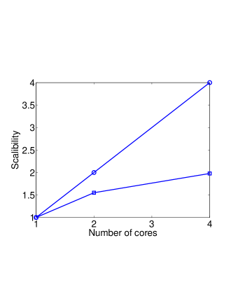
Figure 2: Scalability curve for the construction of MSCN for a $32\times 32$ grid leaky lid driven cavity problem on four cores using parallel computing toolbox of Matlab 7.10

5 Numerical experiments

The numerical experiments were performed on Matlab 7.10 in double precision arithmetic with multi-threading enabled on a core i7 (720QM) Intel processor with 8 processing threads. The system had 6GB of DDR3 RAM and 6MB of L3 cache. The iterative accelerator used is restarted GMRES with subspace dimension 300. We keep the subspace dimension large to keep avoid the effects of restart. The maximum number of iterations allowed is 3000 and the stopping criteria is the decrease of relative residual below $10^{-9}$. The given coefficient matrix is scaled by dividing each row by an entry on the same row with maximum absolute value. For the sake of comparison with sequential PCD and LSC methods, the experiments with the new methods are also done sequentially. The test set consists of standard leaky lid driven cavity problem defined on both uniform and stretched grid. The discretization scheme used is the Q2-Q1 (biquadratic velocity/bilinear pressure) mixed finite element discretization with viscosity varying from 0.1 to 0.001. A sample of the discretization of Q2-Q1 scheme for $h=1/64$ for stretched grid with stretch factor of 1.056 with more finer discretization near the boundaries is shown in figure (3).

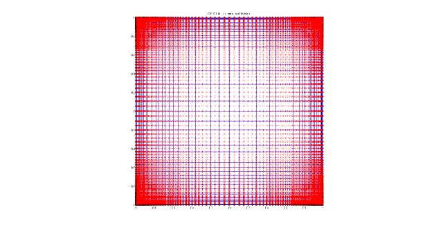
Figure 3: Q2-Q1 discretization for leaky lid driven cavity for h=1/128 stretched grid (stretch factor=1.056) with Reynolds number of 1000

These problems are generated using the IFISS software [11]. We compare all three important aspects of the methods, namely, the storage requirements, i.e., the fill factor, the iteration count, and the CPU time. For MSCE method, the parameters $p_{i}$ and $r_{i}$ are taken to be equal to “sz” defined in Table (3).

Table 3: Notations used in tables of numerical experiments

Notations	Meaning
grid	Number of discretization points
sz	Size of the Mini Schur complement
nA	Number of independent blocks in the (1,1) block
nS	Number of MSCs considered
sA	Threshold size of the diagonal blocks of (1,1) block
tolA	Tolerance for the incomplete LU approx. for (1,1) block
its	Iteration count
time	time for construction and solution excludes partition time
MSCN	Mini Schur complement with numbering based aggregation
OMSCN	Overlapped mini Schur complement with numbering based aggregation
LUM	Lumped approximation
MSCE	Mini Schur complement with edge based aggregation
MPCD	Modified pressure convection diffusion
LSC	Least square commutator
NA	Not applicable
NC	Not converged
-	Test abandonned due to relatively large time

5.1 Leaky lid driven cavity

In Table (4), we present the results for the uniform grid. We compare all three important aspects of the methods proposed namely iteration count, CPU time, and fill factor which is the ratio of the non non-zeros in the preconditioner and non-zeros in the original coefficient matrix. We compare new methods with the Pressure convection diffusion and Least square commutator methods as implemented in IFISS MATLAB toolbox. In the tables, $nA$ denote the number of diagonal block in (1,1) block and $nS$ denote the number of independent Schur complement computations. We use an incomplete LU with tolerance $10^{-4}$ as an inexact solver for the (1,1) blocks. As expected the number of iterations for the PCD and LSC methods seem to be independent of the mesh size $h$. But for the new MSC based methods there is slight increase in the iteration count. This is expected for a domain decomposition based method; more the number of subdomains more the iteration count, but more the parallelism. Nevertheless, the CPU times of the new methods are better compared to both PCD and LSC with many independent blocks. For instance, for the $h=1/32$ we have 5 subdomains for the (1,1) block and 11 subdomains for the Schur complement, while for $h=1/128$, we have 12 subdomains for the (1,1) block and 31 independent Schur complement computation. On comparing the dependence of iteration count with increasing Reynolds number, we observe that iteration count increses mildy until Reynolds number is equal to 1000. We notice that the system remains in steady state untill Reynolds number of 1000 as seen in figure (4). For Reynold number larger than 1000, we expect the unsteady state with several vortices in the strealine contours as shown in figure (5); the velocity contours suggests that the motion is nearly chaotic.

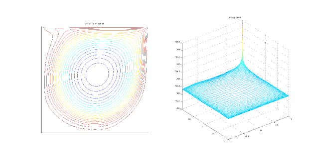
Figure 4: Left: Velocity streamlines, Right: Pressure field for leaky lid driven cavity for h=1/128 stretched grid with Q2-Q1 discretization with Reynolds number of 1000

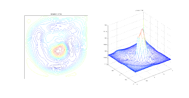
Figure 5: Left: Velocity streamlines, Right: Pressure field for leaky lid driven cavity for h=1/128 stretched grid with Q2-Q1 discretization with Reynolds number of 3000

Comparing with PCD and LSC for Reynolds number higher that 500 the iteration count for PCD and LCS are higher that the MSC based preconditioners. The size of each of the MSC are kept equal and they are equal to $sz$ in the table. The overlap for the OMSCN and OMSCNR methdods are equal to $sz$. Clearly, the overlap shows some improvements since, the approximation is better compared to the non-overlaping case. We have an interesting observation that for LUM shows same iteration count as MSCN, the reason is that the $E_{ii}$ and $F_{ii}$ blocks are very sparse and often zero and thus $G_{ii}-F_{ii}D_{ii}^{-1}E_{ii}\approx G_{ii}$. However, this is only true for the uniform grid, for stretched grid in Table (5) MSCN converges faster compared to LUM method. But all in all for both the grid OMSCN and OMSCNR seems to have less iteration count and less CPU time compared to the PCD and LSC methods. For MSCE method the convergence time was found to be very large compared to all the methods and it will be investigated in future work.

Table 4: Preconditioned GMRES on steady Oseen problems, leaky lid driven cavity, (Q2-Q1 FEM, uniform grids), for MSCN, LUM, MSCE, OMSCN, OMSCNR, MPCD, and LSC

Re	$\frac{1}{h}$	sz	nA	nS	sA	MSCN			LUM			MSCE			OMSCN			OMSCNR			MPCD		LSC
						its	tm	ff	its	tm	ff	its	tm	ff	its	tm	ff	its	tm	ff	its	tm	its	tm
	32	38	5	11	400	64	0.9	3.1	64	0.9	3.1	-	-	-	52	0.7	3.1	52	0.7	3.1	24	1.7	13	0.9
10	64	69	10	16	800	101	8	4.6	101	8	4.6	-	-	-	57	4.8	4.6	52	4.3	4.6	25	7.8	17	4.5
	128	107	12	31	2700	141	63	6.9	141	63	6.9	-	-	-	104	50	7.0	94	44	7.0	25	31	21	26
	32	38	5	11	400	66	0.9	3.5	66	0.9	3.5	-	-	-	53	0.7	3.5	53	0.7	3.5	46	2.6	31	2.2
100	64	69	10	16	800	103	7.0	4.1	103	7.0	4.1	-	-	-	61	4.2	4.1	61	4.2	4.1	48	12.5	35	9.1
	128	107	12	31	2700	165	66	6.1	165	66	6.1	-	-	-	118	46	6.2	116	45	6.2	49	55	49	56
	32	38	5	11	400	80	1.2	4.2	80	1.1	4.2	-	-	-	66	10.4	4.2	66	10.5	4.2	120	8.8	96	5.5
500	64	69	10	16	800	106	9.1	5.8	106	9.1	5.8	-	-	-	64	5.7	5.9	67	5.9	5.9	117	28.4	101	26.9
	128	107	12	31	2700	161	86	8.7	161	83	8.7	-	-	-	108	58	8.8	108	58	8.8	108	119	100	121
	32	38	5	11	400	96	1.4	4.1	96	1.4	4.1	-	-	-	83	1.2	4.2	83	1.2	4.2	179	10.5	155	9.0
1000	64	69	10	16	800	136	11	6.1	136	11	6.1	-	-	-	82	7.4	6.2	91	8.1	6.2	213	53.2	191	52.1
	128	107	12	31	2700	141	63	6.9	141	66	6.9	-	-	-	104	49	7.0	94	44	7.0	198	225	187	231
	32	38	5	11	400	253	5.1	4.7	253	5.1	4.7	-	-	-	232	4.6	4.8	232	4.6	4.8	302	18.5	300	18.6
3000	64	69	10	16	800	281	31	6.9	281	32	6.9	-	-	-	183	19	7.0	183	19	7.0	1127	362.3	1103	381.8
	128	107	12	31	2700	984	900	11.4	984	900	11.4	-	-	-	854	705	11.4	847	761	11.4	NC	NC	NC	NC

Table 5: Preconditioned GMRES on steady Oseen problems, leaky lid driven cavity, (Q2-Q1 FEM, stretched grids), for MSCN, LUM, MSCE, OMSCN, OMSCNR, MPCD, and LSC

Re	$\frac{1}{h}$	sz	nA	nS	sA	MSCN			LUM			MSCE			OMSCN			OMSCNR			MPCD		LSC
						its	tm	ff	its	time	ff	its	tm	ff	its	tm	ff	its	tm	ff	its	tm	its	tm
	32	25	5	17	400	74	0.9	3.0	74	0.9	3.0	-	-	-	46	0.6	3.0	46	0.6	3.0	23	1.3	10	1.0
10	64	101	9	11	900	65	4.7	4.1	86	6.3	4.1	-	-	-	49	3.7	4.1	48	3.6	4.1	23	8.0	28	9.2
	128	238	12	14	2700	121	51	6.1	113	47	6.1	-	-	-	79	35	6.2	85	38	6.2	23	29	40	49.2
	32	25	5	17	400	80	1.1	3.2	80	1.1	3.2	-	-	-	53	0.7	3.3	53	0.7	3.3	47	3.3	41	2.3
100	64	101	9	11	900	64	4.2	3.8	87	5.7	3.8	-	-	-	49	3.3	3.9	49	3.3	3.8	47	13.7	62	15.9
	128	238	12	14	2700	120	46	5.5	142	58	5.5	-	-	-	99	39	5.6	101	40	5.6	48	60	92	117
	32	25	5	17	400	107	1.6	4.2	107	1.6	4.2	-	-	-	86	8.8	4.3	86	8.8	4.3	160	11.1	99	7.1
500	64	101	9	11	900	65	5.2	5.1	93	7.3	6.1	-	-	-	46	4.0	5.2	48	4.1	5.2	128	34.4	143	37.6
	128	238	12	14	2700	128	55	6.9	170	78	6.9	-	-	-	106	47	7.0	114	51	7.0	133	164	193	235
	32	25	5	17	400	120	1.9	4.2	120	1.9	4.2	-	-	-	95	1.4	4.3	95	1.5	4.3	251	15.2	153	11.3
1000	64	101	9	11	900	78	6.5	5.5	111	9.3	5.5	-	-	-	59	5.2	5.6	59	5.2	5.6	248	69.3	229	61.3
	128	238	12	14	2700	133	65	7.9	176	88	7.9	-	-	-	115	56	8.0	119	58	7.9	286	364	318	393
	32	25	5	17	400	225	4.6	4.8	225	4.6	4.8	-	-	-	175	3.3	4.9	175	3.4	4.9	297	18.6	299	19.6
3000	64	101	9	11	900	240	23	6.2	284	29	6.2	-	-	-	216	21.4	6.3	226	22.2	6.3	940	316	766	240
	128	238	12	14	2700	184	101	9.3	232	130	9.3	-	-	-	163	90	9.4	165	91	9.4	1513	2228	1232	1726

6 Conclusions

In this work, we proposed a new class of algebraic approximation to the Schur complement based preconditioners for Navier-Stokes problem, we observe the superiority of the methods compared to PCD and LSC method especially for Reynolds number larger than 100. The proposed methods are highly parallel, and very suitable for modern day multiprocessor and/or multi-core systems.

As a future work, an implementation of the methods in parallel may be done and an extensive comparison with other existing preconditioners for the Navier-Stokes systems will be added. A coarse grid corrections may be introduced which may improve the convergence of the methods significantly, however, it may very well be the bottleneck in achieving overall parallelism in the two level methods.

7 Acknowledgements

I am pleased to acknowledge the generous support of Institute Henri Poincare, Paris and Université libre de Bruxelles for usual office facilities, access to library, and encouraging environment that helped in completing this work.

References

- [1] J.I. Aliaga, M. Bollhofer, A. MArtin, and E. Quintana-Orti, ILUPACK, Invited book chapter in Springer Encyclopedia of parallel computing, David Padua (ed.), Springer, to appear, ISBN: 978-0-387-09765-7.
- [2] T. Banachiewicz, Zur Berechnung der Determinanten, wie auch der Inversen, und zur darauf basierten Auflosung der systeme linearer Gleichungen, Acta Astronomica, Série C, 3, 1937, 41-67.
- [3] M. Benzi, M.K. Ng, Q. Niu, and Z. Wang, A Relaxed Dimensional Factorization Preconditioner for the Incompressible Navier-Stokes Equations, U. Minnesota, Math/CS Technical Report TR-2010-010, May 2010.
- [4] M. Benzi and X.P. Guo, A Dimensional Split Preconditioner for Stokes and Linearized Navier-Stokes Equations, Applied numerical mathematics, 61(2011), pp. 66-76.
- [5] M. Benzi, M.A. Olshanskii, and Z. Wang, Modified augumented Lagrangian preconditioners for the incompressible Navier-Stokes equations, International journal for numerical methods in fluids, March 2010.
- [6] M. Benzi, G. H. Golub, and J. Liesen, Numerical solution of Saddle Point Problems, Acta Numerica, 14 (2005), pp. 1-137.
- [7] M. Benzi and A. M. Tuma, A comparative study of sparse approximate inverse preconditioners, Applied Numerical Mathematics 30 (1999) 305-340.
- [8] D. Braess, Towards algebraic multigrid for elliptic problems of second order, Computing 55(4) (1995) 379-393.
- [9] P. Concus, G. H. Golub, and G. Meurant, Block Preconditioning for the Conjugate Gradient method, SIAM J. Sci. Statist. Comput., 6, (1985), pp.220-252
- [10] T. Davis, Direct methods for sparse linear systems, SIAM, Philadelphia, 2006.
- [11] H.C. Elman, D.J. Silvester, and A.J. Wathen, Finite elements and fast iterative solvers with applications in incompressible fluid dynamics, Oxford university press, 2005.
- [12] H.C. Elman, V.E. Howle, J. Shadid, and R. Shuttleworth, R. Tuminaro, Block preconditioners based on approximate commutators, SIAM Journal on Scientific computing 27 (2006) 1651-1668.
- [13] H.C. Elman, Preconditioning for steady state Navier-Stokes equations with low viscosity, SIAM Journal on Scientific Computing 20 (1999) 1299-1316.
- [14] H.C. Elman, D.J. Silvester, and A.J. Wathen, Performance and analysis of saddle point preconditioners for the steady state Navier-Stokes equations, Numerische Mathematik 90 (2002) 665-668.
- [15] L. Grigori, P. Kumar, F. Nataf, and K. Wang, A class of multilevel parallel preconditioning strategies \urlhttp://hal.archives-ouvertes.fr/inria-00524110/fr/
- [16] M. J. Gander, L. Halpern, and F. Nataf, Optimized Schwarz methods, International conference on domain decomposition methods, 2001.
- [17] G. Karypis and V. Kumar, A fast and high quality multilevel scheme for partitioning irregular graphs, SIAM J. Sci. Comp., (1999), 359-392.
- [18] D. Kay, D. Loghin, and A.J. Wathen, A preconditioner for the steady state Navier-Stokes equations, SIAM Journal on Scientific Computing 24 (2002) 237-256.
- [19] P. L. Lions, On the Schwarz alternating method. III: a variant for non-overlapping subdomains, In T. F. Chan, R. Glowinski, J. Périaux, O. Widlund, editors, Third International Symposium on Domain Decomposition Methods for Partial Differential Equations, held in Houston, Texas, March 20-22, 1989, Philadelphia, PA, 1990. SIAM.
- [20] P. Chevalier and F. Nataf Symmetrized method with optimized second-order conditions for the Helmholtz equation, Contemp. Math. 218, (1998) 400-407.
- [21] F. Nataf, F. Rogier, and E. de Sturler, Optimal interface conditions for domain decomposition methods , CMAP Ecole polytechnique, 1994.
- [22] F. Nataf, H. Xiang, and V. Dolean, A Coarse Space Construction Based on Local DtN Maps, 2010, \urlhttp://hal.archives-ouvertes.fr/hal-00491919/fr/.
- [23] S. V. Patankar and D.A. Spalding, A calculation procedure for heat, mass and momentum transfer in three dimensional parabolic flows, International journal on heat and mass transfer 15(1972) 1787-1806.
- [24] M. Pernice and M.D. Tocci, A multigrid preconditioned Newton-Krylov method for the incompressible Navier-Stokes eqations, SIAM Journal on Scientific Computing 123 (2001) 398-418.
- [25] J.B. Perot, An analysis of the fractional step method, Journal of computational physics 108 (1993) 51-58.
- [26] S.V. Patankar, Numerical Heat Transfer and Fluid Flow, Hemisphere Publishing Corporation, New York, 1980.
- [27] F. X. Roux, F. Magoulès, S. Samon, and L. Series, Optimization of interface operator based on algebraic approach , in 14th International conference on Domain decomposition methods in Cocoyoc, Mexico, (2002), 297-304.
- [28] F.-X. Roux, F. Magoulès, L. Series, and Y. Boubendir, Algebraic approximation of Dirichlet-to-Neumann maps for the equations of linear elasticity, Comput. Methods Appl. Mech. Engrg., 195, 2006, 3742-3759
- [29] F.-X. Roux, F. Magoulès, L. Series, and Y. Boubendir, Approximation of Optimal Interface Boundary Conditions for Two-Lagrange Multiplier FETI Method, LNCS, volume 40, 2005, 283-290
- [30] J. W. Ruge and K. Stüben, Algebraic multigrid, Multigrid Methods, Frontiers of Applied Mathematics, vol. 3. SIAM Philadelphia, PA (1987) 73-130.
- [31] Y. Saad, Iterative Methods for Sparse Linear Systems, PWS publishing company, Boston, MA, 1996.
- [32] Z. Li, Y. Saad, and M. Sosonkina, pARMS: a parallel version of the algebraic recursive multilevel solver, Num. Lin. Alg. Appl., 10, (2003), 485-509.
- [33] Y. Saad and B. Suchomel, ARMS : An algebraic recursive multilevel solver for general sparse linear systems, NLAA, 9, (2002), pp.359-378.
- [34] K. Stüben, A review of algebraic multigrid, J. Comput. Appl. Math. and applied mathematics, 128(1-2) (2001) 281-309, Numerical analysis 2000, vol. VII, Partial differential equations.
- [35] U. Trottenberg, C. W. Oosterlee, and A. Schüller, Multigrid, Academic Press Inc. San Diego, CA, 2001, with contributions by Brandt A, Oswald P, and Stüben K.