The physical origin of optical flares following GRB 110205A and the nature of the outflow

Abstract

The optical emission of GRB 110205A is distinguished by two flares. In this work we examine two possible scenarios for the optical afterglow emission. In the first scenario, the first optical flare is the reverse shock emission of the main outflow and the second one is powered by the prolonged activity of central engine. We however find out that it is rather hard to interpret the late ($t>0.1$ day) afterglow data reasonably unless the GRB efficiency is very high ($\sim 0.95$). In the second scenario, the first optical flare is the low energy prompt emission and the second one is the reverse shock of the initial outflow. Within this scenario we can interpret the late afterglow emission self-consistently. The reverse shock region may be weakly magnetized and the decline of the second optical flare may be dominated by the high latitude emission, for which strong polarization evolution accompanying the quick decline is possible, as suggested by Fan et al. in 2008. Time-resolved polarimetry by RINGO2-like polarimeters will test our prediction directly.

1 Introduction

GRB 110205A was triggered and located by the Swift Burst Alert Telescope(BAT) at 02:02:41 UT and the BAT lightcurve showed activity with multiple peaks ending at 1500 seconds after the GRB trigger, with a peak count rate of 4500 counts/s (15-150 keV) at 210 seconds after the trigger. The duration of GRB 110305A is $T_{90}=257\pm 25$ seconds in the range from 15 keV to 350 keV (Beardmore et al. 2011a, Markwardt et al. 2011).

The redshift of GRB 110205A was $z=2.2$ through detecting and analyzing the optical spectrum of the host galaxy (Cenko et al. 2011). As observed by Konus-Wind, the isotropic energy is $E_{\rm iso}=(4.34\pm 0.42)\times 10^{53}$ erg, using a standard cosmology model with $H_{0}=71{\rm km~{}s^{-1}~{}Mpc^{-1}}$, $\Omega_{\rm M}=0.27$, and $\Omega_{\Lambda}=0.73$ (Gorosabel et al. 2011).

The optical observation started at 90.6 seconds after the GRB110205A trigger (Klotz et al. 2011a). Two optical flares were detected during the observation. The optical brightness increased to the first peak of ${\rm R}\sim 16.7$ about 225 seconds after the trigger. Then the flux decreased at ${\rm R}\sim 18$ about 360 seconds after the trigger (Klotz et al. 2011b). The brightness increased again, and the second peak was ${\rm R}\sim 13.7$ at about 1140 seconds after the trigger(Andreev et al. 2011). The lightcurve of the optical flares in R-band is illuminated in Fig.1. By fitting to this lightcurve a power law $F_{t}\propto t^{-\alpha}$, we find $\alpha_{\rm I}\sim 2.5$ for the decline of the first flare. And $\alpha_{\rm IIr}\sim-4$ for the rising phase of the second flare. For the second flare decline we can obtain $\alpha_{\rm IId}\sim 2.4$ until break at $t\sim 8000$ seconds, then it decayed as $F_{t}\propto t^{-1.6}$.

The XRT began observing GRB 110205A at 02:05:16.8 UT, 155.4 seconds after the BAT trigger(Beardmore et al. 2011a). The X-ray lightcurve comprises a number of flares followed by a power-law decay. The late-time lightcurve can be modelled with a power-law decay with an index of $\alpha_{\rm x}=1.63\pm 0.10$ from the time $5.1\times 10^{3}$ sec after the trigger(Beardmore et al. 2011b).

Obviously, After the break at $t\sim 8000$ seconds, the optical decay should be the forward shock emission of the afterglow, at the same decay slope with that of X-ray afterglow.

In this work we focus on the physical origin of the optical afterglow emission and pay special attention to the magnetization of the emitting region. The possible high linear polarization of the second flare will be discussed in some detail.

2 The physical origin of the optical emission of GRB110205A

The optical lightcurve of GRB 110205A is distinguished by two flares. To interpret the data we divide the observed R-band lightcurve into three segments: phase-I is the decline phase of the first flare, phase II is the the second flare up to $t\sim 8000$ s (i.e., the break time in the decline) and phase III is the late afterglow (see Fig.1).

In this section, we focus on two possible scenarios. In the first scenario, phase-I is the reverse shock emission of the main outflow, and phase-II is the optical flare powered by the prolonged activity of the central engine. In the second scenario, phase-I is the low energy tail of the prompt soft $\gamma$-ray emission, and phase-II is the reverse shock emission of the initial outflow. In both scenarios, phase-III is the regular forward shock afterglow emission.

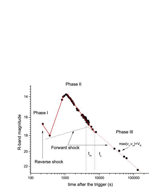
Figure 1: The interpretation of the optical emission of GRB 110205A: the first scenario. The data points are taken from Klotz et al. (2011a, 2011b), Andreev et al. (2011) and Kelemen et al. (2011).

2.1 The first scenario

The early optical emission may be powered by the reverse shock. The time when the reverse shock crosses the GRB shell can be estimated as $\rm t_{\times}{\sim max}[T_{90},t_{\rm dec}]$, where $\rm t_{\rm dec}$ is the deceleration time of the fireball and is given by $\rm t_{\rm dec}=[(3E_{\rm k}/4\pi\gamma_{0}^{2}nm_{\rm p}c^{2})^{1/3}/2\gamma_{0}^{2}c](1+z)$, where $\rm\gamma_{0}$ is the initial Lorentz factor of the GRB outflow, $n$ is the number density of the circum-burst medium, $c$ is the speed of light, $m_{\rm p}$ is the rest mass of protons and $E_{\rm k}$ is the isotropic-equivalent kinetic energy of the GRB outflow, here we assume $E_{\rm k}=5E_{\rm iso}$, corresponding to a moderate GRB efficiency $\eta_{\gamma}\equiv E_{\rm iso}/(E_{\rm iso}+E_{\rm k})\approx 0.17$. The thick shell case corresponds to $T_{90}\sim t_{\times}$ while the thin shell case corresponds to $T_{90}<t_{\times}$. For the current burst, the reverse shock emission peaks at $\rm t_{\rm p,r}=225$ sec, where the superscript ’r’ represents the parameter of the reverse shock, hence we have $t_{\times}\sim t_{\rm p,r}\sim T_{90}\sim t_{\rm dec}$ and $\gamma_{0}\sim[\frac{24E_{\rm k}(1+z)^{3}}{\pi nm_{\rm p}c^{5}t_{\rm p,r}^{3}}]^{1/8}=4.3\times 10^{2}E_{\rm k,54.3}^{1/8}n_{0}^{-1/8}t_{\rm p,r,2.4}^{-3/8}(\frac{1+z}{3.2})^{3/8}$.

When reverse shock crosses the thick shell its emission is governed by Sari & Piran (1999) and Kobayashi (2000)

$$\nu_{\rm m}^{\rm r}(t_{\times})\approx 5.0\times 10^{13}{\epsilon_{\rm e,-1}^{\rm r}}^{2}{\epsilon_{\rm B,-2}^{\rm r}}^{1/2}n_{0}^{1/2}\gamma_{0,2.6}^{2}(\frac{1+z}{3.2})^{-1}~{}{\rm Hz},$$ (1)

$$\nu_{\rm c}^{\rm r}(t_{\times})\approx 8.5\times 10^{14}{\epsilon_{\rm B,-2}^{\rm r}}^{-3/2}E_{\rm k,54.3}^{-1/2}n_{0}^{-1}(\frac{1+z}{3.2})^{-1/2}t_{\times,2.4}^{-1/2}~{}{\rm Hz},$$ (2)

$$F_{\nu,\rm max}^{\rm r}(t_{\times})\approx 5.1\times 10^{2}{\epsilon_{\rm B,-2}^{\rm r}}^{1/2}E_{\rm k,54.3}^{5/4}n_{0}^{1/4}\gamma_{0,2.6}^{-1}t_{\times,2.4}^{-3/4}(\frac{1+z}{3.2})D_{\rm L,28.7}^{-2}~{}{\rm mJy},$$ (3)

where $\epsilon_{\rm B}$ and $\epsilon_{\rm e}$ are the fractions of the shock energy given to the magnetic field and electrons at the shock front respectively, and $D_{\rm L}$ is the luminosity distance. The synchrotron emission for $\nu_{\rm m}^{\rm r}<\nu_{\rm R}<\nu_{\rm c}^{\rm r}$ is estimated by $F_{\nu_{\rm R}}^{\rm r}=F_{\nu,\rm max}^{r}(\nu_{\rm R}/\nu_{\rm m}^{\rm r})^{\rm-(p-1)/2}\approx 50{\epsilon_{\rm B,-2}^{\rm r}}{\epsilon_{\rm e,-1}^{\rm r}}^{2}E_{\rm k,54.3}^{5/4}n_{0}^{3/4}\gamma_{0,2.6}t_{\times,2.4}^{-3/4}D_{\rm L,28.7}^{-2}$ mJy, where $p$ is the power-law index of electrons distribution (i.e., $N_{\rm\gamma}\propto\gamma^{-p}$). For $t>t_{\times}$, the reverse shock emission drops with time as $F_{\nu}^{\rm r}\propto t^{\rm-(73p+21)/96}$ (Kobayashi 2000, Fan et al. 2002). Taking $p=3$, we can get $\rm F_{\nu}^{r}\propto t^{-2.5}$, matching the decline of the first flare. The reverse shock optical emission flux can be consistent with the observation for proper parameters, such as $\epsilon_{\rm e}^{\rm r}\sim 0.1$, $\epsilon_{\rm B,-2}^{\rm r}\sim 0.1$ and $n_{0}\sim 10^{-2}$.

It is however important to check whether the late ($t>0.1$ day) afterglow emission can be interpreted as the forward shock emission. For $t>0.1$ day, the X-ray and optical afterglow data decline with the time as $t^{-1.6}$, suggesting that the R-band is above both the typical synchrotron radiation frequency ($\nu_{\rm m}$) and the cooling frequency ($\nu_{\rm c}$) of the forward shock electrons. Therefore both $\nu_{c}$ and $\nu_{m}$ should cross the observer’s frequency ($\nu_{\rm R}$) before $t<0.1$ day. These two times are denoted as $t_{\rm c}$ and $t_{\rm m}$, respectively.

For the ISM-like medium and $t>t_{\rm dec}$, we have $\rm F_{\nu,max}\propto t^{0}$, $\rm\nu_{m}\propto t^{-3/2}$ and $\rm\nu_{c}\propto t^{-1/2}$ (Sari & Piran 1999). In the fast cooling case, the forward shock emission can be estimated as

$$\rm F_{\nu}=\cases{(\nu/\nu_{c})^{1/3}F_{\nu,max}\propto t^{1/6},&$\rm\nu_{m}>\nu_{c}>\nu$,\cr(\nu/\nu_{c})^{-1/2}F_{\nu,max}\propto t^{-1/4},&$\nu_{m}>\nu>\nu_{c}$,\cr(\nu_{m}/\nu_{c})^{-1/2}(\nu/\nu_{m})^{-p/2}F_{\nu,max}\propto t^{-3/2},&$\nu>\nu_{m}>\nu_{c}$,\cr}$$ (4)

where $p\sim 2.6$ has been adopted . Evidently, the forward shock R-band emission should be dimmer than $18^{\rm th}$ mag at $t=350$ s and then be the same as that detected at $t>0.1$ day. It is straightforward to show that it is not possible to find proper $t_{\rm c}$ and $t_{\rm m}$ with the scaling laws of eq.(4). Hence this possibility has been ruled out.

In the slow cooling case,

$$\rm F_{\nu}=\cases{(\nu/\nu_{m})^{1/3}F_{\nu,max}\propto t^{1/2},&$\nu_{c}>\nu_{m}>\nu$,\cr(\nu/\nu_{m})^{-(p-1)/2}F_{\nu,max}\propto t^{-6/5},&$\nu_{c}>\nu>\nu_{m}$,\cr\left(\nu_{c}/\nu_{m}\right)^{-(p-1)/2}\left(\nu/\nu_{c}\right)^{-p/2}F_{\nu,max}\propto t^{-3/2},&$\nu>\nu_{c}>\nu_{m}$.\cr}$$ (5)

In this case one can find proper $t_{\rm c}\sim 4\times 10^{3}$ s and $t_{\rm m}\sim 8\times 10^{3}$ s, as illustrated in Fig.1. Hence it deserves a further investigation. For $t>t_{\rm dec}$, the dynamics of the forward shock can be well approximated by the Blandford-McKee similar solution (Blandford & McKee 1976), which emission can be estimated by

$$F_{\nu,{\rm max}}=23~{}{\rm mJy}~{}({1+z\over 3.2})D_{\rm L,28.7}^{-2}\epsilon_{\rm B,-2}^{1/2}E_{\rm k,54.3}n_{0}^{1/2},$$ (6)

$$\nu_{\rm m}=9.0\times 10^{15}~{}{\rm Hz}~{}E_{\rm k,54.3}^{1/2}\epsilon_{\rm B,-2}^{1/2}\epsilon_{e,-1}^{2}({C_{\rm p}\over 1.6})^{2}({1+z\over 3.2})^{1/2}t_{3}^{-3/2},$$ (7)

$$\nu_{\rm c}=2.3\times 10^{15}~{}{\rm Hz}~{}E_{\rm k,54.3}^{-1/2}\epsilon_{\rm B,-2}^{-3/2}n_{0}^{-1}({1+z\over 3.2})^{-1/2}t_{3}^{-1/2},$$ (8)

where $C_{p}\equiv 13(p-2)/[3(p-1)]$. As shown in Fig.1, the data suggest that $F_{\nu,{\rm max}}\sim 0.4~{}{\rm mJy}$ i.e., $\epsilon_{\rm B,-2}^{1/2}E_{\rm k,54.3}n_{0}^{1/2}\sim 1/60$. The fact that $\nu_{\rm m}$ and $\nu_{\rm c}$ crosses $\nu_{\rm R}$ at $t_{\rm m}$ and $t_{\rm c}$ gives that $E_{\rm k,54.3}^{1/2}\epsilon_{\rm B,-2}^{1/2}\epsilon_{e,-1}^{2}\sim 0.5$ and $E_{\rm k,54.3}^{-1/2}\epsilon_{\rm B,-2}^{-3/2}n_{0}^{-1}\sim 0.6$. To reproduce the data, one needs $\epsilon_{\rm B,-2}\sim 4\times 10^{7}E_{\rm k,54.3}^{3}$, which is hard to satisfy for reasonable GRB efficiency. Let’s check whether the inverse compton effect can change the result or not. With such an effect, $\nu_{\rm c}\propto(1+Y)^{-2}$, where $Y$ is the compton parameter and can be estimated by $Y\sim(-1+\sqrt{1+4\eta\epsilon_{\rm e}/\epsilon_{\rm B}})/2$, where $\eta\sim\rm min\{1,[\nu_{\rm m}/(1+Y)^{2}\nu_{\rm c}]^{(p-2)/2}\}$. For $t\sim t_{\rm c}\sim t_{\rm m}$, we have $\nu_{\rm c}\sim\nu_{\rm m}$, $\eta\sim(1+Y)^{2-p}$ and $Y\sim(\epsilon_{\rm e}/\epsilon_{\rm B})^{0.4}$ if $\eta\epsilon_{\rm e}/\epsilon_{\rm B}\gg 1$. So the cooling frequency is estimated by $\nu_{\rm c}=3.6\times 10^{14}~{}{\rm Hz}~{}E_{\rm k,54.3}^{-1/2}\epsilon_{\rm e,-1}^{-0.8}\epsilon_{\rm B,-2}^{-0.7}n_{0}^{-1}({1+z\over 3.2})^{-1/2}t_{3}^{-1/2}$ (for $t_{\rm c}\sim 8\times 10^{3}$ s we have $E_{\rm k,54.3}^{-1/2}\epsilon_{\rm e,-1}^{-0.8}\epsilon_{\rm B,-2}^{-0.7}n_{0}^{-1}\sim 4$). In this case we need $\epsilon_{\rm B}\sim 6\times 10^{-9}E_{\rm k,54.3}^{-3.4}$ to reproduce the data, which seems too small to be reasonable. A reasonable $\epsilon_{\rm B}\sim 10^{-3}-10^{-2}$ is obtainable if we take $E_{\rm k}\sim E_{\rm iso}/20$, i.e., the GRB efficiency is as high as $\eta_{\gamma}\sim 0.95$. It is unclear how such a high GRB efficiency can be achieved. Indeed very high $\eta_{\gamma}$ have been reported for some Swift GRBs in the literature (e.g., Zhang et al. 2007; Cenko et al. 2010). One, however, should take these preliminary results with caution. For example, in the energy injection model for the X-ray shallow decline phase, a very high $\eta_{\gamma}$ can be obtained if one estimates $E_{\rm k}$ with the shallow decline data. However, as pointed out by Fan & Piran (2006) for the first time, in many cases the energy injection model can not interpret the simultaneous optical data self-consistently. Therefore the very high GRB efficiency found in the specific energy injection model is questionable. For some bursts, for instance GRB 080319B, the prompt gamma-ray emission plausibly came from a narrow energetic core while the late time afterglow emission was powered by a wider but much less powerful ejecta (e.g., Racusin et al. 2008). The derived GRB efficiency would be unreasonably high if one estimates $E_{\rm k}$ with the late afterglow data rather than the early afterglow data. Considering these uncertainties, we do not examine the ultra-high $\eta_{\gamma}$ model further.

Since neither the slow nor the fast cooling case can provide a self-consistent interpretation of the forward shock emission, we conclude that the first scenario is not favored.

2.2 The second scenario

BAT observation showed that the prompt soft gamma-ray emission with multiple peaks lasted to $>300$ seconds after the trigger. That means when the first optical flare peaked at about 225 seconds, the prompt gamma-ray emission was still ongoing. So it is possible that phase-I is the low energy tail of prompt emission. Indeed bright prompt optical emission has been well detected in some GRBs, such as GRB 041219A (Blake et al. 2005) and GRB 080319B (Racusin et al. 2008). In this case phase-II may be powered by the reverse shock of the initial prompt GRB. If correct, the fireball is thin since the reverse shock crossed the outflow at a time $t_{\times}\sim 1140~{}{\rm s}\gg T_{\rm 90}$. The initial Lorentz factor of the GRB outflow can be estimated

$$\gamma_{0}\sim[\frac{24E_{\rm k}(1+z)^{3}}{\pi nm_{\rm p}c^{5}t_{\rm\times}^{3}}]^{1/8}=2.8\times 10^{2}E_{\rm k,54.3}^{1/8}n_{0}^{-1/8}t_{\times,3.1}^{-3/8}(\frac{1+z}{3.2})^{3/8}.$$ (9)

In the thin shell case, for $\nu_{\rm m}^{\rm r}<\nu_{\rm R}<\nu_{\rm c}^{\rm r}$ and $t<t_{\times}$, $F_{\nu_{\rm R}}^{\rm r}\propto t^{2p-1}\propto t^{4.2}$ (e.g., Fan et al. 2002), consistent with the rise behavior of phase-II $F_{\nu_{\rm R}}\propto t^{4}$. The decline of phase-II is expected to be $F_{\nu_{\rm R}}\propto t^{-(27p+5)/35}$ if it is dominated by the synchrotron radiation of the cooling reverse shock electrons or alternatively $F_{\nu_{\rm R}}\propto t^{-[2+(p-1)/2]}$ if dominated by the high latitude emission of the reverse shock, in agreement with the observation for $p\sim 2.6$ (we’ll return to this point later). Therefore both the increase and the decline of phase-II can be reasonably interpreted within the reverse shock model.

Following Fan et al. (2002), the peak optical emission of reverse shock can be estimated as

$$F_{\nu_{\rm R}}^{\rm r}\approx 3~{}{\rm mJy}~{}[8(p-2)/3(p-1)]^{p-1}{\epsilon_{\rm e,-1}^{\rm r}}^{p-1}{\epsilon_{\rm B,-3}^{\rm r}}^{(p+1)/4}n_{0}^{(p+1)/4}(\gamma_{0}/280)^{p+1},$$ (10)

where the total number of the reverse-shock-accelerated electrons $\sim E_{\rm k}/\gamma_{0}m_{\rm p}c^{2}$ and the strength of reverse shock $\Gamma_{\rm rs}\sim 1.3$ have been adopted. For proper parameters, for example $\epsilon_{\rm B}^{\rm r}\sim\epsilon_{\rm e}^{\rm r}\sim 0.1$ and $n_{0}\sim 1$, the reverse shock emission is so bright that can account for the observation data.

As in the first scenario, it is important to check whether the forward shock emission can account for the late afterglow data. In principle there could be three regimes.

Case I: $\nu_{\rm R}>\rm max\{\nu_{\rm m}(t_{\times}),\nu_{\rm c}(t_{\times})\}$, for which the temporal behaviors of the forward shock optical emission are given by (e.g., Xue et al. 2009)

$$F_{\nu_{\rm R}}\propto\cases{t^{2},&for~{}~{}~{}$t<t_{\times}$,\cr t^{-1.5},&for~{}~{}~{}$t>t_{\times}$.}$$ (11)

Case II: $\nu_{\rm m}(t_{\times})<\nu_{\rm R}<\nu_{\rm c}(t_{\times})$. In this case $t_{\rm c}=2.1\times 10^{4}\rm sec~{}E_{\rm k,54.3}^{-1}\epsilon_{\rm B,-2}^{-3}n_{0}^{-2}({1+z\over 3.2})^{-1}$, at which $\nu_{\rm c}$ crosses the observer’s frequency, should be introduced. The temporal behaviors of the forward shock optical emission are given by (e.g., Xue et al. 2009)

$$F_{\nu_{\rm R}}\propto\cases{t^{3},&for~{}~{}~{}$t<t_{\times}$,\cr t^{-1.2},&for~{}~{}~{}$t_{\times}<t<t_{\rm c}$,\cr t^{-1.5},&for~{}~{}~{}$t>t_{\rm c}$.}$$ (12)

Case III: $\nu_{\rm c}(t_{\times})<\nu_{\rm R}<\nu_{\rm m}(t_{\times})$. In this case we introduce $t_{\rm m}=6.8\times 10^{3}~{}{\rm sec}~{}E_{\rm k,54.3}^{1/3}\epsilon_{\rm B,-2}^{1/3}\epsilon_{\rm e,-1}^{4/3}({1+z\over 3.2})^{1/3}$ when $\nu_{\rm m}$ crosses the observer’s frequency. The temporal behaviors of the forward shock optical emission are given by (e.g., Xue et al. 2009)

$$F_{\nu_{\rm R}}\propto\cases{t^{2},&for~{}~{}~{}$t<t_{\times}$,\cr t^{-1/4},&for~{}~{}~{}$t_{\times}<t<t_{\rm m}$,\cr t^{-1.5},&for~{}~{}~{}$t>t_{\rm m}$.}$$ (13)

Since the forward shock optical emission should be dimmer than $\sim 18^{\rm th}$ mag at $t\sim 350$ s and should be consistent with the afterglow data for $t>0.1$ day. With the temporal behaviors suggested in Case-I, the predicted optical emission at $t\sim 350$ s is much brighter than $\sim 18^{\rm th}$ mag, rending this possibility unlikely.

Usually the cooling frequency of the forward shock emission is comparable to or larger than than that of the reverse shock. In the modeling of the temporal behaviors of phase-II, the cooling frequency of the reverse shock is required to be above $\nu_{\rm R}$. Therefore Case-III is disfavored and just Case-II remains. As shown in Fig.2, Case-II works as long as $t_{\rm c}\leq 8\times 10^{3}$ s. After the reverse shock crossed the ejecta, the cooling frequency of the reverse shock electrons drops with time as $t^{-3/2}$ (Sari & Piran 1999). Therefore $\nu_{\rm c}^{r}(t_{\times})\geq(t_{\rm c}/t_{\times})^{3/2}\nu_{\rm R}$ is needed if the quickly decaying optical emission is the synchrotron radiation of the cooling reverse shock electrons (hereafter the synchrotron radiation case). Alternatively $\nu_{\rm c}^{r}(t_{\times})\geq(t_{\rm c}/t_{\times})\nu_{\rm R}$ is needed if the quickly decaying optical emission is dominated by the high latitude emission of the reverse shock (hereafter the high latitude emission case). However, we have $\nu_{\rm c}(t_{\times})\approx(t_{\rm c}/t_{\times})^{1/2}\nu_{\rm R}$. Therefore we need $\nu_{\rm c}^{r}(t_{\times})\sim(t_{\rm c}/t_{\times})\nu_{\rm c}(t_{\times})$ or $\nu_{\rm c}^{r}(t_{\times})\sim(t_{\rm c}/t_{\times})^{1/2}\nu_{\rm c}(t_{\times})$. Following Jin & Fan (2007) we have $\nu_{\rm c}^{r}(t_{\times})\sim\Re_{\rm B}^{-3}(\frac{1+Y}{1+Y^{\rm r}})^{2}\nu_{\rm c}(t_{\times})$, where $Y^{\rm r}>0$ is the Compton parameter of the reverse shock. Note that $\nu_{\rm m}^{\rm r}\sim 3\times 10^{11}~{}{\rm Hz}~{}{\epsilon_{\rm e,-1}^{\rm r}}^{2}{\epsilon_{\rm B,-2}^{\rm r}}^{1/2}n_{0}^{1/2}\ll\nu_{\rm c}^{\rm r}$ unless ${\epsilon_{\rm e,-1}^{\rm r}}\equiv{\Re_{\rm e}\epsilon_{\rm e,-1}}\sim 10$ (Fan et al. 2002), therefore $Y^{\rm r}\leq 1$ for $(\nu_{\rm m}^{\rm r}/\nu_{\rm c}^{\rm r})^{(2-p)/2}(\epsilon_{\rm e}^{\rm r}/\epsilon_{\rm B}^{\rm r})\leq 1$. Hence we have $\nu_{\rm c}^{r}(t_{\times})\sim\Re_{\rm B}^{-3}(1+Y)^{2}\nu_{\rm c}(t_{\times})$, which further gives that ${\Re_{\rm B}}\sim 0.5(1+Y)^{2/3}$ (synchrotron radiation case) or ${\Re_{\rm B}}\sim 0.7(1+Y)^{2/3}$ (high latitude emission case), implying the outflow could be (weakly) magnetized for $Y\sim(\epsilon_{\rm e}/\epsilon_{\rm B})^{0.4}\geq{\rm a~{}few}$.

A magnetized outflow is also consistent with the flux analysis. In Case-II, the ratio between the reverse shock optical emission and forward shock optical emission at the crossing time of the reverse shock can be estimated by (Jin & Fan 2007; Fan et al. 2002; Zhang et al. 2003)

$$\frac{\rm F_{\nu_{\rm R}}^{r}(t_{\times})}{\rm F_{\nu_{\rm R}}(t_{\times})}\approx 0.08\Re_{\rm e}^{p-1}\Re_{\rm B}^{\frac{p+1}{2}}=0.08\Re_{\rm e}^{1.6}\Re_{\rm B}^{1.8}.$$ (14)

The current observation suggests that $F_{\nu_{\rm R}}^{r}(t_{\times})/F_{\nu_{\rm R}}(t_{\times})\geq 4$, we then have $\Re_{\rm e}^{1.6}\Re_{\rm B}^{1.8}\geq 50$, i.e.,

$$\Re_{\rm B}\geq 8.8\Re_{\rm e}^{-0.9}.$$ (15)

For $\Re_{\rm e}\leq 10$ we have $\Re_{\rm B}\geq 1$ unless phase-II was dominated by the emission of prolonged activity of the central engine (e.g., Gao 2009).

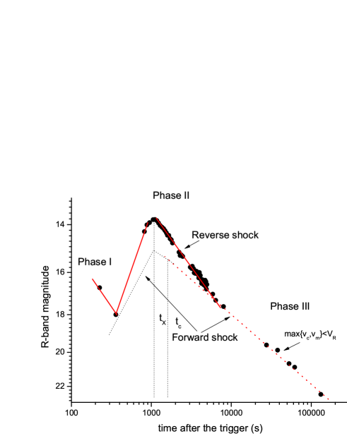
Figure 2: The interpretation of the optical emission of GRB 110205A: the second scenario.

3 The expected polarization property of the optical flares

The polarimetry of prompt emission or the reverse shock emission is very important for diagnosing the composition of the GRB outflow, since the late afterglow, taking place hours after the trigger, is powered by the external forward shock, so that essentially all the initial information about the ejecta has lost. If the GRB ejecta is initially magnetized, the prompt $\gamma-$ray/X-ray/UV/optical emission and the reverse shock emission should be linearly polarized (Lyutikov et al. 2003; Granot 2003; Fan et al. 2004). In a few events, the prompt $\gamma-$ray polarimetry are available but the results are quite uncertain. Even for the very bright GRB 041219A, a systematic effect that could mimic the weak polarization signal could not be excluded (McGlynn et al., 2007). So far, the most reliable polarimetry is that in UV/optical band (e.g., Covino et al. 1999). The optical polarimetry of the prompt emission or the reverse shock emission demands a quick response of the telescope to the GRB alert and is thus very challenging. Nevertheless, significant progress have been made since 2006. Using a ring polarimeter on the robotic Liverpool Telescope, Mundell et al. (2007) got an upper limit $\sim 8\%$ of the optical polarization of the afterglow of GRB 060418 at 203 sec after the trigger. A breakthrough was made in GRB 090102, for which Steele et al. (2009) found out that the reverse shock emission was linearly polarized with a degree $\sim 10.1\%$. The forward-reverse shock modeling of the afterglow emission suggests a mildly magnetized reverse shock region (Fan 2009; Mimica et al. 2010 ). These two findings are consistent with each other and provide the most compelling evidence so far for the magnetized outflow model for GRBs.

For the current event, we have shown that phase-I may be the low energy tail of the prompt emission and phase-II is likely the reverse shock emission though other possibility—the prolonged activity of the central engine can not be ruled out. In the reverse shock model we find out that the initial outflow could be weakly magnetized. Assuming that in the emitting region the strength ratio of the ordered magnetic field and the random magnetic field is $b$, the degree of net polarization can be roughly estimated as $\Pi_{\rm net}\approx 0.6b^{2}/(1+b^{2})$ (e.g., Fan et al. 2004). Therefore a moderate or high linear-polarization-degree of the weakly magnetized reverse shock emission is possible. In reality the configuration of the outflowing magnetic field may be very complicated and the direction of the lines may be not well ordered, for which the net polarization degree should be lowered. In section 2.2 we have shown that the decline of the second optical flare may be dominated by the high latitude emission of the reverse shock. In such a case, an interesting polarization degree evolution presents if at late times (i.e., $t>t_{\times}$) the edge of the ejecta is visible (see Fig.2 of Fan et al. 2008 for illustration). Alternatively if the decline of the second optical flare is shaped by the synchrotron radiation of the cooling reverse shock electrons, the observed linear polarization should be $\Pi=(\Pi^{r}F_{\nu_{{}_{\rm R}}}^{r}+\Pi F_{\nu_{{}_{\rm R}}})/(F_{\nu_{{}_{\rm R}}}^{r}+F_{\nu_{{}_{\rm R}}})$, where $\Pi\sim 1.4\%$ ($\Pi^{r}$) is the linear polarization of the forward (reverse) shock emission (Gorosabel et al. 2011), and $F_{\nu_{{}_{\rm R}}}$ ($F_{\nu_{{}_{\rm R}}}^{\rm r}$) is the R-band flux of the forward (reverse) shock emission. One thus expects a steady decline of the polarization degree with the time.

The Liverpool Telescope began automatically observing Swift GRB 110205A with the RINGO2 polarimeter (Mundell et al. 2011). RINGO2 is quite sensitive and can measure the linear polarization degree down to 0.9$\%$ for the source as bright as $R=17$ mag with the exposure time of 100 seconds. Therefore the linear polarization of first optical flare might be detectable if it is significantly polarized. For the second optical flare, the emission is so bright that the time-resolved polarization property can be achieved. The observations of Liverpool Telescope on GRB 110205A have stopped due to bad weather and the polarization data have not been published yet. Nevertheless the current optical data have shed some light on the nature of the GRB outflow and have suggested very interesting polarization properties.

4 Conclusion and Discussion

The Early optical emission of GRB 110205A is characterized by two flares. Two possible scenarios have been examined in this work. In the first scenario, the first optical flare is the reverse shock emission of the main outflow, the second flare is the emission powered by the prolonged activity of the central engine, and the late time ($t>0.1$ day) optical emission is the regular forward shock emission. However we find that a self-consistent interpretation of the forward shock emission is hard to achieve unless the GRB efficiency is $\sim 0.95$. Therefore this scenario is disfavored. In the second scenario, the first optical flare is the low energy prompt emission while the second flare is the reverse shock emission of the main outflow. The late optical emission is still attributed to the regular forward shock. Within this scenario a self-consistent interpretation is achieved (please note that the different Inverse Compton parameters for the reverse and forward socks play an important role in the modeling). There are two interesting findings. One is that the reverse shock region may be weakly magnetized and a moderate linear polarization degree is likely. The other is that the decline of the second optical flare may be dominated by the high latitude emission. Similar to the X-ray case, one may expect dramatic polarization evolution (Fan et al. 2008) accompanying the optical flare decline rather than the steady decrease of the polarization degree. In reality the configuration of the out-flowing magnetic field may be very complicated and the direction of the lines may be not well ordered, for which the net polarization degree should be lowered and the polarization evolution may be very complicated.

The Liverpool Telescope began automatically observing Swift GRB 110205A with the RINGO2 polarimeter (Mundell et al. 2011). RINGO2 is very sensitive. The linear polarization of first optical flare may be detectable if it is significantly polarized. For the second optical flare, the emission is so bright that the time-resolved polarization properties can be achieved. Therefore our prediction, in particular strong polarization evolution in the decline phase of the second optical flare, can be directly tested.