Intersection Theory on Mixed Curves

Abstract.

We consider two mixed curve $C,C^{\prime}\subset{\mathbb{C}}^{2}$ which are defined by mixed functions of two variables $\mbox{\bf z}=(z_{1},z_{2})$. We have shown in [4], that they have canonical orientations. If $C$ and $C^{\prime}$ are smooth and intersect transversely at $P$, the intersection number $I_{top}(C,C^{\prime};P)$ is topologically defined. We will generalize this definition to the case when the intersection is not necessarily transversal or either $C$ or $C^{\prime}$ may be singular at $P$ using the defining mixed polynomials.

1. Introduction

First we recall the complex analytic situation. Consider complex polynomials $f(\mbox{\bf z})$ and $g(\mbox{\bf z})$ of two variables $\mbox{\bf z}=(z_{1},z_{2})$ and consider complex analytic curves defined by $C:f(\mbox{\bf z})=0$ and $C^{\prime}:g(\mbox{\bf z})=0$. Suppose that $P$ is an isolated intersection point of $C\cap C^{\prime}$. Then the local algebraic intersection number $I(f,g;P)$ is defined by the dimension of the quotient module $\dim\,\mathcal{O}_{P}/(f,g)$ where $\mathcal{O}_{P}$ is the local ring of the holomorphic functions at $P$ and $(f,g)$ is the ideal generated by $f$ and $g$. Thus $I(f,g;P)$ a strictly positive integer and it is equal to 1 if and only if $C$ and $C^{\prime}$ are non-singular at $P$ and transversal each other. On the other hand, the complex curves $C,C^{\prime}$ have canonical orientations which come from their complex structures (see for example, [1]) and the local algebraic intersection number is equal to the local topological intersection number if the intersection is transverse. Moreover this is also true for non-transverse intersection in the sense that under a slight perturbation, an intersection $P$ of algebraic intersection number $\nu$ splits into $\nu$ transverse intersections. In particular, the topological local intersection number can be defined by the algebraic local intersection number.

The purpose of this note is to define the local intersection multiplicity for two mixed curves using the defining polynomials and study the analogues properties. The problem in this case is that the local intersection number is not necessarily positive. This makes the algebraic calculation more difficult. Let $C:\,f(\mbox{\bf z},\bar{}\mbox{\bf z})=0$ and $C^{\prime}:\,g(\mbox{\bf z},\bar{}\mbox{\bf z})=0$ be mixed curves which have at worst isolated mixed singularity at $P\in C\cap C^{\prime}$. We will define the intersection multiplicity $I_{top}(C,C^{\prime};P)$ using a certain mapping degree which is described by the defining polynomials $f,g$ (Definition 4, §2 and Theorem 1). This definition coincides with the usual one for complex analytic curves.

In §4, we consider the roots of a mixed polynomial $h(u,\bar{u})$ of one variable $u$ as a special case. We introduce the notion of multiplicity with sign $\rm{m_{s}}\/(f,\alpha)$ for a root $\alpha$ of $h(u,\bar{u})=0$ and we give a formulae for the description of $\rm{m_{s}}\/(f,\alpha)$ for an admissible mixed polynomial $h(u,\bar{u})$ (Theorem 17).

2. Mixed curves

2.1. A mixed singular point

Let $f(\mbox{\bf z},\bar{}\mbox{\bf z}),\,\mbox{\bf z}=(z_{1},z_{2})\in{\mathbb{C}}^{2}$, be a mixed polynomial. See [5, 4] for further details about a mixed polynomial. Using real coordinates $(x_{1},y_{1},x_{2},y_{2})$ with $z_{j}=x_{j}+iy_{j},\,j=1,2$, $f$ can be understood as a sum of two polynomials with real coefficients:

$$f(\mbox{\bf z},\bar{}\mbox{\bf z})=f_{{\mathbb{R}}}(x_{1},y_{1},x_{2},y_{2})+if_{I}(x_{1},y_{1},x_{2},y_{2}).$$

where $f_{{\mathbb{R}}},f_{I}$ are the real part and the imaginary part of $f$ respectively. Recall that $f(\mbox{\bf z},\bar{}\mbox{\bf z})$ is a polynomial of $x_{1},y_{1},x_{2},y_{2}$ by the substitution

$$z_{j}=\frac{z_{j}+\bar{z}_{j}}{2},\quad\bar{z}_{j}=\frac{z_{j}-\bar{z}_{j}}{2i},\quad j=1,2.$$

We say that $C:f(\mbox{\bf z},\bar{}\mbox{\bf z})=0$ is mixed non-singular at $P\in C$ if the Jacobian matrix of $(f_{{\mathbb{R}}},f_{I})$ has rank two at $P$ ([3, 5]). We recall that ${\mathbb{C}}^{2}$ has a canonical orientation given from the complex structure. We identify ${\mathbb{C}}^{2}$ with ${\mathbb{R}}^{4}$ by $(z_{1},z_{2})\leftrightarrow(x_{1},y_{1},x_{2},y_{2})$ and thus a positive frame of ${\mathbb{R}}^{4}$ is given by $(\frac{\partial}{\partial x_{1}},\frac{\partial}{\partial y_{1}},\frac{\partial}{\partial x_{2}},\frac{\partial}{\partial y_{2}})$. If $P$ is a mixed non-singular point, $C$ is locally a real two dimensional manifold. The normal bundle $N_{C,P}$ of $C\subset{\mathbb{C}}^{2}$ at $P$ has the canonical orientation so that the orientation is compatible with the complex valued function $f$, namely $df_{P}:N_{C,P}\to T_{0}{\mathbb{C}}$ is an orientation preserving isomorphism. Thus the orientation of $C$ at $P$ is defined as follows. A frame $(\mbox{\bf v}_{1},\mbox{\bf v}_{2})\subset T_{P}C$, $\mbox{\bf v}_{1}=(v_{11},v_{12},v_{13},v_{14}),\mbox{\bf v}_{2}=(v_{21},v_{22},v_{23},v_{24})$, is positive if and only if the frame

$$M:=\left(\begin{matrix}\bf\mbox{\bf v}_{1}\\ \bf\mbox{\bf v}_{2}\\ {{\rm{grad}\/}}\,f_{{\mathbb{R}}}\\ {{\rm{grad}\/}}\,f_{I}\end{matrix}\right)=\left(\begin{matrix}v_{11}&v_{12}&v_{13}&v_{14}\\ v_{21}&v_{22}&v_{23}&v_{24}\\ \frac{\partial f_{{\mathbb{R}}}}{\partial x_{1}}&\frac{\partial f_{{\mathbb{R}}}}{\partial y_{1}}&\frac{\partial f_{{\mathbb{R}}}}{\partial x_{2}}&\frac{\partial f_{{\mathbb{R}}}}{\partial y_{2}}\\ \frac{\partial f_{I}}{\partial x_{1}}&\frac{\partial f_{I}}{\partial y_{1}}&\frac{\partial f_{I}}{\partial x_{2}}&\frac{\partial f_{I}}{\partial y_{2}}\\ \end{matrix}\right)$$

is a positive frame of ${\mathbb{C}}^{2}={\mathbb{R}}^{4}$. The gradient vector ${{\rm{grad}\/}}\,h(x_{1},y_{1},x_{2},y_{2})$ of a real valued function $h$ is defined by

$${{\rm{grad}\/}}\,h(x_{1},y_{1},x_{2},y_{2})=(\frac{\partial h}{\partial x_{1}},\frac{\partial h}{\partial y_{1}},\frac{\partial h}{\partial x_{2}},\frac{\partial h}{\partial y_{2}}).$$

2.2. Mixed homogenization and the closure in ${\mathbb{P}}^{2}$

Assume that $f(\mbox{\bf z},\bar{}\mbox{\bf z})=\sum_{\nu,\mu}c_{\nu\mu}\mbox{\bf z}^{\nu}{\bar{}\mbox{\bf z}}^{\mu}$ is a mixed polynomial of two variables $\mbox{\bf z}=(z_{1},z_{2})$. Put $C=f^{-1}(0)\subset{\mathbb{C}}^{2}$. We assume that $C$ is non-empty and that $C$ has only finite number of mixed singular points. We consider the affine space ${\mathbb{C}}^{2}$ with coordinates z as the affine chart $Z_{0}\neq 0$ of the projective space ${\mathbb{P}}^{2}$ with homogeneous coordinates $(Z_{0},Z_{1},Z_{2})$. The coordinates are related by $z_{1}=Z_{1}/Z_{0},z_{2}=Z_{2}/Z_{0}$. Let $d^{+}$ and $d^{-}$ be the degree of $f(\mbox{\bf z},\bar{}\mbox{\bf z})$ in z and $\bar{}\mbox{\bf z}$ respectively. That is,

$$d^{+}=\max\{|\nu|\,|\,c_{\nu\mu}\neq 0\},\,\,d^{-}=\max\{|\mu|\,|\,c_{\nu\mu}\neq 0\}$$

where $|\nu|=\nu_{1}+\nu_{2}$ for a multi-integer $\nu=(\nu_{1},\nu_{2})$. We assocate with $f$ a strongly polar homogeneous mixed polynomial $F(\mbox{\bf Z},\bar{}\mbox{\bf Z})$ as follows, where $\mbox{\bf Z}=(Z_{0},Z_{1},Z_{2})$ and $\bar{}\mbox{\bf Z}=(\bar{Z}_{0},\bar{Z}_{1},\bar{Z}_{2})$ by $F(\mbox{\bf Z},\bar{}\mbox{\bf Z}):=Z_{0}^{d_{+}}{\bar{Z}_{0}}^{d^{-}}f(\frac{Z_{1}}{Z_{0}},\frac{Z_{2}}{Z_{0}},\frac{\bar{Z}_{1}}{\bar{Z}_{0}},\frac{\bar{Z}_{2}}{\bar{Z}_{0}})$ and we call $F$ the mixed homogenization of $f$. We define $\bar{C}\subset{\mathbb{P}}^{2}$ by the topological closure of $C\subset{\mathbb{C}}^{2}\subset{\mathbb{P}}^{2}$ and we defines a mixed projective curve $\tilde{C}:=\{((Z_{o}:Z_{1}:Z_{2})\in{\mathbb{P}}^{2}\,|\,F(\mbox{\bf Z},\bar{}\mbox{\bf Z})=0\}$. It is easy to see that the closure $\bar{C}$ of $C$ in ${\mathbb{P}}^{2}$ is a subset of $\tilde{C}$ but in general, $\bar{C}$ might be a proper subvariety of $\tilde{C}$. $F$ is a strongly polar homogeneous polynomial of radial degree $d^{+}+d^{-}$ and the polar degree $d^{+}-d^{-}$respectively and $F|_{Z_{0}\neq 0}=f$. In [4], we have assumed that the polar degree is non-zero for the definition of strongly polar homogeneous polynomials, but in this paper, we consider also the case $d^{+}=d^{-}$.

3. Intersection numbers

3.1. Local intersection number I (Smooth and transversal intersection case)

In this section, we denote vectors in ${\mathbb{R}}^{4}$ by column vectors for brevity’s sake. Assume that $C:f=0$ and $C^{\prime}:g=0$ are two mixed curves and assume that $P\in C\cap C^{\prime}$ and $C,C^{\prime}$ are mixed non-singular at $P$ and the intersection is transverse at $P$. Let $\mbox{\bf u}_{1},\mbox{\bf u}_{2}$ and $\mbox{\bf v}_{1},\mbox{\bf v}_{2}$ be positive frames of $T_{P}C$ and $T_{P}C^{\prime}$. Then the local (topological) intersection number $I_{top}(C,C^{\prime};P)$ is defined by the sign of the determinant $\det(\mbox{\bf u}_{1},\mbox{\bf u}_{2},\mbox{\bf v}_{1},\mbox{\bf v}_{2})$ (See for example [2]). Namely

$$I_{top}(C,C^{\prime};P)=\begin{cases}1,&\quad\det(\mbox{\bf u}_{1},\mbox{\bf u}_{2},\mbox{\bf v}_{1},\mbox{\bf v}_{2})>0,\\ -1,&\quad\det(\mbox{\bf u}_{1},\mbox{\bf u}_{2},\mbox{\bf v}_{1},\mbox{\bf v}_{2})<0.\end{cases}$$

For any frames $\mbox{\bf w}_{1},\dots,\mbox{\bf w}_{4}$ of ${\mathbb{R}}^{4}$, we define

$${\rm{Sign}}(\mbox{\bf w}_{1},\mbox{\bf w}_{2},\mbox{\bf w}_{3},\mbox{\bf w}_{4}):=\begin{cases}1,\quad&\text{if}\,\,\det(\mbox{\bf w}_{1},\mbox{\bf w}_{2},\mbox{\bf w}_{3},\mbox{\bf w}_{4})>0\\ -1,\quad&\text{if}\,\,\det(\mbox{\bf w}_{1},\mbox{\bf w}_{2},\mbox{\bf w}_{3},\mbox{\bf w}_{4})<0.\end{cases}$$

By the definition of the orientation of $C$ and $C^{\prime}$,

$$\begin{split}&{\rm{Sign}}(\mbox{\bf u}_{1},\mbox{\bf u}_{2},{{{}^{t}\rm{grad}\/}}\,f_{{\mathbb{R}}}(P),{{{}^{t}\rm{grad}\/}}\,f_{I}(P))=1,\\ &{\rm{Sign}}(\mbox{\bf v}_{1},\mbox{\bf v}_{2},{{{}^{t}\rm{grad}\/}}\,g_{{\mathbb{R}}}(P),{{{}^{t}\rm{grad}\/}}\,g_{I}(P))=1.\end{split}$$

Now our first result is the following.

Theorem 1.

The intersection number $I_{top}(C,C^{\prime};P)$ is given by

$${\rm{Sign}}({{{}^{t}\rm{grad}\/}}\,f_{{\mathbb{R}}}(P),{{{}^{t}\rm{grad}\/}}\,f_{I}(P),{{{}^{t}\rm{grad}\/}}\,g_{{\mathbb{R}}}(P),{{{}^{t}\rm{grad}\/}}\,g_{I}(P)).$$

Recall that the tangent space $T_{P}C$ is generated by the vectors orthogonal to the two dimensional subspace $<{{{}^{t}\rm{grad}\/}}\,f_{{\mathbb{R}}}(P),{{{}^{t}\rm{grad}\/}}\,f_{I}(P)>_{{\mathbb{R}}}$. Thus two dimensional planes $<\mbox{\bf u}_{1},\mbox{\bf u}_{2}>_{{\mathbb{R}}}$ and $<{{{}^{t}\rm{grad}\/}}\,f_{{\mathbb{R}}}(P),{{{}^{t}\rm{grad}\/}}\,f_{I}(P)>_{{\mathbb{R}}}$ are orthogonal. Here $<\mbox{\bf w}_{1},\mbox{\bf w}_{2}>_{{\mathbb{R}}}$ is the two dimensional plane spanned by $\mbox{\bf w}_{1},\mbox{\bf w}_{2}$.

3.1.1. Gram-Schmidt orthonormalization

First we consider a simple assertion. Let $\mbox{\bf a}_{1},\mbox{\bf a}_{2},\mbox{\bf a}_{3},\mbox{\bf a}_{4}$ be column vectors in ${\mathbb{R}}^{4}$ and let $P,Q$ be $2\times 2$ matrices. Then

Assertion 2.

$$\det((\mbox{\bf a}_{1},\mbox{\bf a}_{2})P,(\mbox{\bf a}_{3},\mbox{\bf a}_{4})Q)=\det(\mbox{\bf a}_{1},\mbox{\bf a}_{2},\mbox{\bf a}_{3},\mbox{\bf a}_{4})\det(P)\det(Q)$$

Proof.

The assertion follows from the simple equality in $4\times 4$ matirices:

$$((\mbox{\bf a}_{1},\mbox{\bf a}_{2})P,(\mbox{\bf a}_{3},\mbox{\bf a}_{4})Q)=(\mbox{\bf a}_{1},\mbox{\bf a}_{2},\mbox{\bf a}_{3},\mbox{\bf a}_{4})\left(\begin{matrix}P&O\\ O&Q\end{matrix}\right).$$

∎

Now we consider Gram-Schmidt orthnormalization of $(\mbox{\bf u}_{1},\mbox{\bf u}_{2})$ and
$({{{}^{t}\rm{grad}\/}}\,f_{{\mathbb{R}}},{{{}^{t}\rm{grad}\/}}\,f_{I})$. They are orthonormal frames $(\mbox{\bf u}_{1}^{\prime},\mbox{\bf u}_{2}^{\prime})$ and
$({{{}^{t}\rm{grad}\/}}\,f_{{\mathbb{R}}}(P)^{\prime},{{{}^{t}\rm{grad}\/}}\,f_{I}(P)^{\prime})$ such that they satisfy the equalities:

$$\begin{split}&(\mbox{\bf u}_{1}^{\prime},\mbox{\bf u}_{2}^{\prime})=(\mbox{\bf u}_{1},\mbox{\bf u}_{2})Q_{1},\,\,\text{and}\\ &({{{{}^{t}\rm{grad}\/}}}\,f_{{\mathbb{R}}}(P)^{\prime},{{{{}^{t}\rm{grad}\/}}}\,f_{I}(P)^{\prime})=({{{{}^{t}\rm{grad}\/}}}\,f_{{\mathbb{R}}}(P),{{{}^{t}\rm{grad}\/}}\,f_{I}(P))Q_{2}\end{split}$$

where $Q_{1},Q_{2}$ are upper triangular $2\times 2$ matrices with positive entries in their diagonals. Similarly we consider the orthnormalization

$$\begin{split}&(\mbox{\bf v}_{1}^{\prime},\mbox{\bf v}_{2}^{\prime})=(\mbox{\bf v}_{1},\mbox{\bf v}_{2})R_{1}\\ &({{{}^{t}\rm{grad}\/}}g_{{\mathbb{R}}}(P)^{\prime},{{{}^{t}\rm{grad}\/}}g_{I}(P)^{\prime})=({{{}^{t}\rm{grad}\/}}g_{{\mathbb{R}}}(P),{{{}^{t}\rm{grad}\/}}g_{I}(P))R_{2},\end{split}$$

where $R_{1},R_{2}$ are upper triangular matrices with with positive entries in their diagonals. Using Assertion 2, we get

$$\begin{split}{\rm{Sign}}(\mbox{\bf u}_{1}^{\prime},\mbox{\bf u}_{2}^{\prime},\mbox{\bf v}_{1}^{\prime},\mbox{\bf v}_{2}^{\prime})&={\rm{Sign}}((\mbox{\bf u}_{1},\mbox{\bf u}_{2})Q_{1},(\mbox{\bf v}_{1},\mbox{\bf v}_{2})R_{1})\\ &={\rm{Sign}}(\mbox{\bf u}_{1},\mbox{\bf u}_{2},\mbox{\bf v}_{1},\mbox{\bf v}_{2})\end{split}$$

$$\begin{split}{\rm{Sign}}&({{{}^{t}\rm{grad}\/}}f_{{\mathbb{R}}}(P)^{\prime},{{{}^{t}\rm{grad}\/}}\,f_{I}(P)^{\prime},{{{}^{t}\rm{grad}\/}}\,g_{{\mathbb{R}}}(P)^{\prime},{{{}^{t}\rm{grad}\/}}\,g_{I}(P)^{\prime})\\ &={\rm{Sign}}(({{{}^{t}\rm{grad}\/}}f_{{\mathbb{R}}}(P),{{{}^{t}\rm{grad}\/}}\,f_{I}(P))Q_{2},({{{}^{t}\rm{grad}\/}}\,g_{{\mathbb{R}}}(P),{{{}^{t}\rm{grad}\/}}\,g_{I}(P))R_{2})\\ &={\rm{Sign}}({{{}^{t}\rm{grad}\/}}f_{{\mathbb{R}}}(P),{{{}^{t}\rm{grad}\/}}\,f_{I}(P),{{{}^{t}\rm{grad}\/}}\,g_{{\mathbb{R}}}(P),{{{}^{t}\rm{grad}\/}}\,g_{I}(P)).\end{split}$$

Thus the calculation of the intersection number can be done using these orthonormal frames

$$(\mbox{\bf u}_{1}^{\prime},\mbox{\bf u}_{2}^{\prime},{{{}^{t}\rm{grad}\/}}\,f_{{\mathbb{R}}}(P)^{\prime},{{{}^{t}\rm{grad}\/}}\,f_{I}(P)^{\prime}),\,(\mbox{\bf u}_{1}^{\prime},\mbox{\bf v}_{2}^{\prime},{{{}^{t}\rm{grad}\/}}\,g_{{\mathbb{R}}}(P)^{\prime},{{{}^{t}\rm{grad}\/}}\,g_{I}(P)^{\prime}).$$

Thus the proof of Theorem 1 reduces to the following.

Lemma 3.

Assume that $(\mbox{\bf u}_{1},\mbox{\bf u}_{2},\mbox{\bf u}_{3},\mbox{\bf u}_{4})$ and $(\mbox{\bf v}_{1},\mbox{\bf v}_{2},\mbox{\bf v}_{3},\mbox{\bf v}_{4})$ be positive orthonormal frames of ${\mathbb{R}}^{4}$. Then

$$\det(\mbox{\bf u}_{1},\mbox{\bf u}_{2},\mbox{\bf v}_{1},\mbox{\bf v}_{2})=\det(\mbox{\bf u}_{3},\mbox{\bf u}_{4},\mbox{\bf v}_{3},\mbox{\bf v}_{4}).$$

Proof.

Assume that

(1) $$(\mbox{\bf u}_{1},\mbox{\bf u}_{2},\mbox{\bf u}_{3},\mbox{\bf u}_{4})=(\mbox{\bf v}_{1},\mbox{\bf v}_{2},\mbox{\bf v}_{3},\mbox{\bf v}_{4})A,$$

with $A\in SO(4;{\mathbb{R}})$. Write $A$ by $2\times 2$ matrices as

$$A=\left(\begin{matrix}A_{1}&A_{2}\\ B_{1}&B_{2}\end{matrix}\right)$$

The equality (1) can be rewritten as

(2) $$(\mbox{\bf v}_{1},\mbox{\bf v}_{2},\mbox{\bf v}_{3},\mbox{\bf v}_{4})=(\mbox{\bf u}_{1},\mbox{\bf u}_{2},\mbox{\bf u}_{3},\mbox{\bf u}_{4})\,{}^{t}A$$

where

$${}^{t}A=\left(\begin{matrix}{}^{t}A_{1}&{}^{t}B_{1}\\ {}^{t}A_{2}&{}^{t}B_{2}\end{matrix}\right).$$

First we consider the equality from (1):

$$\begin{split}\det(\mbox{\bf u}_{1},\mbox{\bf u}_{2},\mbox{\bf v}_{1},\mbox{\bf v}_{2})&=\det((\mbox{\bf v}_{1},\mbox{\bf v}_{2})A_{1}+(\mbox{\bf v}_{3},\mbox{\bf v}_{4})B_{1},\mbox{\bf v}_{1},\mbox{\bf v}_{2})\\ &=\det(\mbox{\bf v}_{1},\mbox{\bf v}_{2},(\mbox{\bf v}_{3},\mbox{\bf v}_{4})B_{1})\\ &=\det B_{1}.\end{split}$$

On the other hand, we have also from (2):

(3) $$\det(\mbox{\bf u}_{1},\mbox{\bf u}_{2},\mbox{\bf v}_{1},\mbox{\bf v}_{2}) =\det(\mbox{\bf u}_{1},\mbox{\bf u}_{2},(\mbox{\bf u}_{3},\mbox{\bf u}_{4})\,{}^{t}A_{2})$$

(4) $$=\det\,{}^{t}A_{2}=\det A_{2}$$

Thus $\det A_{2}=\det B_{1}$. Similarly we get

$$\begin{split}\det(\mbox{\bf u}_{3},\mbox{\bf u}_{4},\mbox{\bf v}_{3},\mbox{\bf v}_{4})&=\det((\mbox{\bf v}_{1},\mbox{\bf v}_{2})A_{2},\mbox{\bf v}_{3},\mbox{\bf v}_{4})=\det\,A_{2}\\ &=\det(\mbox{\bf u}_{3},\mbox{\bf u}_{4},(\mbox{\bf v}_{1},\mbox{\bf v}_{2})\,{}^{t}B_{1})=\det\,B_{1}.\\ \end{split}$$

Thus the assertion follows from these equalities. ∎

3.2. Local intersection number II (General case)

Assume that $C:\,f(\mbox{\bf z},\bar{}\mbox{\bf z})=0$ and $C^{\prime}:g(\mbox{\bf z},\bar{}\mbox{\bf z})=0$ be mixed curve as above and let $P$ be an isolated intersection point of $C\cap C^{\prime}$. We assume also that both $C$ and $C^{\prime}$ have at worst an isolated mixed singularity at $P$.

Definition 4.

Let $\varphi=(f_{{\mathbb{R}}},f_{I},g_{{\mathbb{R}}},g_{I}):{\mathbb{R}}^{4}\to{\mathbb{R}}^{4}$. We define the local intersection number $I_{top}C,C^{\prime};P)$ by the local mapping degree of the normalized mapping $\psi$ of $\varphi$:

$$\psi:=\varphi/\|\varphi\|:S_{\varepsilon}^{3}(P)\to S^{3}.$$

Here $S_{\varepsilon}^{3}(P):=\{\mbox{\bf x}\in{\mathbb{R}}^{4}\,|\,\|\mbox{\bf x}-P\|=\varepsilon\}$ and $\varepsilon$ is a sufficiently small positive number so that $P$ is the only intersection of $C$ and $C^{\prime}$ in $B_{\varepsilon}(P)$ where $B_{\varepsilon}(P)$ is the disk of radius $\varepsilon$ centered at $P$.

Suppose that $P$ is a transverse intersection of $C$ and $C^{\prime}$ and assume that $C$ and $C^{\prime}$ are mixed smooth at $P$. Take a small positive number $\varepsilon$ so that

$$\|\varphi^{(1)}(\mbox{\bf z})\|\geq 2\|\varphi-\varphi^{(1)}(\mbox{\bf z})\|,\quad\|\mbox{\bf z}-P\|=\varepsilon$$

where $\varphi^{(1)}$ is the linear term of $\varphi$ at $P$. Then we consider the homotopy $\varphi_{t}=(1-t)\varphi+t\varphi^{(1)},\,0\leq t\leq 1$. Then the normalized mapping $\psi$ is homotopic to that of $\varphi^{(1)}$ on $S_{\varepsilon}^{3}(P)$. The latter is nothing but the normalization of $({{{}^{t}\rm{grad}\/}}\,f_{{\mathbb{R}}},{{{}^{t}\rm{grad}\/}}\,f_{I},{{{}^{t}\rm{grad}\/}}\,g_{{\mathbb{R}}},{{{}^{t}\rm{grad}\/}}\,g_{I})$. Thus

Proposition 5.

This definition coincides with the topological local intersection number if the intersection is transverse and two curves $C,C^{\prime}$ are mixed non-singular at $P$.

3.2.1. Stability of the intersection number under a bifurcation

Consider two mixed algebraic curves $C:f=0$ and $C^{\prime}:g=0$ and assume that $P\in C\cap C^{\prime}$ be an isolated point of $C\cap C^{\prime}$ (but probably not a transversal intersection). Let $f_{t},g_{t},\,|t|\leq\rho$ be two continuous families of mixed polynomials such that $f_{0}=f,\,g_{0}=g$. We take a fixed $\varepsilon>0$ so that $C\cap C^{\prime}\cap B_{\varepsilon}^{4}(P)=\{P\}$ with $B_{\varepsilon}^{4}(P)=\{\mbox{\bf z}\in{\mathbb{C}}^{2}\,|\,\|\mbox{\bf z}-P\|\leq\varepsilon\}$ and put $C_{t}=\{\mbox{\bf z}\in{\mathbb{C}}^{2}\,|\,f_{t}(\mbox{\bf z},\bar{}\mbox{\bf z})=0\}$ and $C^{\prime}_{s}=\{\mbox{\bf z}\in{\mathbb{C}}^{2}\,|\,g_{s}(\mbox{\bf z},\bar{}\mbox{\bf z})=0\}$. Take a sufficiently small $\gamma>0$ so that

$$\{\mbox{\bf z}\in S_{\varepsilon}\,|\,f_{\alpha}(\mbox{\bf z},\bar{}\mbox{\bf z})=g_{\beta}(\mbox{\bf z},\bar{}\mbox{\bf z})=0\}=\emptyset,\quad|\alpha|,\beta|\leq\gamma\leq\rho.$$

Take $\delta,\delta^{\prime}$ with $|\delta|,|\delta^{\prime}|\leq\gamma$ and assume that $C_{\delta}\cap C^{\prime}_{\delta^{\prime}}\cap B_{\varepsilon}^{4}(P)=\{P_{1},\dots,P_{\nu}\}$ and at each point $P_{j}$, two curves $C_{\delta}$ and $C_{\delta^{\prime}}^{\prime}$ are smooth and they intersect transversely. Then we claim:

Theorem 6.

Suppose that $P\in C\cap C^{\prime}$ is bifurcated into $\nu$ transverse intersections in the near fibers $C_{\delta}\cap C_{\delta^{\prime}}^{\prime}$ as above. Let $a$ and $b$ the number of positive and negative intersection points among $\{P_{1},\dots,P_{\nu}\}$ ($a+b=\nu$). Then $I_{top}(C,C^{\prime};P)=a-b$.

Proof.

The assertion follows from the following standard topological argument. First, we consider the map of the pair $\varphi_{t,s}=(f_{t},g_{s})$ and its normalized one:

$$\psi_{t,s}:S_{\varepsilon}^{3}\to S^{3},\quad\psi_{t,s}(\mbox{\bf z},\bar{}\mbox{\bf z})=\varphi_{t,s}(\mbox{\bf z},\bar{}\mbox{\bf z})/\|\varphi_{t,s}(\mbox{\bf z},\bar{}\mbox{\bf z})\|.$$

The mapping degree of $\psi_{t,s}$ is independent of $t$ and $s$ for any $|t|\leq\gamma,|s|\leq\gamma$.

Secondly, take a sufficiently small positive number $0<r\ll\varepsilon$ so that the disks $B_{r}^{4}(P_{j}),\,j=1,\dots,\nu$ are mutually disjoint and do not intersect with $S_{\varepsilon}^{3}(P)$. Then $\psi_{\delta,\delta^{\prime}}$ is extended to a mapping

$$\psi_{\delta,\delta^{\prime}}:\,X:=B_{\varepsilon}^{4}(P)\setminus\cup_{j=1}^{\nu}\text{Int}B_{r}^{4}(P_{j})\to S^{3}$$

where $\text{Int}B_{r}^{4}(P_{j})=B_{r}^{4}(P_{j})\setminus S_{r}^{3}(P_{j})$. Thus the fundamental class $[S_{\varepsilon}(P)]$ is equal to the sum of fundamental classes $\sum_{i=1}^{\nu}[S_{r}(P_{j})]$ in $H_{3}(X)$, the mapping degree of $\psi_{\delta,\delta^{\prime}}:S_{\varepsilon}^{3}(P)\to S^{3}$ is the sum of the local mapping degrees of $\psi_{\delta,\delta^{\prime}}:S_{r}^{3}(P_{j})\to S^{3}$. ∎

Remark 7.

Note that $a,b$ in the above theorem depends on the bifurcation but $a-b$ is independent of the chosen bifurcation. Note also that $a,b$ can be $0$ which implies $C_{\delta}\cap C^{\prime}_{\delta^{\prime}}\cap B_{\varepsilon}^{4}(P)=\emptyset$. See Example 9.

3.3. Global intersection number

We consider the global intersection number. Let $C:F(\mbox{\bf X},\bar{}\mbox{\bf X})=0$ and $C^{\prime}:\,G(\mbox{\bf X},\bar{}\mbox{\bf X})=0$ be mixed projective curves in ${\mathbb{P}}^{2}$ defined by strongly polar homogeneous polynomials $F$ and $G$ of polar degree $d$ and $d^{\prime}$ respectively. We assume also that the mixed singularities of $C$ and $C^{\prime}$ are at worst isolated singularities. Then by Theorem 11, [4], they have respective fundamental cycles $[C]$ and $[C^{\prime}]$. Here $\mbox{\bf X}=(X_{0},X_{1},X_{2})$ are homogeneous coordinates of ${\mathbb{P}}^{2}$. Assume that $C\cap C^{\prime}\cap\{X_{0}=0\}=\emptyset$. We consider the affine space ${\mathbb{C}}^{2}$ with coordinates $z_{1}=X_{1}/X_{0}$ and $z_{2}=X_{2}/X_{0}$ respectively and put

$$f(\mbox{\bf z},\bar{}\mbox{\bf z}):=F(1,z_{1},z_{2},1,\bar{z}_{1},\bar{z}_{2}),\quad g(\mbox{\bf z},\bar{}\mbox{\bf z}):=G(1,z_{1},z_{2},1,\bar{z}_{1},\bar{z}_{2})$$

respectively. Let $C\cap C^{\prime}=\{P_{1},\dots,P_{\mu}\}$. Then by Theorem 11, [4], the fundamental classes $[C]$, $[C^{\prime}]$ of $C,C^{\prime}$ exist and they satisfy, in $H_{2}({\mathbb{P}}^{2})$

$$[C]=d[{\mathbb{P}}^{1}],\quad[C^{\prime}]=d^{\prime}[{\mathbb{P}}^{1}]$$

where $[{\mathbb{P}}^{1}]$ is the homology class corresponding to the fundamental class of the complex line ${\mathbb{P}}^{1}\subset{\mathbb{P}}^{2}$. Thus we have the equality $[C]\cdot[C^{\prime}]=dd^{\prime}$. Now we have the equality:

Theorem 8.

$$\sum_{j=1}^{\mu}\,I_{top}(C,C^{\prime};P_{j})=dd^{\prime}.$$

Example 9.

Consider the special case:

$$C:\,z_{1}=0,\quad C^{\prime}:g(\mbox{\bf z},\bar{}\mbox{\bf z})=2z_{1}+z_{1}\bar{z}_{1}+z_{2}\bar{z}_{2}=0.$$

Then $\tilde{C}$ is the projective line $z_{1}=0$ of degree 1 and $\tilde{C}^{\prime}$ is the mixed curve of polar degree 0 which is defined by $G(\mbox{\bf Z},\bar{}\mbox{\bf Z})=2\bar{Z}_{0}Z_{1}+Z_{1}\bar{Z}_{1}+Z_{2}\bar{Z}_{2}=0$. Actually $C^{\prime}$ is a 2 dimensional sphere

$$C^{\prime}:\quad y_{1}=0,(x_{1}+1)^{2}+x_{2}^{2}+y_{2}^{2}=1$$

and it has a mixed singular point $(-1,0)$. We see that $\tilde{C}\cap\tilde{C}^{\prime}=\{(1:0:0)\}$ and $\tilde{C}\cdot\tilde{C}^{\prime}=0$. This implies $I(C,C^{\prime};(0,0))=0$. In fact, consider the bifurcation $C_{t}=\{z_{1}-t=0\}$. It is easy to see that $C_{t}\cap C^{\prime}=\emptyset$ if $t>0$. For $t<0$ small, the intersection $C_{t}\cap C^{\prime}$ is a circle.

3.3.1. Remark

1. Twisted line. The singular locus of a mixed curve can be non-isolated, even if we assume that it does not have any real codimension 1 components.

Consider the curve $f(\mbox{\bf z},\bar{}\mbox{\bf z})=z_{1}-\bar{z}_{2}$. Then $C$ is a smooth real two-plane and $\tilde{C}$ is defined by $F=Z_{1}\bar{Z}_{0}-Z_{0}\bar{Z}_{2}=0$. We call $C$ (and $\tilde{C}$) a twisted line. Let $\bar{C}\subset{\mathbb{P}}^{2}$ be the topological closure. The complex line at infinity $L_{\infty}$ is defined by $Z_{0}=0$. To see more detail structure, we consider the coordinate chart $U_{2}=\{Z_{2}\neq 0\}$ with complex coordinates $(u_{0},u_{1})=(Z_{0}/Z_{2},Z_{1}/Z_{2})$. Then $\tilde{C}\cap U_{2}$ is defined by

(5) $$f_{2}(u_{0},u_{1})=u_{1}\bar{u}_{0}-u_{0}=0.$$

We observe that

(a) $\tilde{C}=L_{\infty}\cup\bar{C}$ and $S:=L_{\infty}\cap\bar{C}$ is a circle defined by $L_{\infty}\cap\{|Z_{1}/Z_{2}|=1\}$. This follows from (5), as $|u_{1}|=1$.

(b) The singular locus of $\tilde{C}$ is equal to $S$. Using the coordinates $(u_{0},u_{1})$ on $U_{2}$, $S$ is defined by $|u_{1}|=1$ on $L_{\infty}=\{u_{0}=0\}$. As a 1-cycle, we orient it counterclockwise. Inside the circle $S$ (i.e., $|u_{1}|<1$), the orientation is same with the disk $\Delta:=\{u_{1}\in{\mathbb{C}}||u_{1}|<1\}$. Outside $\{|u_{1}|>1\}$ of $S$, the orientation is opposite to the complex structure with coordinates $u_{1}$. The singular locus can be computed by the Jacobian matrix of $(f_{2{\mathbb{R}}},f_{2I})$ or by Proposition 1, [3]

(c) Let $U_{0}=\{Z_{0}\neq 0\}$. In this coordinate, $p:C\to{\mathbb{C}}$, $p(z_{1},z_{2})=z_{2}$ is an orientation preserving diffeomorphism. The circle $S_{R}:=\{|z_{2}|=R\}$ converges to $-2S$ when $R\to\infty$.

Proof.

To see this, consider the large circle $S_{R}$ parametrized by $z_{1}=Re^{-i\theta},\,z_{2}=Re^{i\theta},\,0\leq\theta\leq 2\pi$. In the chart $U_{2}$, this corresponds to

$$u_{0}(\theta)=\frac{1}{R}e^{-i\theta},\quad u_{1}(\theta)=z_{1}/z_{2}=e^{-2i\theta}.$$

∎

In [4], we have observed that there exists a fundamental class $[D]\in H_{2}(D)$ for any mixed projective curve $D$ with at most isolated mixed singularities. Our curve $\tilde{C}$ has non-isolated singularities along $S$. However we claim that

Claim 10.

$\tilde{C}$ has a fundamental class.

To see this, triangulate $\tilde{C}$ so that $S$ is a union of 1-simplices. Then the sum $\omega$ of all two simplices with positive orientation in $L_{\infty}$ satisfies $\partial\omega=2S$ by the observation (b). The sum $\sigma$ of 2 simplices in $\bar{C}$ satisfies $\partial\sigma=-2S$ as we have observed in (c). Thus $\omega+\sigma$ is a cycle and it gives the fundamental class.

2. It is possible that a projective mixed curve $D$ with at most isolated singularities may have some 0-dimensional components. The fundamental class $[D]\in H_{2}(D)$ is the sum of 2 simplices with positive orientation under a triangulation where singular points are vertices.

Problem 11.

Assume that a projective mixed curve $C$ has at most 1 dimensional singular locus. Does $C$ have always a fundamental class as above?

3.3.2. Remark on complex analytic cases

Assume that $C$ and $C^{\prime}$ be complex analytic curves. Assume first $P=(\alpha,\beta)\in C\cap C^{\prime}$ is a transverse intersection where $C,C^{\prime}$ are non-singular. Let $J$ be the complex Jacobian matrix at $P$

$$J=\det\left(\begin{matrix}\frac{\partial f}{\partial z_{1}}(\alpha,\beta)&\frac{\partial f}{\partial z_{2}}(\alpha,\beta)\\ \frac{\partial g}{\partial z_{1}}(\alpha,\beta)&\frac{\partial g}{\partial z_{2}}(\alpha,\beta)\\ \end{matrix}\right)$$

Then using the Cauchy-Riemann equality, we can easily show that

$$\det\frac{\partial(f_{{\mathbb{R}}},f_{I},g_{{\mathbb{R}}},g_{I})}{\partial(x_{1},y_{1},x_{2},y_{2})}(\alpha,\beta)=|J|^{2}>0.$$

This implies that the local intersection number is 1 if the intersection is transversal at a regular point $P$. For a generic case, we have

$$I_{top}C,C^{\prime};P)=\dim_{{\mathbb{C}}}\mathcal{O}_{P}/(f,g)=I(C,C^{\prime};P)\in{\mathbb{N}}$$

where $I(C,C^{\prime};P)$ is the algebraic local intersection multiplicity and $(f,g)$ is the ideal generated by $f,g$.

4. Multiplicity with sign

In this section, we consider the special case that $C:\hat{f}(\mbox{\bf z},\bar{}\mbox{\bf z})=0$ is a mixed curve and $C^{\prime}$ is a complex line in ${\mathbb{C}}^{2}$. So $\mbox{\bf z}=(z_{1},z_{2})\in{\mathbb{C}}^{2}$ and we assume that $g:=z_{2}$ and $\hat{f}|_{z_{2}=0}$ is a mixed polynomial of one complex variable, $z_{1}$. Put $f:=\hat{f}|_{z_{2}=0}$. Suppose that $\alpha\in{\mathbb{C}}$ is an isolated mixed root of $f(z_{1},\bar{z}_{1})=0$ i.e., $f(\alpha,\bar{\alpha})=0$ and $f(z_{1},\bar{z}_{1})\neq 0$ for any sufficiently near $z_{1}\neq\alpha$. For a positive number $\varepsilon>0$, we put

$$S_{\varepsilon}^{1}(\alpha):=\{z_{1}\in{\mathbb{C}}\,|\,|z_{1}-\alpha|=\varepsilon\}.$$

We define the multiplicity with sign of the root $z_{1}=\alpha$ by the mapping degree of the normalized function

$$f/|f|:S^{1}_{\varepsilon}(\alpha)\to S^{1},\quad\mbox{\bf z}\mapsto f(z_{1},\bar{z}_{1})/|f(z_{1},\bar{z}_{1}).$$

for a sufficiently small $\varepsilon$ and we denote the multiplicity with sign by $\rm{m_{s}}\/(f,\alpha)$. The mapping degree $\rm{m_{s}}\/(f,\alpha)$ is also called the rotation number. We claim

Lemma 12.

Let $f,\,\hat{f}$ be as above. Let $g(\mbox{\bf z},\bar{}\mbox{\bf z})=z_{2}$. Let $C=\{\hat{f}(\mbox{\bf z},\bar{}\mbox{\bf z})=0\}$ and $C^{\prime}=\{z_{2}=0\}$. Let $\alpha\in{\mathbb{C}}$ be a root of $f$ and let $\hat{\alpha}=(\alpha,0)$. Then $\hat{\alpha}\in V(\hat{f},g)$ and $I_{top}(C,C^{\prime};\hat{\alpha})=\rm{m_{s}}\/(f,\alpha)$.

Proof.

We 　use the notations:

$$\begin{split}&D_{\varepsilon}(\alpha):=\{z\,|\,|z-\alpha|\leq\varepsilon\},\,S_{\varepsilon}^{1}(\alpha)=\partial D_{\varepsilon}(\alpha),\\ &D_{\varepsilon}:=D_{\varepsilon}(0),\,S_{\varepsilon}^{1}:=S_{\varepsilon}^{1}(0).\end{split}$$

Put $f_{t}(\mbox{\bf z},\bar{}\mbox{\bf z})=f(z_{1},\bar{z}_{1})+t(\hat{f}(\mbox{\bf z},\bar{}\mbox{\bf z})-f(z_{1},\bar{z}_{1}))$. Note that $f_{1}=\hat{f},\,f_{0}=f$. Take a positive number $\varepsilon_{1}$ small enough so that $0$ is the unique root of $f(z_{1},\bar{z}_{1})=0$ in $D_{\varepsilon_{1}}(\alpha)$. Then take $0<\varepsilon_{2}\ll\varepsilon_{1}$ so that $f_{t}$ is non-zero on $S_{\varepsilon_{1}}^{1}(\alpha)\times D_{\varepsilon_{2}}$, that is, $f_{t}(\mbox{\bf z},\bar{}\mbox{\bf z})\neq 0$ if $|z_{1}-\alpha|=\varepsilon_{1},|z_{2}|\leq\varepsilon_{2}$. For the calculation of the mapping degree of the normalization $\psi$ of $(\hat{f}_{{\mathbb{R}}},\hat{f}_{I},g_{{\mathbb{R}}},g_{I})$, we can use the boundary of $\partial(D_{\varepsilon_{1}}(\alpha)\times D_{\varepsilon_{2}})$ in the place of the sphere $S_{\varepsilon}^{3}(\hat{\alpha})$. We use the Mayer-Vietoris exact sequence of $\partial(D_{\varepsilon_{1}}(\alpha)\times D_{\varepsilon_{2}})$ associated with the decomposition $\{D_{\varepsilon_{1}}(\alpha)\times S_{\varepsilon_{2}}^{1},\,S_{\varepsilon_{1}}^{1}(\alpha)\times D_{\varepsilon_{2}})$. Then we have the following commutative diagram where the horizontal arrows are isomorphisms.

$$\begin{matrix}H_{3}(\partial(D_{\varepsilon_{1}}(\alpha)\times D_{\varepsilon_{2}})&\smash{\mathop{\longrightarrow}\limits^{{\delta}}}&H_{2}(S_{\varepsilon_{1}}^{1}(\alpha)\times S_{\varepsilon_{2}}^{1})\\ \Big{\downarrow}\hbox to0.0pt{$\vbox{\hbox{$\psi_{*}$}}$\hss}&&\Big{\downarrow}\hbox to0.0pt{$\vbox{\hbox{$\psi_{*1}^{\prime}$}}$\hss}\\ H_{3}(\partial(D_{\varepsilon}(\alpha)\times D_{\varepsilon_{2}}))&\smash{\mathop{\longrightarrow}\limits^{{\delta}}}&H_{2}(S_{\varepsilon_{1}}^{1}(\alpha)\times S_{\varepsilon_{2}}^{1})\\ \end{matrix}$$

The right vertical map $\psi_{*1}^{\prime}$ is induced by $\hat{f}=f_{1}$ and $f_{1}$ is homotopic to $f_{0}=f$. Therefore $\psi_{*1}^{\prime}$ coincides with $(\varepsilon_{1}f/|f|)_{*}\times\rm{id}$. The homotopy is given by the normalization of $(f_{t}(\mbox{\bf z},\bar{}\mbox{\bf z}),g(\mbox{\bf z},\bar{}\mbox{\bf z}))$. Here the nomalization $\psi_{*}$ of $f_{t}(\mbox{\bf z},\bar{}\mbox{\bf z})$ is defined by $\psi_{*}(\mbox{\bf z},\bar{}\mbox{\bf z})=\hat{\alpha}+(f_{t}(\mbox{\bf z},\bar{}\mbox{\bf z})-\hat{\alpha})\lambda$ where $\lambda$ is the unique positive number so that the right hand side is in $\partial(D_{\varepsilon}(\alpha)\times D_{\varepsilon_{2}})$. Thus we get

$$\begin{split}I_{top}(C,C^{\prime};\hat{\alpha})&=\text{mapping degree of}\,\psi_{*}\\ &=\text{mapping degree of}\,(\varepsilon_{1}f/|f|)_{*}=\rm{m_{s}}\/(f,\alpha).\end{split}$$

∎

We define the total multiplicity with sign by the sum of $\rm{m_{s}}\/(f,\alpha)$ for all $\alpha\in V(f)$ where $V(f)=\{\alpha\in{\mathbb{C}}\,|\,f(\alpha,\bar{\alpha})=0\}$ and denote it by $\rm{m_{s,tot}}\/(f)=\sum_{\alpha\in V(f)}\rm{m_{s}}\/(f,\alpha)$. Note that $\rm{m_{s}}\/(f,\alpha)$ and $\rm{m_{s,tot}}\/(f)$ is not necessarily positive and it can be any integer.

4.1. A criterion for the positivity

Let us study some detail for a simple root $\alpha\in V(f)$. First $f(z_{1},\bar{z}_{1})$ can be written as a polynomial of $w_{1},\bar{w}_{1}$ with $w_{1}=z_{1}-\alpha$ by the substitution $f_{\alpha}(w_{1},\bar{w}_{1}):=f(w_{1}+\alpha,\bar{w}_{1}+\bar{\alpha})$. Put $a:=\frac{\partial f}{\partial z_{1}}(\alpha,\bar{\alpha})$ and $b:=\frac{\partial f}{\partial\bar{z}_{1}}(\alpha,\bar{\alpha})$. This implies that $L(w_{1},\bar{w}_{1})=a\,w_{1}+b\,\bar{w}_{1}$ is the linear term of $f_{\alpha}(w_{1},\bar{w}_{1})$. Put

$$a=a_{1}+a_{2}i,\quad b=b_{1}+b_{2}i,\quad\alpha=\alpha_{1}+\alpha_{2}i,\quad a_{1},a_{2},b_{1},b_{2},\alpha_{1},\alpha_{2}\in{\mathbb{R}}.$$

Then the expansions of the real polynomials $f_{{\mathbb{R}}},f_{I}$ in two real variables $(x_{\alpha},y_{\alpha}):=(x-\alpha_{1},y-\alpha_{2})$ are given as follows:

$$\begin{split}f_{{\mathbb{R}}}(x_{\alpha},y_{\alpha})&=\Re f(w_{1}+\alpha,\bar{w}_{1}+\bar{\alpha})\\ &=(a_{1}+b_{1})x_{\alpha}+(-a_{2}+b_{2})y_{\alpha}+(\text{higher terms})\\ f_{I}(x_{\alpha},y_{\alpha})&=\Im f(w_{1}+\alpha,\bar{w}_{1}+\bar{\alpha})\\ &=(a_{2}+b_{2})x_{\alpha}+(a_{1}-b_{1})y_{\alpha}+(\text{higher terms}).\end{split}$$

Thus we observe that

$$\begin{split}\det(\frac{\partial(f_{{\mathbb{R}}},f_{I})}{\partial(x,y)}(\alpha_{1},\alpha_{2}))&=\left|\left(\begin{matrix}a_{1}+b_{1}&-a_{2}+b_{2}\\ a_{2}+b_{2}&a_{1}-b_{1}\end{matrix}\right)\right|\\ &=(a_{1}^{2}+a_{2}^{2})-(b_{1}^{2}+b_{2}^{2})=|a|^{2}-|b|^{2}.\end{split}$$

We say that $\alpha$ is a positive simple root if $\alpha$ is a mixed-regular point for $f$ and $\rm{m_{s}}\/(f,\alpha)>0$ which is equivalent to

$$\det(\frac{\partial(f_{{\mathbb{R}}},f_{I})}{\partial(x,y)}(\alpha_{1},\alpha_{2}))>0$$

Similarly $\alpha$ is a negative simple root if $\alpha$ is a mixed-regular point for $f$ and $\rm{m_{s}}\/(f,\alpha)<0$. Thi sis equivalent to

$$\det(\frac{\partial(f_{{\mathbb{R}}},f_{I})}{\partial(x,y)}(\alpha_{1},\alpha_{2}))<0.$$

Thus we get

Proposition 13.

1. $\alpha$ is a positive (resp. negative) simple root if and only if $|a|>|b|$. That is

   $$\begin{split}&\rm{m_{s}}\/(f,\alpha)>0\iff\left|\frac{\partial f}{\partial z_{1}}(\alpha,\bar{\alpha})\right|>\left|\frac{\partial f}{\partial\bar{z}_{1}}(\alpha,\bar{\alpha})\right|\\ &\rm{m_{s}}\/(f,\alpha)<0\iff\left|\frac{\partial f}{\partial z_{1}}(\alpha,\bar{\alpha})\right|<\left|\frac{\partial f}{\partial\bar{z}_{1}}(\alpha,\bar{\alpha})\right|\end{split}$$

2. If $\left|\frac{\partial f}{\partial z_{1}}(\alpha,\bar{\alpha})\right|=\left|\frac{\partial f}{\partial\bar{z}_{1}}(\alpha,\bar{\alpha})\right|$, $\alpha$ is a mixed singularity of $f$.

4.2. Bifurcation

Suppose that $0$ is an isolated root of a mixed polynomial $f(u,\bar{u})$. Consider a bifurcation family $f_{t}(u,\bar{u})=0$ and let $\{P_{1}(t),\dots,P_{\nu}(t)\}$ be the roots of $f_{t}(u,\bar{u})=0$ which are bifurcating from $u=0$. Then we have

Proposition 14.

$\sum_{i=1}^{\nu}\rm{m_{s}}\/(f_{t},P_{i}(t))=\rm{m_{s}}\/(f,0)$. In particular, if the roots $P_{i}(t)$ are simple, $\rm{m_{s}}\/(f,0)$ is equal to the difference of the number of positive roots and the negative roots.

The proof is similar with that of Theorem 4. Note that $\nu$ depends on the chosen bifurcation.

Example 15.

1. Let $f(u,\bar{u})=u^{2}\bar{u}$. It is easy to see that $u=0$ is a non-simple singularity and $\rm{m_{s}}\/(f,0)=1$. (For a complex polynomial singularity, $\rm{m_{s}}\/(f,0)=1$ implies that $0$ is a simple root.) Consider two bifurcation families:

$$\begin{split}f_{t}(u,\bar{u})=(u^{2}-t)\bar{u},\quad g_{s}(u,\bar{u})=u(u\bar{u}+s)\quad\text{for}\,\,t,s\geq 0.\end{split}$$

Note that $f_{t}=0$ has two positive roots $u=\pm\sqrt{t}$ and a negative root $u=0$. $g_{s}=0$ has only one positive root $u=0$ for $s>0$.

Assertion 16.

Let $f(u,\bar{u})=u^{n}+u+\bar{u}$ for any $n\geq 2$. Then

$$\rm{m_{s}}\/(f,0)=\begin{cases}1\quad&n:\,\text{even}\\ -1\quad&n\equiv 3\mod 4\\ 1\quad&n\equiv 1\mod 4\end{cases}$$

For the proof, show the Appendix (§4.4.3 ).

4.3. Admissible mixed polynomial and the main theorem

We consider a mixed polynomial $f(u,\bar{u})=\sum_{\nu,\mu}c_{\nu,\,u}u^{\nu}\bar{u}^{\mu}$ of one variable $u$. The maximal degree of $f$ is defined by $\bar{d}=\max\{\nu+\mu\,|\,c_{\nu,\mu\neq 0}\}$. We denote $\bar{d}=\bar{d}(f)$. Similarly we define the minimal degree of $f$ at the origin by ${\underline{d}}:=\min\,\{\nu+\mu\,|\,c_{\nu,\mu\neq 0}\}$. and we denote ${\underline{d}}=\underline{d}(f)$. Note that the minimal degree is a local invariant but the maximal degree is a global invariant. That is, $\bar{d}(f)$ is invariant under the parallel change of coordinate $v=u-a$. For a positive integer $\ell$, we put

$$f_{\ell}(u,\bar{u}):=\sum_{\nu+\mu=\ell}c_{\nu,\mu}u^{\nu}\bar{u}^{\mu}.$$

Then we can write

$$\begin{split}f(u,\bar{u})&=f_{\bar{d}}(u,\bar{u})+f_{\bar{d}-1}(u,\bar{u})+\cdots+f_{\underline{d}+1}(u,\bar{u})+f_{\underline{d}}(u,\bar{u})\\ &=f_{\bar{d}}(u,\bar{u})+k(u,\bar{u}),\quad\\ &=f_{\underline{d}}(u,\bar{u})+j(u,\bar{u})\end{split}$$

with $\bar{(}k)<\bar{d}$ and $\underline{d}(j)>\underline{d}$. Note that we have a unique factorization of $f_{\bar{d}}$ and $f_{\underline{d}}$ as follows.

(6) $$f_{\bar{d}}(u,\bar{u}) =cu^{p}\bar{u}^{q}\prod_{j=1}^{s}(u+\gamma_{j}\bar{u})^{\nu_{j}},\quad p+q+\sum_{j=1}^{s}\nu_{j}=\bar{d},\,c\in{\mathbb{C}}^{*}$$

(7) $$f_{\underline{d}}(u,\bar{u}) =c^{\prime}u^{a}\bar{u}^{b}\prod_{j=1}^{s^{\prime}}(u+{\delta}_{j}{\bar{u}})^{{\mu}_{j}},\quad{a}+{b}+\sum_{j=1}^{s^{\prime}}{\mu}_{j}={\underline{d}},\,c^{\prime}\in{\mathbb{C}}^{*}$$

where $\gamma_{1},\dots,\gamma_{s}$ (respectively ${\delta}_{1},\dots,{\delta}_{s^{\prime}}$) are mutually distinct non-zero complex numbers. We say that $f$ is admissible at infinity (respectively admissible at the origin) if $|\gamma_{j}|\neq 1$ for $j=1,\dots,s$ (resp. $|{\delta}_{j}|\neq 1,j=1,\dots,{s^{\prime}}$). For non-zero complex number $\xi$, we put

$$\varepsilon(\xi)=\begin{cases}1\quad&|\xi|<1\\ 0\quad&|\xi|=1\\ -1\quad&|\xi|>1\end{cases}$$

and we consider the following integers:

$$\beta(f):=p-q+\sum_{j=1}^{s}\varepsilon(\gamma_{j})\nu_{j},\quad\rho(f,0):={a}-{b}+\sum_{j=1}^{s^{\prime}}{\varepsilon}(\delta_{j})\mu_{j}.$$

Our main result is the following.

Theorem 17.

1. Assume that $f(u,\bar{u})$ be an admissible mixed polynomial at infinity. Then $\rm{m_{s,tot}}\/(f)=\beta(f)$.

2. Assume that $f(u,\bar{u})$ be an admissible mixed polynomial at the origin. Then $\rm{m_{s}}\/(f,0)=\rho(f,0)$.

Proof.

Put $\bar{d}=\bar{d}(f)$ and assume that $f_{\bar{d}}$ is factored as in (6). In the case $s=0$, the proof is the same with that of Theorem 11, [4]. In the general case, we first assume that

$$|\gamma_{1}|\leq\cdots\leq|\gamma_{\ell}|<1<|\gamma_{\ell+1}|\leq\dots\leq|\gamma_{s}|.$$

Let $R$ be a positive number. First we observe that for any $u\in S_{R}^{1}$,

$$\begin{split}|f_{\bar{d}}(u,\bar{u})|&=|c|R^{\bar{d}}\prod_{j=1}^{\ell}|1+\gamma_{j}\bar{u}/u|^{\nu_{j}}\prod_{j=\ell+1}^{s}|u/\bar{u}+\gamma_{j}|^{\nu_{j}}\\ &\geq|c|R^{\bar{d}}\prod_{j=1}^{\ell}(1-|\gamma_{j}|)^{\nu_{j}}\prod_{j=\ell+1}^{s}(|\gamma_{j}|-1)^{\nu_{j}}\\ &\geq MR^{\bar{d}}\end{split}$$

for some positive constant $M>0$. We can choose a sufficiently large $R>0$ so that

$$|f_{\bar{d}}(u,\bar{u})|>2|k(u,\bar{u})|,\quad\forall u,\,|u|\geq R.$$

The rest of the argument is exactly same as the proof of Theorem 11, [4]. Let $V(f)=\{\alpha_{1},\dots,\alpha_{m}\}$ and take a small positive number $\varepsilon$ so that $D_{\varepsilon}(\alpha_{j})\cap V(f)=\{\alpha_{j}\}$ where $D_{\varepsilon}(a):=\{u\,|\,|u-a|\leq\varepsilon\}$. First, as $f/|f|:S_{R}^{1}\to S^{1}$ is extended to $D_{R}(O)\setminus\bigcup_{i=1}^{m}D_{\varepsilon}(\alpha_{j})$, we have

$$\text{mapping degree }(f/|f|:S_{R}^{1}\to S^{1})=\sum_{j=1}^{m}\rm{m_{s}}\/(f,\alpha_{j}).$$

To compute the mapping degree $f/|f|:S_{R}^{1}\to S^{1}$, we consider the family of polynomials $f(u,\bar{u},t):=f_{\bar{d}}(u,\bar{u})+(1-t)k(u,\bar{u})$. This family is non-vanishing on $S_{R}^{1}$. Note that $f(u,\bar{u},0)=f(u,\bar{u})$ and $f(u,\bar{u},1)=f_{\bar{d}}(u,\bar{u})$. As $f/|f|\simeq f_{\bar{d}}/|f_{\bar{d}}|$ on $S_{R}^{1}$, we have

$$\begin{split}\sum_{j=1}^{m}\rm{m_{s}}\/(f,\alpha_{j})&=\text{mapping degree of }\,f/|f|:S_{R}^{1}\to S^{1}\\ &=\text{mapping degree of }\,f_{\bar{d}}/|f_{\bar{d}}|.\end{split}$$

Now we will show that the mapping degree of $f_{\bar{d}}/|f_{\bar{d}}|$ is equal to the integer $\beta(f)$. For this purpose, we write $f_{\bar{d}}$ as

$$\begin{split}f_{\bar{d}}(u,\bar{u})&=u^{\hat{p}}\bar{u}^{\hat{q}}\prod_{j=1}^{\ell}(1+\gamma_{j}\frac{\bar{u}}{u})^{\nu_{j}}\prod_{k=\ell+1}^{s}(\frac{u}{\bar{u}}+\gamma_{j})^{\nu_{k}}\\ \text{where}\,\,\hat{p}&=p+\sum_{j=1}^{\ell}\nu_{j},\quad\hat{q}=q+\sum_{j=\ell+1}^{s}\nu_{j}.\end{split}$$

Note that

$$\beta(f)=\hat{p}-\hat{q}=p-q+\sum_{j=1}^{\ell}\nu_{j}-\sum_{j=\ell+1}^{s}\nu_{j}$$

in the above notation. We observe that

$$\begin{split}&1+\gamma_{j}\frac{\bar{u}}{u}\in D_{|\gamma_{j}|}(1),\quad 1\leq j\leq\ell,\,\,u\in S_{R}^{1}\\ &\frac{u}{\bar{u}}+\gamma_{k}\in D_{1}(\gamma_{k}),\quad\ell+1\leq k\leq s,\,\,u\in S_{R}^{1}\end{split}$$

where $D_{\varepsilon}(\eta)=\{\zeta\in{\mathbb{C}}\,|\,|\zeta-\eta|<\varepsilon\}$. It is easy to observe that

$$0\notin D_{|\gamma_{j}|}(1)\,(j\leq\ell),\,\quad 0\notin D_{1}(\gamma_{k})\,(k\geq\ell+1).$$

Consider the family of polynomials

$$f_{\bar{d}}(u,\bar{u},t):=u^{\hat{p}}\bar{u}^{\hat{q}}\prod_{j=1}^{s}(1+t\gamma_{j}\frac{\bar{u}}{u})^{\nu_{j}}\prod_{k=s+1}^{s}(t\frac{u}{\bar{u}}+\gamma_{j})^{\nu_{k}},\,0\leq t\leq 1.$$

Note that $f_{\bar{d}}(u,\bar{u},1)=f_{\bar{d}}(u,\bar{u})$ and $f_{\bar{d}}(u,\bar{u},0)=u^{\hat{p}}\bar{u}^{\hat{q}}$. As $f_{\bar{d}}(u,\bar{u},t),\,0\leq t\leq 1$ give a homotopy on $S_{R}^{1}$, the assertion follows from the fact that the mapping degree of $u^{\hat{p}}\bar{u}^{\hat{q}}$ is $\beta(f)$. This proves the first assertion (1).

The second assertion (2) is proved by the same argument:
–Take a sufficiently small $r>0$ so that

$$|f_{\underline{d}}(u,\bar{u})|\geq 2|j(u,\bar{u})|,\quad\forall u,\,|u|\leq r$$

where $f=f_{\underline{d}}+j$.
–Observe that the homotopy $\underline{f}(u,\bar{u},t)=f_{\underline{d}}(u,\bar{u})+tj(u,\bar{u}),\,0\leq t\leq 1$ is non-vanishing on the circle $S_{r}^{1}$.
–The normalization $f_{\underline{d}}/|f_{\underline{d}}|$ of $f_{\underline{d}}(u,\bar{u},0)$ is homotopic to that of $u^{\rho(f,0)}$. ∎

4.4. Compactification

Suppose that we are given a mixed polynomial $f(u,\bar{u})=\sum_{\nu,\mu}c_{\nu,\mu}\,u^{\nu}\bar{u}^{\mu}$. Let $\bar{d}=\overline{\deg}\,f$ and put

$$d_{+}=\max\,\{\nu\,|\,c_{\nu,\mu}\neq 0\},\,\,d_{-}=\max\,\{\mu\,|\,c_{\nu,\mu}\neq 0\}.$$

Define

$$F(z_{0},z_{1},\bar{z}_{0},\bar{z}_{1}):=z_{0}^{d_{+}}\bar{z}_{0}^{d_{-}}f(z_{1}/z_{0},\bar{z}_{1}/\bar{z}_{0}).$$

$F(z_{0},z_{1},\bar{z}_{0},\bar{z}_{1})$ is the mixed homogenization defined in §1. Put $d_{h}=d_{+}+d_{-}$ and $q_{h}=d_{+}-d_{-}$. By the definition, we have the following assertion.

Proposition 18.

Assume that $f_{\bar{d}}(u,\bar{u})$ be factorized as (2) and let $F(z_{0},z_{1},\bar{z}_{0},\bar{z}_{1})$ be as above. $F$ is a strongly polar homogeneous polynomial of radial degree $d_{h}$ and polar degree $q_{h}$ and we have the inequality $d_{h}\geq\bar{d}={\overline{\deg}}\,f$.

1. The equality $d_{h}=\bar{d}$ holds if and only if

   $$p=d_{+},\,\,q=d_{-},\,s=0.$$

2. Assume that $d_{h}>\bar{d}$. Then $(0:1)\in V(F)$. Namely each monomial in $F(z_{0},z_{1},\bar{z}_{0},\bar{z}_{1})$ contains either $z_{0}$ or $\bar{z}_{0}$.

4.4.1. Generic line at infinity and a generic affine chart

Let $F(\mbox{\bf z})$ be a strongly polar homogeneous polynomial of two variables $\mbox{\bf z}=(z_{0},z_{1})$ of radial and polar degree $d$ and $q$. We can write $2r=d-q$ for some integer $r\geq 0$. If the variable $z_{0}$ is generic (i.e., there is a monomial which does not contain $z_{0}$ and $\bar{z}_{0}$), in the affine coordinate $U_{0}$, $V(F)\cap U_{0}$ is defined by $f(u,\bar{u}):=F(1,u,1,\bar{u})$ and we can write

$$f_{d}(u,\bar{u})=cu^{q+r}\bar{u}^{r},\,\,f=f_{d}+\text{(lower terms)},\,\,u=z_{1}/z_{0}.$$

In this case, we have shown that $\rm{m_{s,tot}}\/(f)=q$ in Theorem 11, [4]. Thus Theorem 11 [4] is a special case of Theorem 17.

4.4.2. Example

Consider the polynomial:

$$f(u,\bar{u})=u^{2}\bar{u}(u-2\bar{u})+1.$$

$V(k)$ consists of 4 points

$$u=\pm\root 4 \of{1/3}i,\,\,\pm 1.$$

The multiplicities with sign of the first two roots $\{\pm\root 4 \of{1/3}i\}$ are 1 and the latter two roots $\{\pm 1\}$ are -1. This implies that $\rm{m_{s,tot}}\/(f)=0$ as Theorem 17 asserts.

The mixed homogenization $f(\mbox{\bf z},\bar{}\mbox{\bf z})$ is given by

$$F(\mbox{\bf z},\bar{}\mbox{\bf z})=z_{1}^{2}\bar{z}_{1}(z_{1}\bar{z}_{0}-2\bar{z}_{1}z_{0})+z_{0}^{3}\bar{z}_{0}^{2}.$$

We see that $f(\mbox{\bf z},\bar{}\mbox{\bf z})$ is a strongly polar homogeneous polynomial of radial and polar degrees $5$ and 1 respectively. We observe that $(0:1)$ is on $V(f)$ and it has multiplicity with sign 1. Now take the generic affine coordinate chart $U_{1}:=\{z_{1}\neq 0\}$ with the coordinate $v=z_{0}/z_{1}$. Then the affine equation of $V(f)\cap U_{1}$ is given as

$$f^{\prime}(v)=\bar{v}-2v+v^{3}\bar{v}^{2}$$

with $5$ points. Note that $\rm{m_{s}}\/(f^{\prime},0)=1$.

4.4.3. Appendix: Proof of Assertion

Recall $f(u,\bar{u})=u^{n}+u+\bar{u}$. The proof follows the following observations.

1. $\rm{m_{s,tot}}\/(f)=n$ by Theorem 17.

2. For any $\alpha\in V(f)\setminus\{0\}$, $\alpha$ is a simple mixed root with $\rm{m_{s}}\/(f,\alpha)=1$.

3. The number, say $\beta$, of non-zero mixed roots of $f$ is given as follows:

$$\beta=\begin{cases}n-1\quad&n\,\text{even}\\ n+1\quad&n\equiv 3\mod 4\\ n-1\quad&n\equiv 1\mod 4\\ \end{cases}$$

Let us show the observation 2. So assume that $\alpha\in V(f)$ and $\alpha\neq 0$. Take the coordinate $v:=u-\alpha$. Then

$$\begin{split}f(v+\alpha)&=\alpha^{n}+\alpha+\bar{\alpha}+n\alpha^{n-1}v+v+\bar{v}+\text{(higher terms in $v)$}\\ &=(n\alpha^{n-1}+1)v+\bar{v}+\text{(higher terms in $v$)}\\ &=(-(n-1)-n\frac{\bar{\alpha}}{\alpha})v+\bar{v}+\text{(higher terms in $v$)}\\ \end{split}$$

Now we conclude the assertion by Proposition 9 as

$$|(n-1)-n\frac{\bar{\alpha}}{\alpha}|\geq n-(n-1)=1$$

and by the equality takes place if and only if $\bar{\alpha}=-\alpha$, that is $\alpha$ is purely imaginary. This does not happen by the following calculation.

Now we show the observation 3. As the calculation is easy, we only show the result. Assume $f(u)=0$ with $u\neq 0$. Put $u=r\exp(ia),\,0\leq a<2\pi$ in the polar coordinates. Then we have

$$r^{n}\sin(na)=0,\quad r^{n}\cos(na)+2r\cos(a)=0.$$

Thus the first equality says that

$$na=j\pi,\,\,j=0,\dots,2n-1$$

The second equality has a positive solution for $r$ if and only if $\cos(na)\cos(a)<0$. This implies that $\alpha$ is not a pure imaginary complex number. Assume $n=4k$ for example. Then the solution exists for the following.

$$\begin{split}\frac{a}{\pi}&=\{1,3,\dots,2k-1,2k+2,2k+4,\dots,6k-2,6k+1,\dots,8k-1\}\\ \beta&=4k-1,\,\,\rm{m_{s}}\/(f,0)=4k-\beta=1\end{split}$$

For the case $n=4k+2$,

$$\begin{split}\frac{a}{\pi}&=\{1,3,\dots,2k-1,2k+2,2k+4,\dots,6k+2,6k+5,\dots,8k+3\}\\ \beta&=4k+1,\,\,\rm{m_{s}}\/(f,0)=4k+2-\beta=1\end{split}$$

For the case $n=4k-1$, we have

$$\begin{split}\frac{a}{\pi}&=\{1,3,\dots,2k-1,2k,2k+2,\dots,6k-2,6k-1,\dots,8k-3\}\\ \beta&=4k,\,\,\rm{m_{s}}\/(f,0)=4k-1-\beta=-1\end{split}$$

For $n=4k+1$, we have

$$\begin{split}\frac{a}{\pi}&=\{1,3,\dots,2k-1,2k+2,2k+4,\dots,6k,6k+3,\dots,8k+1\}\\ \beta&=4k,\,\,\rm{m_{s}}\/(f,0)=4k+1-\beta=1\end{split}.$$

4.5. Figure

Let us consider the case $n=2$, $f(u)=u^{2}+u+\bar{u}$. Note that $f(u)$ has two mixed singular points, $O$ and $P=(-2,0)$.

The following figures shows the trace of $f(u(\theta),\bar{u}(\theta))$, $u(\theta)=r\exp(i\theta),\,0\leq\theta\leq 2\pi$ for $r=3/2,2,3$ respectively.

Case $r=3/2$: The Figure 1 shows that $\rm{m_{s}}\/(f,0)=1$.

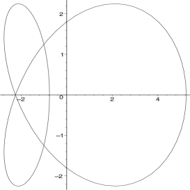
Figure 1. $n=2,\,r=3/2$

Case $r=2$: Figure corresponds the critical case that $|u|=2$ passes through the mixed singular point $(-2,0)$.

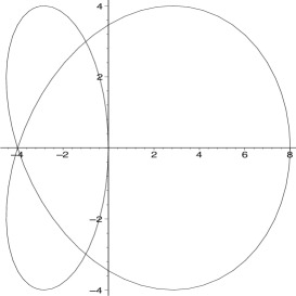
Figure 2. $n=2,\,r=2$

Case $r=3$. The disk $|u|\leq 3$ contains mixed singular point $(-2,0)$ and $\rm{m_{s,tot}}\/(f)=2$.

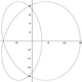
Figure 3. $n=2,\,r=3$

References

- [1] P. Griffiths and J. Harris. Principles of algebraic geometry. Wiley Classics Library. John Wiley & Sons Inc., New York, 1994. Reprint of the 1978 original.
- [2] J. Milnor. Lectures on the -cobordism theorem. Notes by L. Siebenmann and J. Sondow. Princeton University Press, Princeton, N.J., 1965.
- [3] M. Oka. Topology of polar weighted homogeneous hypersurfaces. Kodai Math. J., 31(2):163–182, 2008.
- [4] M. Oka. On mixed projective curves. ArXiv 0910.2523, XX(X), 2009.
- [5] M. Oka. Non-degenerate mixed functions. Kodai Math. J., 33(1):1–62, 2010.