Improved variable selection with Forward-Lasso adaptive shrinkage

Abstract

Recently, considerable interest has focused on variable selection methods in regression situations where the number of predictors, $p$, is large relative to the number of observations, $n$. Two commonly applied variable selection approaches are the Lasso, which computes highly shrunk regression coefficients, and Forward Selection, which uses no shrinkage. We propose a new approach, “Forward-Lasso Adaptive SHrinkage” (FLASH), which includes the Lasso and Forward Selection as special cases, and can be used in both the linear regression and the Generalized Linear Model domains. As with the Lasso and Forward Selection, FLASH iteratively adds one variable to the model in a hierarchical fashion but, unlike these methods, at each step adjusts the level of shrinkage so as to optimize the selection of the next variable. We first present FLASH in the linear regression setting and show that it can be fitted using a variant of the computationally efficient LARS algorithm. Then, we extend FLASH to the GLM domain and demonstrate, through numerous simulations and real world data sets, as well as some theoretical analysis, that FLASH generally outperforms many competing approaches.

TITL1Supported in part by NSF Grants DMS-07-05312 and DMS-09-06784.

and

1 Introduction

Consider the traditional linear regression model

$$Y_{i}=\beta_{0}+\sum_{j=1}^{p}X_{ij}\beta_{j}+\varepsilon_{i},\qquad i=1,\ldots,n,$$ (1)

with $p$ predictors and $n$ observations. Recently attention has focused on the scenario where $p$ is large relative to $n$. In this situation there are many methods that outperform ordinary least squares (OLS) [Frank and Friedman (1993)]. One common approach is to assume that the true number of regression coefficients, that is, the number of nonzero $\beta_{j}$’s, is small, in which case estimation results can be improved by performing variable selection. Many classical variable selection methods, such as Forward Selection, have been proposed. More recently, interest has focused on an alternative class of penalization methods, the most well known of which is the Lasso [Tibshirani (1996)]. In addition to minimizing the usual sum of squares, the Lasso imposes an $L_{1}$ penalty on the coefficients, which has the effect of automatically performing variable selection by setting certain coefficients to zero and shrinking the remainder. While the shrinkage approach can work well, it has been shown that in sparse settings the Lasso often over-shrinks the coefficients. Numerous alternatives and extensions have been suggested. A few examples include SCAD [Fan and Li (2001)], the Elastic Net [Zou and Hastie (2005)], the Adaptive Lasso [Zou (2006)], the Dantzig selector [Candes and Tao (2007)], the Relaxed Lasso [Meinshausen (2007)], VISA [Radchenko and James (2008)] and the Double Dantzig [James and Radchenko (2009)].

The Lasso has been made particularly appealing by the advent of the LARS algorithm [Efron et al. (2004)] which provides a highly efficient means to simultaneously produce the set of Lasso fits for all values of the tuning parameter. The LARS algorithm starts with an empty set of variables and then adds the predictor, say, $\mathbf{X}_{j}$, most highly correlated with the response. Next, the corresponding estimated coefficient, $\hat{\beta}_{j}$, is adjusted in the direction of the least squares solution. The algorithm “breaks” when the absolute correlation between $\mathbf{X}_{j}$ and the residual vector, $\mathbf{Y}-X\hat{\bolds{\beta}}$, is reached by the corresponding correlation for another predictor. The new predictor, say, $\mathbf{X}_{k}$, is then added to the model, and the coefficients $\hat{\beta}_{j}$ and $\hat{\beta}_{k}$ are increased toward their joint least squares solution until some other variable’s correlation matches those of $\mathbf{X}_{j}$ and $\mathbf{X}_{k}$, at which point the new variable is also added to the model. This process continues until all the correlations have reached zero, which corresponds to the ordinary least squares solution.

By comparison, a common version of Forward Selection also starts with an empty model and then iteratively adds to the model the variable most highly correlated with the current residual vector. Next, the residuals are recomputed using the ordinary least squares solution, based on the currently selected variables. This algorithm repeats until all the variables have been added to the model. In comparing Forward Selection with LARS, one observes that the main difference is that the former method drives the regression estimates for the currently selected variables all the way to the least squares solution, while LARS only moves them part way in this direction. Hence, the Lasso estimates the residual vector using shrunk regression coefficients, while Forward Selection uses unshrunk estimates. Which approach is superior? In Section 2 we show that, even for toy examples with no noise in the response, neither universally dominates the other. In some situations the Lasso’s high level of shrinkage produces the best results, while in other cases unshrunk estimates work better.

In this paper we suggest viewing the Lasso and Forward Selection as two extremes on a continuum of possible model selection rules. Instead of selecting candidate models using either highly shrunk or else completely unshrunk coefficients, we propose a methodology that can adaptively adjust the level of shrinkage at each step in the algorithm. We call our approach “Forward-Lasso Adaptive SHrinkage” (FLASH). As with LARS, our algorithm selects the variable most highly correlated with the residuals and drives the selected coefficients toward the least squares solution. However, instead of stopping at the highly shrunk Lasso point or the zero shrinkage Forward Selection point, FLASH uses the data to adaptively choose, at each step, the optimal level of shrinkage before selecting the next variable. FLASH includes Forward Selection and the Lasso as special cases, yet has the same order of computational cost as the Lasso. After introducing FLASH in the linear regression setting, we then extend it to the Generalized Linear Models (GLM) domain. Thus, FLASH can also be used to perform variable selection in high dimensional classification problems using, for example, a logistic regression framework. This significantly expands the range of problems that FLASH can be applied to. We show through extensive simulation studies, as well as theoretical arguments, that FLASH significantly outperforms Forward Selection, the Lasso and many alternative methods, in both the regression and the GLM domains.

Our paper is structured as follows. In Section 2 we demonstrate that neither Forward Selection nor the Lasso universally dominate each other. We present the FLASH methodology in the linear regression setting and outline an algorithm for efficiently constructing its path. Some theoretical properties of FLASH are also discussed. Then in Section 3 we present a detailed simulation study to examine the practical performance of FLASH in comparison to Forward Selection, the Lasso and other competing methods. FLASH is extended to the GLM setting in Section 4 and further simulation results are provided. In Section 5 FLASH is demonstrated on several real world data sets, predicting baseball salaries, real estate prices and whether an internet image is an advertisement. These data sets all have many predictors, up to $p=1430$, and involve both linear regression and GLM scenarios. We end with a discussion in Section 6.

2 Methodology

Using suitable location and scale transformations, we can standardize the data so that the response, $\mathbf{Y}$, and each predictor, $\mathbf{X}_{j}$, are mean zero with $\|\mathbf{X}_{j}\|=1$. Throughout the paper we assume that this standardization holds. However, all numerical results are presented on the original scale of the data.

2.1 Lasso versus Forward Selection

As discussed in the introduction, both the LARS implementation of the Lasso and the Forward Selection algorithm choose the variable with the highest absolute correlation and then drive the selected regression coefficients toward the least squares solution. The key difference is that Forward Selection produces unshrunk estimates by utilizing the least squares solution while the Lasso uses shrunk estimates by only driving the coefficients part way. Which approach works better? It is not hard to show that even in simple settings neither approach dominates the other.

Figure 1: Plots showing regions where the Lasso and Forward Selection will identify the correct model for different correlation structures. Points above the dashed lines correspond to the Lasso regions. Points between the dash dot lines correspond to Forward Selection. The solid lines provide the regions of feasible correlation combinations.

Consider, for example, a scenario involving a linear model with two signal predictors, one noise variable and no error term. Denote by $\rho_{S_{1},S_{2}}$ the correlation between the signal predictors and let $\rho_{S_{i},N_{j}}$ denote the correlation between the $i$th signal and $j$th noise variable. Provided the coefficient for the first signal variable is large enough, this variable is the one most highly correlated with the response, thus it is the first selected by both the Lasso and Forward Selection. In this setting one can directly calculate the values of $\rho_{S_{1},S_{2}},\rho_{S_{1},N_{1}}$ and $\rho_{S_{2},N_{1}}$ where the Lasso or Forward Selection selects the “correct” set of variables. Figure 1 provides an illustration for three different values of $\rho_{S_{1},N_{1}}$. The regions between the dash dot curves correspond to the values of $\rho_{S_{1},S_{2}}$ and $\rho_{S_{2},N_{1}}$ where Forward Selection will identify the correct model. Alternatively, the regions above the dashed curve represent the same situations for the Lasso. The solid lines encompass the regions of feasible correlation combinations. Even in this simplified example it is clear that there are many cases where Forward Selection succeeds and the Lasso fails, and vice versa.

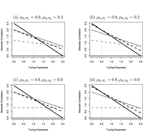
Figure 2: Absolute correlations of the two signal variables (black and gray solid) and two noise variables (black and gray dashed) for different values of $\rho_{S_{1}N_{1}}$ and $\rho_{S_{1}N_{2}}$ in the example considered in Section 2.1. The first dotted vertical indicates the Lasso break point, and the second dotted vertical corresponds to Forward Selection. The line (other than black solid) with the highest value at the break point indicates the variable selected by the corresponding method. The Lasso succeeds only in (a) and (c), and Forward only in (a) and (b).

Figure 2 graphically illustrates how the Lasso, Forward Selection or both methods could fail, using the same simple setup with one additional noise variable. For each plot the four lines represent the absolute correlation between the corresponding variable and the residual vector; solid lines for signal variables and dashed lines for noise variables. The left-hand side of the plot corresponds to the null model with all coefficients set to zero, and the lines show how the correlations change as coefficients are adjusted toward the least squares solution. Each plot represents different values of $\rho_{S_{1},N_{1}}$ and $\rho_{S_{1},N_{2}}$. The values for the other relevant parameters are fixed for all four plots at $\beta_{1}=2,\beta_{2}=1,\rho_{S_{1},S_{2}}=0.5,\rho_{S_{2},N_{1}}=\rho_{S_{2},N_{2}}=0.8$.

In all four plots the black solid line, representing the first signal variable, has the maximal correlation for the null model, so both the Lasso and Forward Selection choose this variable first and drive its coefficient toward the least squares solution. However, the Lasso stops when the black line intersects with one of the other variables and adds that variable next, the first vertical dotted line in each plot, while Forward Selection drives the black line to zero, that is, the least squares solution, and then selects the variable with the maximal correlation, the second dotted line. For a method to choose the correct model it must select the second signal variable, represented by the gray solid line. In Figure 2(a) the gray solid line is the highest at both the Lasso and Forward Selection stopping points, so both methods choose the correct model. However, in Figure 2(b) the Lasso selects the black dashed noise variable, while Forward Selection still chooses the correct model. Alternatively, in Figure 2(c) the Lasso correctly selects the gray signal variable, while Forward Selection chooses the gray dashed noise variable. Finally, in Figure 2(d) both the Lasso and Forward Selection incorrectly select noise variables.

2.2 An adaptive shrinkage methodology

A key observation from Figure 2 is that in all four plots the correct solid grey signal variable has the maximal correlation for at least some levels of shrinkage, even in situations where the Lasso and Forward Selection fail to identify the correct model. This example illustrates that choosing the variable most highly correlated with the residuals can work well provided the correct level of shrinkage is used. This observation motivates our “Forward-Lasso Adaptive SHrinkage” (FLASH) methodology.

Like the Lasso and Forward Selection, FLASH begins with the null model containing no variables and then implements the following procedure:

1. At each step add to the model the variable most highly correlated with the current residual vector.

2. Move the coefficients for the currently selected variables a given distance in the direction toward the corresponding ordinary least squares solution.

3. Repeat steps 1 and 2 until all variables have been added to the model.

The FLASH algorithm is similar to that for LARS and Forward Selection. The main difference revolves around the distance that the coefficients are driven toward the least squares solution. For the $l$th step in the FLASH algorithm this distance is determined by a tuning parameter, $\delta_{l}$. Setting $\delta_{l}=0$ corresponds to the Lasso stopping rule, that is, driving the coefficients until the maximum of their absolute correlations intersect with that of another variable. Alternatively, $\delta_{l}=1$ corresponds to the Forward Selection approach where the coefficients are set equal to the corresponding least squares solution. However, setting $\delta_{l}=\frac{1}{2}$, for example, causes the coefficients to be driven half way between the Lasso and the Forward Selection stopping points. As a result, FLASH can adjust the level of shrinkage not just on the final model coefficients, as used previously in, for example, the Relaxed Lasso, but also at each step during the selection of potential candidate models.

Figure 3: Example coefficient paths for a two variable example using Forward Selection (crosses), the Lasso (triangles) and FLASH (circles).

Figure 3 illustrates potential coefficient paths, for the first two variables selected, for each of the three different approaches. The horizontal solid line in each plot shows the path for the first variable selected, $\beta_{1}$. The first plot illustrates Forward Selection where $\beta_{1}$ is driven all the way to the least squares solution, represented by the first cross. Alternatively, the Lasso (second plot) only drives $\beta_{1}$ a quarter of the way to the least squares solution. Finally, the third plot shows one possible FLASH solution. Here we have marked $\delta_{1}=0$ for the Lasso solution and $\delta_{1}=1$ for the Forward Selection estimate. In this case we set $\delta_{1}=\frac{1}{2}$ and, hence, the corresponding FLASH estimate for $\beta_{1}$ is half way between the Lasso and Forward Selection coefficients. The sloped solid line on each plot illustrates the continuation of the paths to estimate both $\beta_{1}$ and $\beta_{2}$. Again, Forward Selection drives $\beta_{1}$ and $\beta_{2}$ to their joint least squares solution, while the Lasso estimate only moves part way in this direction. The final plot shows the FLASH estimate, again setting $\delta_{2}=\frac{1}{2}$.

In the following section we describe two different approaches for letting the data select the optimal level of shrinkage at each step. In some situations, for example, where a subset of the true variables has a high signal, we may wish to adopt the Forward Selection approach with no shrinkage. In other situations, for example, where there is a lot of noise, the highly shrunk Lasso estimates may be preferred. But, as we show in the simulation results, often a level of shrinkage between these two extremes gives superior results. Another strength of FLASH is that its coefficient path can be efficiently computed using a variant of the LARS algorithm, which we outline next.

We use index $l$ to denote each step of the algorithm, but for simplicity of the notation we omit this index wherever the meaning is clear without it. Throughout the algorithm index set $\mathcal{A}$ represents the correlations that are being driven toward zero, vector $\mathbf{c}_{\mathcal{A}}$ contains the values of these correlations, and $X_{\mathcal{A}}$ denotes the matrix consisting of the columns of $X$ associated with the set $\mathcal{A}$. We refer to this set and the corresponding correlations as “active.” Note that the active absolute correlations are driven toward zero at rates that are proportional to their magnitudes:

1. Initialize ${\bolds{\beta}}^{1}=\bolds{0}$, $\mathcal{A}=\varnothing$ and $l=1$.

2. Update the active set $\mathcal{A}$ by including the index of the (new) maximal absolute correlation. Compute the $|\mathcal{A}|$-dimensional direction vector $\mathbf{h}_{\mathcal{A}}=(X_{\mathcal{A}}^{T}X_{\mathcal{A}})^{-1}\mathbf{c}_{\mathcal{A}}$. Let $\mathbf{h}$ be the $p$-dimensional vector with the components corresponding to $\mathcal{A}$ given by $\mathbf{h}_{\mathcal{A}}$, and the remainder set to zero.

3. Compute $\gamma_{L}$, the Lasso distance to travel in direction $\mathbf{h}$ until a new absolute correlation is maximal. We provide the formulas in the Appendix, where we also show that $\gamma_{F}$, the Forward Selection distance to travel in direction $\mathbf{h}$ until the active correlations reach zero, equals one. Define $\gamma=\gamma_{L}+\delta_{l}(1-\gamma_{L})$ and let ${\bolds{\beta}}^{l+1}={\bolds{\beta}}^{l}+\gamma\mathbf{h}$. Set $l\leftarrow l+1$.

4. Repeat steps 2 and 3 until all correlations are at zero.

Our attention has recently been drawn to the Forward Iterative Regression and Shrinkage Technique (FIRST) in Hwang, Zhang and Ghosal (2009), which can perform effectively in sparse high-dimensional settings. FIRST also utilizes aspects of the Forward Selection and Lasso approaches, but in a rather different fashion than FLASH. For example, in the orthogonal design matrix situation FIRST, when run to convergence, returns the Lasso fit, while FLASH still produces a continuum of solutions between those of the Lasso and Forward Selection.

2.3 Modifications to the algorithm

In practice, we propose implementing FLASH with the following two modifications. First, note that when all $\delta_{l}$ are set to zero, the algorithm above reduces to the basic LARS algorithm, which does not necessarily recover the Lasso path. To ensure that FLASH is a generalization of the Lasso, we implement FLASH using the same modification as the LARS algorithm uses to compute the Lasso path, that is, if at any point on the path a coefficient hits zero, then the corresponding variable is removed from the active set. A detailed description of this modification is given in the Appendix.

Second, to account for the potential over-shrinkage of the coefficients in a sparsely estimated model, we implement a “relaxed” version of FLASH, which extends FLASH analogously to the way that the Relaxed Lasso extends the Lasso. We unshrink each solution located at a breakpoint of the FLASH path, connecting it via a path with the ordinary least squares solution on the corresponding set of variables. We do this as soon as the FLASH breakpoint is computed, in other words, right after the third step of the algorithm. As with the Relaxed Lasso, the calculation of the corresponding relaxation direction comes at no computational cost, as it coincides with the current direction of the FLASH path. More specifically, the original FLASH solution after step 3 is given by ${\bolds{\beta}}^{l}+\gamma\mathbf{h}$, and the corresponding OLS solution is given by ${\bolds{\beta}}^{l}+\mathbf{h}$. The corresponding relaxation path is given by linear interpolation between these two points.

For the remainder of this paper, when we refer to FLASH, we mean the modified version. In our numerical examples the final solution is selected via cross-validation as a point on one of the relaxation paths, where each of these continuous paths is replaced by its values on a fixed grid.

2.4 Selection of tuning parameters

An important component of FLASH is the selection of the $\delta_{l}$ parameters. Clearly, treating each $\delta_{l}$ as an independent tuning parameter is not feasible. Many model selection approaches could be utilized. In this paper we investigate two possible approaches. The first, “global FLASH,” involves selecting a single value, $\delta$, for all the step sizes, that is, assuming a common level of shrinkage throughout the steps of the FLASH algorithm. Hence, $\delta=0$ corresponds to the Lasso and $\delta=1$ to Forward Selection. Using this approach, we first choose a grid of $\delta$’s between $0$ and $1$ and then select the value giving the lowest residual sum of squares on a validation data set or, alternatively, the lowest cross-validated error. Global FLASH has the advantage of only needing to select one $\delta$, which improves its computational efficiency.

The second approach, “block FLASH,” allows for different values among the $\delta_{l}$’s. However, to make the problem computationally feasible, we constrain each $\delta_{l}$ to be either zero or one. The version of block FLASH we focus on exclusively for the remainder of the paper involves selecting a single “break point” with $\delta_{l^{*}}=1$ and setting all remaining $\delta_{l}$’s to zero. This has the effect of dividing FLASH into two stages. In the first stage a series of Lasso steps (i.e., $\delta_{l}=0$) are performed to select the initial variables. At the end of the first stage a Forward step (i.e., $\delta_{l^{*}}=1$) is performed which has the effect of removing the coefficient shrinkage on the currently selected variables. In the second stage further variables are selected by performing a series of Lasso steps. As with global FLASH, block FLASH has the advantage of only needing to select one tuning parameter, the break point. In Section 3 we provide simulation results for both versions of FLASH. In practice, the two methods appear to perform similarly. However, as illustrated below, we are able to establish some interesting theoretical properties for block FLASH.

Note that for each fixed $\delta$ or, correspondingly, each fixed $l^{*}$, global and block FLASH both have the same computational cost as the LARS algorithm. Because LARS is extremely efficient, so are the FLASH algorithms, in particular, they require the same order of calculations as LARS if the grid size for $\delta$ and the number of locations for $l^{*}$ are finite. We propose using a five value grid for $\delta$, which worked very well in our simulation study. The upper bound on the number of potential locations for $l^{*}$ can be chosen based on the computational complexity of the problem. Remember that $l^{*}$ represents the number of easily identifiable predictors, so one might reasonably expect a relatively low value.

2.5 Theoretical arguments

In this section we present some variable selection properties of FLASH, in particular, conditions under which it can be shown to outperform the Lasso. Throughout this section “probability tending to one” refers to the scenario of $p$ going to infinity. For the standard case of bounded $p,$ we could think of $n$ going to infinity instead, although some minor modifications would need to be made to the statements of the results. Let $K$ index the nonzero coefficients of ${\bolds{\beta}}$. We will say that an estimator $\widehat{{\bolds{\beta}}}$ recovers the correct signed support of ${\bolds{\beta}}$ if $\operatorname{sign}(\widehat{{\bolds{\beta}}})=\operatorname{sign}({\bolds{\beta}})$, where the equality is understood componentwise.

We will take a common approach of imposing bounds on the maximum absolute correlation between two predictors. Define $S$ as the number of signal variables, $\mu=\max_{j>k}|\mathbf{X}_{j}^{T}\mathbf{X}_{k}|$ and let $\xi$ be an arbitrarily small positive constant. The results of Zhao and Yu (2006) and Wainwright (2009) imply that if

$$\min_{j\in K}|\beta_{j}|>c_{1}\sqrt{S\log p}$$ (2)

and $\mu<\mu_{\mathrm{L}}(1-\xi)$ with $\mu_{\mathrm{L}}=1/[2S-1]$, then the Lasso solution corresponding to an appropriate choice of the tuning parameter will recover the correct signed support of ${\bolds{\beta}}$ with probability tending to one. Here the constant $c_{1}$ does not change with $n$ and $p$, and its value is provided in the supplemental article [Radchenko and James (2010)]. On the other hand, the number of true nonzero coefficients, $S$, is allowed to grow together with $n$ and $p$. Note that condition (2) is stated for the rescaled coefficients that correspond to the standardized predictor vectors. On the original scale the right-hand side in (2) would be of order $\sqrt{(S\log p)/n}$. Suppose, for example, that $S$ is bounded and $p$ grows polynomially in $n$. In this case the lower bound on the magnitudes of the nonzero coefficients, expressed on the original scale, goes to zero at the rate $\sqrt{(\log n)/n}$.

The correlation bound above is tight in the sense that for each $\mu\geq\mu_{L}$ there are values of $X^{T}X$ and sign$({\bolds{\beta}})$ such that the Lasso fails to recover the correct signed support. In the following claim we identify a class of such counterexamples.

Claim 1

Let $\rho$ be a constant satisfying $\rho\geq\mu_{L}$ and let $j$ be an arbitrary index in $K^{c}$. Suppose that all the pairwise correlations among the predictors indexed by $K\cup\{j\}$ equal $-\rho$, and all the signs of the nonzero coefficients of ${\bolds{\beta}}$ are negative. Then, with probability at least $1/2$, no Lasso solution recovers the correct signed support of ${\bolds{\beta}}$.

The proof of the claim is provided in the supplemental article [Radchenko and James (2010)]. Note that for $\rho<1/S$ the correlation matrix can be easily made positive definite by setting all the nonspecified pairwise correlations to zero.

Our Theorem 1 establishes that, under an additional assumption on the magnitudes of the nonzero coefficients, block FLASH can work in the situations where the Lasso fails. The intuition behind this additional assumption is that for many regression problems there will be some signal variables that are relatively easy to identify, while the remainder pose more difficulties. The block FLASH procedure utilizes the first group of signal variables in a more efficient fashion and hence is better able to identify the remaining predictors. To mathematically quantify this intuition, suppose that there exist indexes $a$ and $b$, such that the corresponding true coefficients are nonzero and have a significant separation in the magnitudes, that is, a large value of $|\beta_{a}/\beta_{b}|$. We will refer to the coefficients $\{\beta_{j}\dvtx|\beta_{j}|\geq|\beta_{a}|\}$ as large, and the coefficients $\{\beta_{j}\dvtx 0<|\beta_{j}|\leq|\beta_{b}|\}$ as small. Theorem 1 below states that if the ratio $|\beta_{a}/\beta_{b}|$ is sufficiently large, then the block FLASH procedure will correctly identify the signal variables under a weaker assumption on the maximal pairwise correlation. More specifically, at the first stage the procedure will identify all the large nonzero coefficients and not pick up any noise, and at the second stage it will pick up the remaining nonzero coefficients without bringing in the noise. As we discuss at the end of the section, the new correlation bound, $\mu_{\mathrm{FL}}$, is strictly larger than the Lasso bound, $\mu_{\mathrm{L}}$.

Theorem 1

Suppose that condition (2) holds, inequality $|\beta_{a}/\beta_{b}|>c_{3}\sqrt{S}$ is satisfied for an arbitrary pair of true nonzero coefficients, and $\mu<\mu_{\mathrm{FL}}(1-\xi)$ for some arbitrary constant $\xi$. Then, with an appropriate choice of the tuning parameters, the block FLASH estimator recovers the correct signed support of ${\bolds{\beta}}$ with probability tending to one.

Here the constant $c_{3}$ does not change with $n$ and $p$, and its value is provided in the supplemental article [Radchenko and James (2010)] together with the proof of the theorem. Like the corresponding Lasso result in Wainwright (2009), our theorem can handle subgaussian errors, that is, the tails of the error distribution are required to decay at least as fast as those of a gaussian distribution. Relative to the Lasso result, the only new assumption is on the separation between the large and the small coefficients. Consequently, we are able to relax the requirement on the pairwise correlations. According to Claim 1, the new assumption does not allow us to relax the pairwise correlation requirement for the Lasso, as the nonzero coefficients of ${\bolds{\beta}}$ affect the claim only through their signs. Applying Theorem 1 in the setup of the claim yields that the correct signed support of ${\bolds{\beta}}$ can be recovered for all $\rho<\mu_{\mathrm{FL}}$. In other words, under an additional assumption on the magnitudes of the nonzero coefficients, block FLASH succeeds for $\rho\in[\mu_{\mathrm{L}},\mu_{\mathrm{FL}})$, where the Lasso fails.

The correlation bound in Theorem 1 can be taken as

$$\mu_{\mathrm{FL}}=\min\biggl{\{}\frac{1}{2(1-q_{2})S-1},\frac{1}{(2-q_{1})S}\biggr{\}}.$$ (3)

Here $q_{1}$ and $q_{2}$ are the fractions of large and small coefficients, respectively, among all the nonzero coefficients. More specifically, $q_{1}=|\{\beta_{j}\dvtx|\beta_{j}|\geq|\beta_{a}|\}|/S$ and $q_{2}=|\{\beta_{j}\dvtx 0<|\beta_{j}|\leq|\beta_{b}|\}|/S$. Observe that $\mu_{\mathrm{FL}}>\mu_{\mathrm{L}}$ when $q_{1}S>1$. In fact, the proof of Theorem 1 reveals that the best possible value of $\mu_{\mathrm{FL}}$ is strictly above $\mu_{\mathrm{L}}$ for all positive $q_{1}$.

3 Simulation results

In this section we present a detailed simulation study comparing FLASH to five natural competing approaches. We implemented both the global (FLASH_G) and the block (FLASH_B) versions of our method discussed in Section 2.4. The tuning parameter $\delta$ in FLASH_G was selected from a grid of five possible values, $\{0,0.25,0.5,0.75,1\}$. We also tried a $\{0,1\}$ grid corresponding to the Lasso and Forward Selection, and a $\{0,0.5,1\}$ grid, but the results were inferior, so we do not report them here.

We compared FLASH to VISA, the Relaxed Lasso (Relaxo), the Adaptive Lasso (Adaptive), Forward Selection (Forward) and the Lasso. The Adaptive Lasso involves a preliminary step where the weights are typically chosen by performing a least squares fit to the data. This is not feasible for $p>n$, so we selected the weights using either the simple linear regression fits, as suggested in Huang, Ma and Zhang (2008), or a ridge regression fit, as suggested in Zou (2006). The ridged fits dominated so we only report results for the latter method here.

Our simulated data consisted of five parameters which we varied: the number of variables ($p=100$ or $p=200$), the number of training observations ($n=50,n=70$ or $n=100$), the correlations among the columns of the design matrix ($\rho=0$ or $\rho=0.5$), the number of nonzero regression coefficients ($S=10$ or $S=30$) and the standard deviation among the coefficients ($\sigma_{\beta}=0.5,\sigma_{\beta}=0.7$ or $\sigma_{\beta}=1$). We tested most combinations of the parameters and report a representative sample of the results. The rows of the design matrix were generated from a mean zero normal distribution with a correlation matrix whose off-diagonal elements were equal to $\rho$. The error terms were sampled from the standard normal distribution, while the regression coefficients were generated from a mean zero normal with variance $\sigma_{\beta}^{2}$. For each simulated data set we randomly generated a validation data set with half as many observations as the training data and selected the various tuning parameters for each method as those that gave the lowest mean squared error between the response and predictions on the validation data. In particular, both the relaxation parameter and the number of steps in the algorithm for the FLASH methods and the Relaxed Lasso were selected using a validation set. For each method and simulation we computed three statistics, averaged over $200$ data sets: False Positive, the number of variables with zero coefficients incorrectly included in the final model; False Negative, the number of variables with nonzero coefficients left out of the model; and L2 square, the squared $L_{2}$ distance between the estimated coefficients and the truth. Table 1 provides the results.

Table 1: Simulation results for each method. L2 square denotes the squared $L_{2}$ distance between the estimated coefficients and the truth, averaged over the 200 simulated data sets. For each simulation scenario we placed in bold the best L2 square value together with the L2 square value for any other method that was not statistically worse at the $5\%$ level of significance

Simulation	Statistic	FLASHG	FLASHB	VISA	Relaxo	Adaptive	Forward	Lasso
$n=100$, $p=100$	False-Pos	$1.92$	$3.32$	$3.23$	$3.7$	$9.9$	1.11	$18.68$
$S=10$, $\rho=0$	False-Neg	$2.12$	$1.89$	$2.26$	$2.26$	$1.84$	2.33	$1.27$
$\sigma_{\beta}=1$	L2-sq	0.249	0.249	$0.292$	$0.308$	$0.342$	0.244	$0.436$
$n=100$, $p=200$	False-Pos	$1.99$	$3.91$	$3.53$	$3.87$	$12.61$	1.07	$21.18$
$S=10$, $\rho=0$	False-Neg	$2.32$	$2.09$	$2.44$	$2.45$	$2.44$	2.48	$1.64$
$\sigma_{\beta}=1$	L2-sq	0.267	$0.286$	$0.353$	$0.366$	$0.524$	0.266	$0.606$
$n=50$, $p=100$	False-Pos	$2.65$	$6.17$	$4.88$	$5.1$	$10.39$	1.71	$15.41$
$S=10$, $\rho=0$	False-Neg	$3.3$	$2.9$	$3.38$	$3.4$	$3.08$	3.79	$2.42$
$\sigma_{\beta}=1$	L2-sq	0.775	$0.848$	$0.996$	$1.021$	$1.228$	00.929	$1.285$
$n=50$, $p=200$	False-Pos	$3.73$	$7.24$	$6.46$	$6.84$	$12.89$	1.71	$18.54$
$S=10$, $\rho=0$	False-Neg	$3.83$	$3.4$	$4.06$	$4.04$	$3.81$	4.57	$3.04$
$\sigma_{\beta}=1$	L2-sq	1.057	1.089	$1.477$	$1.496$	$1.999$	01.365	$1.934$
$n=100$, $p=100$	False-Pos	$3.13$	$4.79$	$6.33$	$6.53$	$10.41$	1.32	$19.66$
$S=10$, $\rho=0.5$	False-Neg	$2.59$	$2.33$	$2.48$	$2.45$	$2.21$	3.02	$1.62$
$\sigma_{\beta}=1$	L2-sq	0.527	0.546	$0.629$	$0.656$	$0.661$	00.581	$0.797$
$n=100$, $p=200$	False-Pos	$3.35$	$6.35$	$7.06$	$7.33$	$11.82$	1.27	$21.72$
$S=10$, $\rho=0.5$	False-Neg	$3.12$	$2.88$	$3.06$	$3.11$	$3.01$	3.57	$2.23$
$\sigma_{\beta}=1$	L2-sq	0.608	$0.673$	$0.752$	$0.785$	$0.872$	00.655	$1.029$
$n=50$, $p=100$	False-Pos	$5.12$	$8.31$	$7.23$	$7.44$	$11.27$	2.42	$16.2$
$S=10$, $\rho=0.5$	False-Neg	$3.95$	$3.38$	$3.79$	$3.88$	$3.53$	4.82	$2.99$
$\sigma_{\beta}=1$	L2-sq	1.732	1.743	$1.84$	$1.901$	$2.088$	2.38	$2.199$
$n=50$, $p=200$	False-Pos	$5.82$	$9.62$	$8.8$	$8.77$	$12.91$	2.37	$18.28$
$S=10$, $\rho=0.5$	False-Neg	$5.14$	$4.45$	$5.04$	$5.12$	$4.9$	6.25	$4.34$
$\sigma_{\beta}=1$	L2-sq	2.399	2.35	$2.648$	$2.7$	$2.851$	03.094	$2.934$
$n=50$, $p=100$	False-Pos	$10.6$	$13.73$	$11.34$	$12.09$	$15.62$	4.39	$17.16$
$S=30$, $\rho=0$	False-Neg	$14.23$	$12.1$	$14.12$	$13.89$	$12.91$	21.7	$11.95$
$\sigma_{\beta}=1$	L2-sq	$10.559$	9.051	$10.749$	$10.743$	$11.132$	19.792	$11.316$
$n=100$, $p=100$	False-Pos	$3.54$	$4.72$	$6.09$	$6.19$	$10.52$	1.84	$17.86$
$S=10$, $\rho=0.5$	False-Neg	$3.73$	$3.54$	$3.51$	$3.56$	$3.34$	4.24	$2.46$
$\sigma_{\beta}=0.7$	L2-sq	0.625	0.624	$0.692$	$0.705$	$0.724$	00.707	$0.787$
$n=100$, $p=200$	False-Pos	$4.06$	$6.21$	$7.11$	$7.48$	$11.69$	1.68	$21.46$
$S=10$, $\rho=0.5$	False-Neg	$4.05$	$3.81$	$3.87$	$3.93$	$3.7$	4.68	$3$
$\sigma_{\beta}=0.7$	L2-sq	0.686	$0.731$	$0.788$	$0.794$	$0.799$	0.77	$0.922$
$n=100$, $p=100$	False-Pos	$3.81$	$4.88$	$6.11$	$5.93$	$9.65$	1.99	$15.78$
$S=10$, $\rho=0.5$	False-Neg	$4.74$	$4.49$	$4.46$	$4.51$	$4.16$	5.48	$3.42$
$\sigma_{\beta}=0.5$	L2-sq	0.559	0.545	$0.576$	$0.584$	$0.596$	00.683	$0.633$
$n=100$, $p=200$	False-Pos	$3.69$	$5.25$	$5.76$	$6.13$	$10.11$	1.54	$17.73$
$S=10$, $\rho=0.5$	False-Neg	$5.38$	$5.08$	$5.29$	$5.32$	$4.88$	6.03	$4.24$
$\sigma_{\beta}=0.5$	L2-sq	0.664	0.662	0.696	$0.709$	$0.715$	00.761	$0.769$

The first four simulations corresponded to $\rho=0$, while the next four were generated using $\rho=0.5$. The ninth simulation was a denser case with $S=30$. Finally, the last four simulations represent harder problems with $\sigma_{\beta}=0.7$ or $0.5$, reducing the signal to noise ratio from $10$ to $4.9$ and $2.5$, respectively. For the L2 square statistic we performed tests of statistical significance, comparing each method to the best FLASH approach. For each simulation we placed in bold the L2 square value for the best method and any other method that was not statistically worse at the $5\%$ level of significance. For example, in the first simulation with $100$ variables and $100$ observations both versions of FLASH and Forward were statistically indistinguishable from each other. However, in the third simulation with $100$ variables and $50$ observations FLASH_G was statistically superior to all other methods. Most of the standard errors for the L2 square statistic were relatively low, approximately $4\%$ of the statistic’s value. However, as has been observed previously, we found that the Forward method often gave more variable estimates than the other approaches, with some standard errors as high as $8\%$ of the statistic’s value.

None of the thirteen simulations contained a situation where one of the competing methods was statistically superior to FLASH, while in ten of the simulations FLASH was statistically superior to all other methods. In general, Forward Selection performed well in the easiest scenarios with large $n$, zero correlation, $\rho$, and higher signal, $\sigma_{\beta}=1$. In particular, Forward Selection performed very poorly in the denser $S=30$ scenario, while this was a favorable situation for the Lasso. FLASH was still superior to both methods in this simulation setup. The Adaptive Lasso, VISA and Relaxo all provided improvements over the Lasso, though the latter two methods generated the largest increase in performance. The two versions of FLASH performed at a similar level, though FLASH_G seemed slightly better in the sparser cases, while FLASH_B was superior in the denser $S=30$ situation. FLASH_G also required less computational effort, because its path only needed to be computed once for each of the five potential values of $\delta$.

Overall, Forward Selection had low false positive but high false negative rates. In comparison to VISA and Relaxo, FLASH_G had the lowest false positive rates and similar or lower false negative rates. Alternatively, FLASH_B had very low false negative rates and similar false positive rates. Overall, FLASH selected sparser models than VISA, the Relaxed Lasso and the Adaptive Lasso, and significantly sparser models than the Lasso.

4 Extending to generalized linear models

4.1 Methodology

In the generalized linear model framework for a response variable, $Y$, with distribution

$$p(y;\theta,\phi)=\exp\biggl{(}\frac{y\theta-b(\theta)}{a(\phi)}+c(y,\phi)\biggr{)},$$

one models the relationship between predictor and response as $g(\mu_{i})=\sum_{j=1}^{p}X_{ij}\beta_{j}$, where $\mu_{i}=E(Y;\theta_{i},\phi)=b^{\prime}(\theta_{i})$, and $g$ is referred to as the link function. Common examples of $g$ include the identity link used for normal response data and the logistic link used for binary response data. For notational simplicity we will assume that $g$ is chosen as the canonical link, though all the ideas generalize naturally to other link functions. The coefficient vector ${\bolds{\beta}}$ is generally estimated by maximizing the log likelihood function,

$$l({\bolds{\beta}})=\sum_{i=1}^{n}\bigl{(}Y_{i}\mathbf{X}_{i}^{T}{\bolds{\beta}}-b(\mathbf{X}_{i}^{T}{\bolds{\beta}})\bigr{)}.$$ (4)

However, when $p$ is large relative to $n$, the maximum likelihood approach suffers from problems similar to those of the least squares approach in linear regression. First, maximizing (4) will not produce any coefficients that are exactly zero, so no variable selection is performed. As a result, the final model is less interpretable and probably less accurate. Second, for large $p$ the variance of the estimated coefficients will become large and when $p>n$, function (4) has no unique minimum.

Various solutions have been proposed. Park and Hastie (2007) discuss a natural GLM extension of the Lasso (GLasso) where, for a fixed $\lambda$, they choose ${\bolds{\beta}}$ to minimize

$$l({\bolds{\beta}},\lambda)=-l({\bolds{\beta}})+\lambda\|{\bolds{\beta}}\|_{1}.$$ (5)

The coefficient paths for the GLasso are not generally piecewise linear, but Park and Hastie present an algorithm for approximating the true path. Forward Selection can also be easily extended to the GLM domain by starting with an empty set of variables and, at step $l$, adding to the model the variable that maximizes the $j$th partial derivative of the log likelihood, $l^{\prime}_{j}(\hat{\bolds{\beta}}_{l})$. One then sets $\hat{\bolds{\beta}}_{l+1}$ equal to the maximum likelihood solution corresponding to the currently selected variables and repeats. Note that $l^{\prime}_{j}(\hat{\bolds{\beta}}_{l})=\mathbf{X}_{j}^{T}(\mathbf{Y}-\hat{\mu})$, which is just the correlation between the $j$th predictor and the residuals. When using Gaussian errors with the identity link function, $\hat{\mu}=X{\bolds{\beta}}$, so this algorithm reduces back to standard Forward Selection in the regression setting.

Figure 4: Example coefficient paths for a two variable GLM example using Forward Selection (crosses), the Lasso (triangles) and FLASH (circles).

The GLM versions of the Lasso and Forward Selection also suggest a natural extension of FLASH to this domain. In the GLM FLASH algorithm we again start with an empty set of variables, $\mathcal{A}_{1}$, and $\hat{\bolds{\beta}}_{1}=\bolds{0}$. Then at step $l$ we add to the model the variable that maximizes the $j$th partial derivative of the log likelihood, $l^{\prime}_{j}(\hat{\bolds{\beta}}_{l})$, that is, the variable with maximal correlation. Finally, we drive $\hat{\bolds{\beta}}_{l+1}$ in the direction toward the maximum likelihood solution with the distance determined by $\delta_{l}$. Again, $\delta_{l}=0$ corresponds to shifting $\hat{\bolds{\beta}}_{l}$ as far as the Lasso stopping point, while $\delta_{l}=1$ represents the maximum likelihood solution. However, one key difference between the GLM and standard versions of FLASH is that, because the coefficient paths are no longer piecewise linear, the coefficients do not move in a linear fashion toward the maximum likelihood solution.

Figure 4 provides a pictorial example in the same two variable domain as for Figure 3. The GLasso still significantly shrinks the coefficients relative to the Forward Selection approach. Alternatively, FLASH provides an in between level of shrinkage. However, notice that the coefficient paths now move in a curved fashion toward the maximum likelihood solution. It is possible to compute this nonlinear path on a grid of tuning parameters, and we present the precise algorithm in the Appendix.

The block FLASH approach is particularly appealing in the GLM setting, because it is both conceptually simple and easy to implement. With this method FLASH follows the GLasso path for the first $l^{*}-1$ steps, that is, $\delta_{1}=\delta_{2}=\cdots=\delta_{l^{*}-1}=0$. At this point the maximum likelihood solution for the currently selected variables is computed, that is, $\delta_{l^{*}}=1$. Finally, the GLasso path is followed again with zero penalty on the variables corresponding to $\mathcal{A}_{l^{*}}$, that is, $\delta_{l^{*}+1}=\cdots=0$. We compute the GLM version of block FLASH using two implementations of the R function $\operatorname{glmnet}(\cdot)$ [Friedman, Hastie and Tibshirani (2010)], which uses a coordinate descent algorithm to minimize (5). We first use $\operatorname{glmnet}(\cdot)$ to compute the path prior to $l^{*}$ and then make a second call to the function to compute the path after $l^{*}$, placing zero penalty on the variables selected in the first step.

4.2 Simulation study

In this section we provide a simulation comparison of the block GLM FLASH method with several other standard GLM approaches. In particular, we compared FLASH to “GLasso,” “GRelaxo,” “GForward” and the standard “GLM.” GLasso is implemented using the R function $\operatorname{glmnet}(\cdot)$. GRelaxo takes the same sequence of models suggested by GLasso but unshrinks the final coefficient estimates using a standard GLM fit to the nonzero coefficients. GForward uses the approach outlined previously.

We simulated responses from the Bernoulli distribution using the logistic link function. The data were generated with $p=100$ variables, but we increased the sample size to $n=400$ as the Bernoulli response provided less information compared to the Gaussian response. The correlation among the predictors was set to either $\rho=0$ or $\rho=0.5$, and the number of true signal variables was set to either $S=10$ or $S=15$. Finally, the nonzero regression coefficients were randomly sampled from either a point mass distribution, with probability a half of being $0.5$ or $-0.5$, or the standard normal distribution. The tuning parameters for all methods were selected as those that minimized the “deviance” on a validation data set with $n=200$ observations. In all other respects the simulation setup was the same as the one we used in the linear regression setting.

Table 2: Simulation results for each method using a Bernoulli response. L2 square denotes the squared $L_{2}$ distance between the estimated coefficients and the truth, averaged over the 200 simulated data sets. For each simulation scenario we placed in bold the best L2 square value together with the L2 square value for any other method that was not statistically worse at the $5\%$ level of significance

Simulation	Statistic	FLASHB	GRelaxo	GLasso	GForward	GLM
$n=400$, $p=100$	False-Pos	4.380	$4.47$	$16.61$	$1.18$	$90$
$S=10$, $\rho=0$	False-Neg	0.340	$0.45$	$0.06$	$0.55$	$0$
$\beta=\pm 0.5$	L2-sq	0.461	$0.488$	$0.71$	0.454	$6.065$
$n=400$, $p=100$	False-Pos	9.100	$10.11$	$15.57$	$1.54$	$90$
$S=10$, $\rho=0.5$	False-Neg	1.690	$1.82$	$0.92$	$3.51$	$0$
$\beta=\pm 0.5$	L2-sq	1.081	$1.147$	1.107	$1.415$	$10.559$
$n=400$, $p=100$	False-Pos	2.940	$3.22$	$17.88$	$0.6$	$90$
$S=10$, $\rho=0$	False-Neg	2.940	$3.07$	$1.8$	$3.24$	$0$
$\beta=N(0,1)$	L2-sq	0.72	$0.779$	$1.954$	0.668	$99.794$
$n=400$, $p=100$	False-Pos	5.370	$7.63$	$17.41$	$0.74$	$90$
$S=10$, $\rho=0.5$	False-Neg	3.210	$3.21$	$2.17$	$4.08$	$0$
$\beta=N(0,1)$	L2-sq	1.168	$1.392$	$1.967$	$1.289$	$58.08$
$n=400$, $p=100$	False-Pos	4.420	$5.8$	$15.55$	$0.7$	$85$
$S=15$, $\rho=0.5$	False-Neg	5.570	$5.38$	$3.66$	$6.81$	$0$
$\beta=N(0,1)$	L2-sq	2.302	$2.692$	$4.211$	$2.487$	$11903.88$

The results from five different simulations are provided in Table 2. Standard GLM performs very poorly. Note we have reported the median errors for this method because the algorithm did not converge properly for some simulations. GForward was competitive with FLASH_B when using uncorrelated predictors but deteriorated in the correlated situation. In all scenarios FLASH_B either had the lowest L2-sq statistic or was not statistically different from the best. In the last two simulations it was statistically superior to all the other approaches.

5 Empirical analysis

We implemented the global, block and GLM versions of FLASH on three different real world data sets. The first contained salaries of professional baseball players (obtained from StatLib, Department of Statistics, CMU). For each player a number of statistics were recorded, such as career runs batted in, walks, hits, at bats, etc. We then used these variables to predict salaries. After including all possible interaction terms, the data set contained $n=263$ observations and $p=153$ predictors.

We tested three competitors to FLASH, namely, Lasso, Forward Selection and the Relaxed Lasso. For each of the four methods ten-fold cross-validation was used to compute the root mean squared error (RMSE) in prediction accuracy at various points of the coefficient path. The final results are illustrated in Figure 5(a). The open circles represent the Lasso RMSE’s evaluated at the break points of the LARS algorithm. Alternatively, the solid circles show the errors corresponding to the least squares fits for the models selected by the Lasso. The dashed line that connects the open and the solid circles illustrates the Relaxed Lasso fit as the coefficient shrinkage is reduced from the Lasso estimate (maximum shrinkage) to the least squares fit (no shrinkage). The dotted line corresponds to Forward Selection. Finally, the black solid line represents the global FLASH fit with $\delta=0.25$. We have fixed the value of the $\delta$ parameter to ensure fair comparison with other methods on the basis of the cross-validated RMSE. In our simulations we used a five point grid, where the end points corresponded to the Relaxed Lasso and Forward Selection, respectively. Among the remaining three values, we decided to pick $\delta=0.25$, as it is closer to the Relaxed Lasso, which is in general a more reliable method then Forward Selection.

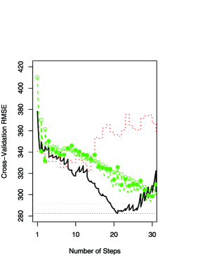
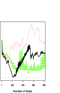
(a)	(b)

Figure 5: (a) The cross-validated root mean squared error plotted versus the number of steps in the corresponding algorithm for four different methods in the example of predicting baseball players’ salary. The methods displayed are Forward Selection (dotted line), Lasso (open circles), OLS fits corresponding to the Lasso models (solid circles), Relaxed Lasso (dashed line, connecting the open and the solid circles) and FLASH with $\delta=0.25$ (solid black line). (b) Same as (a) with more steps.

From step 15 onward, Forward Selection begins to significantly deteriorate, while FLASH continues to improve and eventually achieves the lowest error rate of all four methods at approximately step 20. Figure 5(b) plots the cross-validated error paths out to 80 steps. The Relaxed Lasso achieves its optimal results at approximately step 50, which corresponds to a $34$ variable model. Not only is the optimal error rate worse than that for FLASH, but the corresponding model contains twice as many variables as the model selected by FLASH, which only had $17$ variables. Our simulation results pointed to a similar phenomenon, and we have noticed in other real data sets that FLASH tends to select sparser models, suggesting FLASH may have an advantage in terms of inference in addition to prediction accuracy.

The second data set we examined was the Boston Housing data, commonly used to compare different regression methods. After including interaction terms this data contained $90$ predictors of the average house value in $506$ locations. To test the $p\approx n$ scenario, $90$ observations were randomly sampled for the training data, $45$ observations for a validation data set, and the remainder for the testing data. We implemented the block FLASH approach and compared it to the Lasso, Relaxo and Forward Selection. Least squares fits were used for the final coefficient estimates on all methods except the Lasso. Hence, for example, the Relaxed Lasso solutions simplify to the OLS solutions computed for the sequence of models specified by the Lasso. Each approach was fitted using the training data, with the tuning parameters chosen using the validation data, and then the mean squared error was computed on the test data. This procedure was repeated using $100$ different random samplings of the data, to average out any effect from the choice of test sets. Table 3 shows, for each method, the average mean squared error as well as the average number of coefficients chosen in the final model. Block FLASH achieves the lowest mean squared error. In addition, FLASH, Relaxo and Forward Selection all choose significantly smaller models than the Lasso, making their results more interpretable. On average, block FLASH selected $8.67$ variables before implementing the Forward step. FLASH resulted in lower MSE than Relaxo in 62 random splits of the data, the two methods had the same MSE in 3 splits, and FLASH had a higher MSE in 35 of the splits. The corresponding numbers comparing FLASH to the Lasso and FLASH to Forward Selection were 63/0/37 and 81/0/19.

=250pt FLASH Relaxo Lasso Forward MSE 27.01 28.30 29.56 33.03 Number of coefficients 18.93 17.13 26.99 16.80

Table 3: Mean squared errors, averaged over $100$ test data sets, and average number of variables selected, for the Boston Housing data

The final data set that we examined was the internet advertising data available at the UC-Irvine machine learning repository. The response was categorical, indicating whether or not each image was an advertisement. The predictors recorded the geometry of the image as well as whether certain phrases occurred in and around the image url’s. After preprocessing, the data set contained $n=2359$ observations and $p=1430$ variables. The large value of $p$ presented significant statistical and computational difficulties for standard approaches, with the $\operatorname{glm}(\cdot)$ function in R taking almost fifteen minutes to run and producing NA estimates for most coefficients. However, we were able to implement GLM block FLASH, randomly assigning two-thirds of the observations to the training data set and the remainder to the validation data set. FLASH selected a twenty-seven variable model, with the five most important variables, in terms of the order that they entered the model, being the width of the image, whether the image’s anchor url contained the phrase “com,” whether the url contained the phrase “ads,” and whether the anchor url contained the phrases “click” and “adclick.” We also fixed the tuning parameters at the selected values and used a bootstrap analysis to produce pointwise confidence intervals on the coefficients. GLM block FLASH ran very efficiently, taking approximately twenty seconds to produce the corresponding estimator on each bootstrapped data set. The misclassification error on the validation set was $2.9\%$ for FLASH, while it was $3.2\%$, $4.0\%$ and $5.0\%$, for GRelaxo, GLasso and GForward, respectively. The sizes of the models selected by the last three methods were $38$, $77$ and $16$, respectively.

6 Discussion

The main difference between Forward Selection and the Lasso is in the amount of shrinkage used to iteratively estimate the regression coefficients. For any given data set there is no particular reason that either the zero shrinkage of Forward Selection or the extreme shrinkage of the Lasso must produce the best solution. FLASH allows the data to dictate the optimal level of shrinkage at the model selection stage. This is quite different from approaches such as Relaxo that adjust the level of shrinkage after the model has been selected but not while choosing the sequence of models to consider. As a result, FLASH often produces sparser models with superior predictive accuracy.

Computational efficiency is always important for high-dimensional problems. The standard FLASH algorithm is very similar to LARS and hence involves a relatively small computational expense. In addition, the block FLASH approach can easily be formulated as a penalized regression problem with the usual $L_{1}$ penalty before the Forward step and zero penalty on certain variables after this step. Hence, even more efficient methods, such as the recent work on pathwise coordinate descent algorithms [Friedman et al. (2007)], can be used to compute the path, not only for regression problems, but also for our extension to GLM data. Indeed, the $\operatorname{glmnet}(\cdot)$ function that we used to fit GLM block FLASH utilizes a coordinate descent algorithm.

Appendix A Step 3 of the FLASH algorithm

Let $c_{i*}$ be one of the active correlations with the maximum absolute value. Then, as with LARS, the first time a nonactive absolute correlation reaches the “active” maximum corresponds to the step size of

$$\gamma_{L}=\min^{+}_{j\in\mathcal{A}^{c}}\biggl{\{}\frac{c_{i*}-c_{j}}{(\mathbf{X}_{i*}-\mathbf{X}_{j})^{T}X\mathbf{h}},\frac{c_{i*}+c_{j}}{(\mathbf{X}_{i*}+\mathbf{X}_{j})^{T}X\mathbf{h}}\biggr{\}},$$

where the minimum is taken over the positive components.

Along the direction $\mathbf{h}$, all active correlations reach zero at the same time. Hence, the Forward Selection step size is given by

$$\gamma_{F}=\frac{c_{i*}}{\mathbf{X}_{i*}^{T}X\mathbf{h}}=\frac{c_{i*}}{\mathbf{X}_{i*}^{T}X_{\mathcal{A}}(X^{T}_{\mathcal{A}}X_{\mathcal{A}})^{-1}\mathbf{c}_{\mathcal{A}}}=1.$$

Appendix B Zero crossing modification

The basic FLASH algorithm described in Section 2.2 shares the following property with the basic LARS algorithm: once a variable enters the model, it does not leave. Recall that the Lasso solution path can be obtained from the modified LARS algorithm, where if a coefficient hits zero, the corresponding variable is removed from the active set, and hence the model as well. When a variable is removed, the corresponding absolute correlation goes below the value it would be at if it remained active. The variable rejoins the model if its absolute correlation reaches the value it would be at, had the variable stayed in the model. We provide a similar modification to the FLASH algorithm.

Definition 1 ((Zero crossing modification)).

When a coefficient hits zero, the corresponding variable is removed from the active set. The variable is added back to the active set once the corresponding absolute correlation reaches the value it would currently be at had it remained active. Also, while the variable is out of the active set, it is ignored in the calculation of the maximum absolute correlation in step 2 of the FLASH algorithm.

In LARS it is easy to keep track of what the absolute correlation value would be if the removed variable remained active: it is just the value of the maximum absolute correlation. In FLASH this value is also easy to keep track of, because all pairwise ratios among the active absolute correlations stay fixed throughout the algorithm.

Appendix C Path algorithm for the GLM FLASH

By analogy with LARS and GLasso, the GLM FLASH algorithm progresses in piecewise linear steps. Our algorithm is a modification of the one in Park and Hastie (2007). Throughout the algorithm we write $\bolds{\lambda}$ for the vector of absolute correlations between the predictors and the current residuals, $|X^{T}(Y-\hat{\mu}^{l})|$. We start with $\hat{\bolds{\beta}}=\bolds{0}$, $\hat{\mu}=\bar{Y}\bolds{1}$, and the active set, $\mathcal{A}$, consisting of $j^{*}=\arg\max\lambda_{j}$. We decrease the value of $\|\bolds{\lambda}_{\mathcal{A}}\|_{\infty}$ from $|X_{j^{*}}^{T}(Y-\bar{Y}\bolds{1})|$ to zero along a data dependent grid. At each grid point we take the following four steps. The details of steps 1 and 2 are discussed in Park and Hastie (2007):

1. Predictor. Linearly approximate the solution to (6); call it $\tilde{\beta}$.

2. Corrector. Use $\tilde{\beta}$ as the warm start to produce $\hat{\beta}$, the exact solution to

   $$\min_{{\bolds{\beta}}:({\bolds{\beta}}_{\mathcal{A}^{c}})=\bolds{0}}\biggl{(}-l({\bolds{\beta}})+\sum_{j\in\mathcal{A}}\lambda_{j}|\beta_{j}|\biggr{)}.$$ (6)

3. If $\|\bolds{\lambda}_{\mathcal{A}^{c}}\|_{\infty}\geq\|\bolds{\lambda}_{\mathcal{A}}\|_{\infty}$ or $\min_{\mathcal{A}}|\hat{\beta}_{j}|=0$, set $\bolds{\lambda}_{\mathcal{A}}\leftarrow(1-\delta)\bolds{\lambda}_{\mathcal{A}}$ and repeat steps 1–2.

4. Let $\mathcal{A}_{z}$ contain the indices of the zero coefficients in $\mathcal{A}$. If $\|\bolds{\lambda}_{\mathcal{A}^{c}}\|_{\infty}\geq\|\bolds{\lambda}_{\mathcal{A}}\|_{\infty}$, augment $\mathcal{A}$ with $j^{*}=\arg\max_{\mathcal{A}^{c}}\lambda_{j}$. Set $\mathcal{A}\leftarrow\mathcal{A}\setminus\mathcal{A}_{z}$.

5. Set $\bolds{\lambda}_{\mathcal{A}}\leftarrow(1-\varepsilon)\bolds{\lambda}_{\mathcal{A}}$ for some small $\varepsilon$.

Note that setting $\delta=0$ recovers the GLasso algorithm in Park and Hastie, while setting $\delta=1$ results in the path for GForward.

References

- Candes and Tao (2007) Candes, E. and Tao, T. (2007). The Dantzig selector: Statistical estimation when is much larger than (with discussion). Ann. Statist. 35 2313–2351. \MR2382644
- Efron et al. (2004) Efron, B., Hastie, T., Johnston, I. and Tibshirani, R. (2004). Least angle regression (with discussion). Ann. Statist. 32 407–451. \MR2060166
- Fan and Li (2001) Fan, J. and Li, R. (2001). Variable selection via nonconcave penalized likelihood and its oracle properties. J. Amer. Statist. Assoc. 96 1348–1360. \MR1946581
- Frank and Friedman (1993) Frank, I. E. and Friedman, J. H. (1993). A statistical view of some chemometrics regression tools. Technometrics 35 109–135.
- Friedman et al. (2007) Friedman, J., Hastie, T., Hoefling, H. and Tibshirani, R. (2007). Pathwise coordinate optimization. Ann. Appl. Statist. 1 302–332. \MR2415737
- Friedman, Hastie and Tibshirani (2010) Friedman, J., Hastie, T. and Tibshirani, R. (2010). Regularization paths for generalized linear models via coordinate descent. J. Statist. Software 33 1.
- Huang, Ma and Zhang (2008) Huang, S., Ma, S. and Zhang, C.-H. (2008). Adaptive lasso for sparse high-dimensional regression models. Statist. Sinica 18 1603–1618. \MR2469326
- Hwang, Zhang and Ghosal (2009) Hwang, W., Zhang, H. and Ghosal, S. (2009). First: Combining forward iterative selection and shrinkage in high dimensional sparse linear regression. Stat. Interface 2 341–348. \MR2540091
- James and Radchenko (2009) James, G. M. and Radchenko, P. (2009). A generalized Dantzig selector with shrinkage tuning. Biometrika 96 323–337.
- Meinshausen (2007) Meinshausen, N. (2007). Relaxed lasso. Comput. Statist. Data Anal. 52 374–393. \MR2409990
- Park and Hastie (2007) Park, M. and Hastie, T. (2007). An L1 regularization-path algorithm for generalized linear models. J. Roy. Statist. Soc. Ser. B 69 659–677. \MR2370074
- Radchenko and James (2008) Radchenko, P. and James, G. M. (2008). Variable inclusion and shrinkage algorithms. J. Amer. Statist. Assoc. 103 1304–1315. \MR2462899
- Radchenko and James (2010) Radchenko, P. and James, G. M. (2010). Supplement to “Forward-LASSO adaptive shrinkage.” DOI: 10.1214/10-AOAS375SUPP.
- Tibshirani (1996) Tibshirani, R. (1996). Regression shrinkage and selection via the lasso. J. Roy. Statist. Soc. Ser. B 58 267–288. \MR1379242
- Wainwright (2009) Wainwright, M. J. (2009). Sharp thresholds for high-dimensional and noisy sparcity recovery using -constrained quadratic programming (lasso). IEEE Trans. Inform. Theory 55 2183–2202.
- Zhao and Yu (2006) Zhao, P. and Yu, B. (2006). On model selection consistency of lasso. J. Mach. Learn. Res. 7 2541–2563. \MR2274449
- Zou (2006) Zou, H. (2006). The adaptive lasso and its oracle properties. J. Amer. Statist. Assoc. 101 1418–1429. \MR2279469
- Zou and Hastie (2005) Zou, H. and Hastie, T. (2005). Regularization and variable selection via the elastic net. J. Roy. Statist. Soc. Ser. B 67 301–320. \MR2137327