Enhanced photon-assisted spin transport in a quantum dot attached to ferromagnetic leads

Abstract

We investigate real-time dynamics of spin-polarized current in a quantum dot coupled to ferromagnetic leads in both parallel and antiparallel alignments. While an external bias voltage is taken constant in time, a gate terminal, capacitively coupled to the quantum dot, introduces a periodic modulation of the dot level. Using non equilibrium Green’s function technique we find that spin polarized electrons can tunnel through the system via additional photon-assisted transmission channels. Owing to a Zeeman splitting of the dot level, it is possible to select a particular spin component to be photon-transferred from the left to the right terminal, with spin dependent current peaks arising at different gate frequencies. The ferromagnetic electrodes enhance or suppress the spin transport depending upon the leads magnetization alignment. The tunnel magnetoresistance also attains negative values due to a photon-assisted inversion of the spin-valve effect.

year number number identifier Date: ]

I Introduction

Time-dependent transport in quantum dot system (QDs) has received significant attention due to a variety of new quantum physical phenomena emerging in transient time scale.nsw93 A few examples encompass charge pumpljg90 ; lpk91 and photon-assisted tunneling transport.cb94 ; lpk94_1 ; lpk94_2 ; bjk95 ; gp04 For instance, a double dot junction sandwiched by leads can be used to pump electrons uphill from a lead with lower chemical potential to a lead with higher chemical potential, in contradiction to the usual dc-regime.cas96 This was achieved by applying a sinusoidal gate voltage among the dots. Photon-assisted tunneling can occur when an oscillating gate potential or laser field is applied in a QD or a metallic central island coupled to source and drain terminals.cb94 ; lpk94_1 ; lpk94_2 ; bjk95 ; gp04 ; cas96 ; afa09 Time-dependent regime also leads to zero-bias charge or spin pumping when a minimum set of two parameters of the system (e.g., gate potential and tunneling rate in a QD system) are time modulated independently. This is the case, for instance, of the non-adiabatic charge and spin pumping through interacting quantum dotsfc09 and quantum pumping in graphene-based structures.rz09 ; ep09 ; gmmw10 ; map11

Transient charge and spin dynamics in an interacting QD driven by step pulse or sinusoidal gate voltages revealed distinct charge and spin relaxation times.js10 An exquisite behavior that has been predicted theoretically is the self-sustained current oscillations in a quantum dot system driven out-of-equilibrium by a fast switching on of the bias voltage, contrasting to the expected steady state behavior. This phenomena has been attributed to dynamical Coulomb blockade.sk10

It is in the fascinating area of spintronicsspintronics that time-dependent quantum transport reveals its prolific potentiality in producing spin polarized currents. For instance, a double dot structure driven by ac-field in the presence of magnetic field turn out to be a robust spin filtering and pumping device.ec05 ; rs06 By applying oscillating gates (radio frequency) in an open quantum dot in the presence of Zeeman field, an adiabatic spin pump was generated.erm02 ; ta03 ; skw03 The current ringingnsw93 that arises in a quantum dot system when a bias voltage is suddenly switched on develops spin dependent beats when the dot level is Zeeman split.fms07_1 ; ep08 Coherent quantum beats in the current, spin current and tunnel magnetoresistance of two dots coupled to three ferromagnetic leads were also reported recently.pt10 Additionally, spin spikes take place when a bias voltage is abruptly turned off in a system of a QD attached to ferromagnetic leads.fms07_2 ; fms09

The study of quantum transport of spin polarized electrons in the presence of time varying fields was greatly motivated by the development of experimental techniques. These techniques allow for the coherent control of the complete dynamics (initialization-manipulation-read out) of single electron spins in quantum dots.rh08 Particularly, some of those used to coherently manipulate spin states are based on time dependent gate voltages.jme04 ; rh05 ; acj05 ; jrp05 ; fhlk06 ; cb10

In the present work we consider a single level quantum dot coupled to left and right ferromagnetic leads in the presence of a static bias voltage and sinusoidal gate voltage. The oscillating gate potential introduces additional photon-assisted conduction channels that can be tunned via a dc-gate field to lie within the conduction window of the system. In the presence of Zeeman splitting, produced by an applied magnetic field, the contribution from the photon-assisted channels becomes different for spins up and down, resulting in photon-assisted spin polarized currents. It is worth mentioning that this effect takes place even in the absence of ferromagnetic leads. However, when the leads are ferromagnetic and parallel aligned, the resonant current peaks are amplified for one spin component and suppressed for the other. Thus the photon-assisted current-polarization is enhanced. We also calculate the tunnel magnetoresistance (TMR) as a function of the gate frequency, which exhibits a variety of peaks and dips, having even a changed of sign, depending on the gate frequency.

The paper is organized as follows: in Sec. II we present the theoretical model and describe the formulation based on nonequilibrium Green’s function technique and in Sec. III we show and discuss the numerical results. Finally, in Sec. IV we present our concluding remarks.

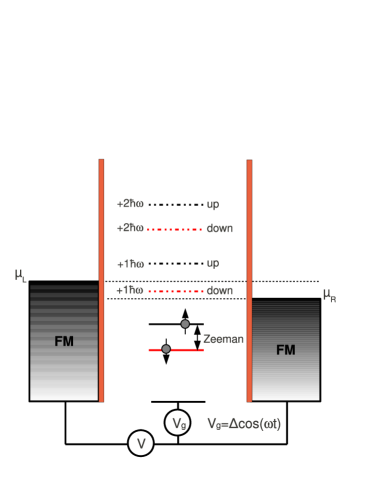
Figure 1: (color online) Energy diagram for the system considered. A quantum dot is coupled to a left and to a right ferromagnetic electron reservoirs via tunneling barriers. The dot level is Zeeman split. A capacitively coupled gate terminal introduces a periodic perturbation of the dot level. This modulation induces additional photon-assisted channels (dashed lines) for spin polarized transport.

II Model and theoretical formulation

For concreteness, the energy profile of our system is illustrated in Fig. 1 and is described by the Hamiltonian, $H=H_{L}+H_{R}+H_{D}(t)+H_{T}$, where

$$H_{L(R)}=\sum_{\mathbf{k}\sigma}\epsilon_{\mathbf{k}\sigma L(R)}c_{\mathbf{k}\sigma L(R)}^{\dagger}c_{\mathbf{k}\sigma L(R)},$$ (1)

describes the free electrons in the ($L$) or the right ($R$) lead, in which $c_{\mathbf{k}\sigma L(R)}$ [$c_{\mathbf{k}\sigma L(R)}^{\dagger}$] is the operator that annihilates [creates] an electrons in the lead $L(R)$ with momentum $\mathbf{k}$, spin $\sigma$ and energy $\epsilon_{\mathbf{k}\sigma L(R)}$. We consider a static source-drain applied voltage ($eV_{SD}=\mu_{L}-\mu_{R}$) which drives the system out of equilibrium, breaking the left/right symmetry of the Hamiltonian. The time dependence of our Hamiltonian is fully accounted via the dot Hamiltonian,

$$H_{D}(t)=\sum_{\sigma}\epsilon_{\sigma}(t)d_{\sigma}^{\dagger}d_{\sigma},$$ (2)

where $\epsilon_{\sigma}(t)=\epsilon_{d}(t)+\sigma E_{Z}/2$, with $\epsilon_{d}(t)$ being the time-dependent dot level and $E_{Z}$ a Zeeman splitting of the dot level due to an external magnetic field. Here we use $\sigma=+$ and $\sigma=-$ for spins up and down, respectively. The operator $d_{\sigma}$ ($d_{\sigma}^{\dagger}$) annihilates (creates) one electron with spin $\sigma$ and energy $\epsilon_{\sigma}(t)$ in the dot. In practice the time dependence in the dot level is controlled by an oscillating gate voltage $V_{g}(t)$, such that $\epsilon_{d}(t)=\epsilon_{0}+eV_{g}(t)$, where $\epsilon_{0}$ is the dc component of the energy and $eV_{g}(t)=\Delta\mathrm{cos}(\omega t)$ oscillates with amplitude $\Delta$ and frequency $\omega$. Finally

$$H_{T}=\sum_{\mathbf{k}\sigma\eta}(Vc_{\mathbf{k}\eta}^{\dagger}d_{\sigma}+V^{*}d_{\sigma}^{\dagger}c_{\mathbf{k}\sigma\eta}),$$ (3)

describes the tunnel coupling between the leads and the dot, with a constant coupling strength $V$ and allows for current to flow across the QD.

To calculate the time dependent spin polarized current we employ the Keldysh Green’s function formalismhh96 that allows for an appropriate approach to our nonequilibrium time-dependent situation. Starting from the current definition $I_{\sigma}^{\eta}(t)=-e\langle\dot{N}_{\sigma}\rangle=-ie\langle[H,N_{\sigma}]\rangle$, where $N_{\sigma}$ is the total number of particle operator for spin $\sigma$ (here we take $\hbar=1$), the current can be written asapj94

$$I^{\eta}_{\sigma}(t)=2e\mathrm{Re}\left\{\sum_{k}VG_{\sigma,k\sigma\eta}^{<}(t,t)\right\},$$ (4)

where $G_{\sigma,k\sigma\eta}^{<}(t,t^{\prime})=i\langle c_{k\sigma\eta}^{\dagger}(t^{\prime})d_{\sigma}(t)\rangle$. Using the equation of motion technique and taking analytical continuationhh96 to obtain $G_{\sigma,k\sigma\eta}^{<}(t,t^{\prime})$ one finds to the current the following

$$I^{\eta}_{\sigma}(t) = -2e\Gamma_{\eta}^{\sigma}\mathrm{Im}\Big{\{}\int\frac{d\epsilon}{2\pi}\int_{-\infty}^{t}dt_{1}e^{-i\epsilon(t_{1}-t)}$$ (5)

$$\phantom{xxxxxx}\times[G_{\sigma\sigma}^{r}(t,t_{1})f_{\eta}(\epsilon)+G_{\sigma\sigma}^{<}(t,t_{1})]\Big{\}},$$

where $f_{\eta}(\epsilon)$ is the Fermi distribution function of the $\eta$-th lead, and $\Gamma^{\eta}_{\sigma}=2\pi|V|^{2}\rho^{\eta}_{\sigma}$ gives the tunneling rate between lead $\eta$ and dot for spin component $\sigma$. $\rho^{\eta}_{\sigma}$ is the density of states for spin $\sigma$ in lead $\eta$. In the present model we assume constant density of states (wide-band limit). The ferromagnetism of the electrodes is modeled by considering $\Gamma_{\sigma}^{\eta}=\Gamma_{0}(1\pm p_{\eta})$ where $+$ ($-$) stands for spin up (down), $p_{\eta}$ is the polarization of lead $\eta$-thwr01 ; fms04 and $\Gamma_{0}$ the tunneling rate strength. The quantity $\Gamma_{0}$ is fixed along the paper, so all the other energies will be expressed in units of $\Gamma_{0}$. We consider both parallel (P) and antiparallel (AP) alignments of the lead polarizations. In the P case we assume majority down population in both leads, while in the AP configuration we take majority down population in the left lead and majority up population in the right lead. In terms of the parameters $p_{\eta}$ we have $p_{L}=p_{R}=p=-0.4$ for the P and $p_{L}=-p_{R}=p=-0.4$ for the AP case.commentnoncollinear

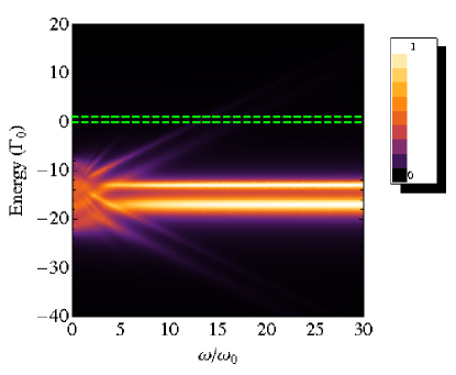
Figure 2: (color online) Color map of the total transmission coefficient $T(\epsilon,\omega)=T_{\uparrow}(\epsilon,\omega)+T_{\downarrow}(\epsilon,\omega)$ as a function of frequency and energy in the parallel alignment ($p_{L}=p_{R}=-0.4$). For increasing $\omega$, $T(\epsilon,\omega)$ develops additional photon-assisted peaks that allows off-resonant spin transport. The main two central peaks correspond to the Zeeman split levels $\epsilon_{\uparrow}^{0}=\epsilon_{0}+E_{Z}/2$ and $\epsilon_{\downarrow}^{0}=\epsilon_{0}-E_{Z}/2$. The satellite peaks are given by $\epsilon_{\uparrow}^{(n)}=\epsilon_{0}+E_{Z}/2\pm n\omega$ and $\epsilon_{\downarrow}^{(n)}=\epsilon_{0}-E_{Z}/2\pm n\omega$, with $n=1,2,3,...$. For increasing $\omega$, the satellite peaks tend to vanish and the system recovers its original two levels $\epsilon_{\uparrow}^{0}$ and $\epsilon_{\downarrow}^{0}$. The horizontal dashed lines delimit the conduction window [$\mu_{R},\mu_{L}$]. Units: Energy in units of $\Gamma_{0}$ and $\omega_{0}=\Gamma_{0}/\hbar$. Parameters: $\epsilon_{0}=-15\Gamma_{0}$, $E_{Z}=4\Gamma_{0}$, $\Delta=5\Gamma_{0}$, $\mu_{L}=1\Gamma_{0}$, $\mu_{R}=0$.

Taking the time average of the current we find

$$\langle I^{L}_{\sigma}(t)\rangle=-2e\frac{\Gamma_{\sigma}^{L}\Gamma_{\sigma}^{R}}{\Gamma_{\sigma}^{L}+\Gamma_{\sigma}^{R}}\int\frac{d\epsilon}{2\pi}[f_{L}(\epsilon)-f_{R}(\epsilon)]\mathrm{Im}\langle A_{\sigma}(\epsilon,t)\rangle,$$ (6)

where

$$\langle A_{\sigma}(\epsilon,t)\rangle=\sum_{n=-\infty}^{\infty}J_{n}^{2}(\frac{\Delta}{\omega})g_{n,\sigma}^{R}(\epsilon,\omega),$$ (7)

with $J_{n}$ being the n-th order Bessel function and $g_{n,\sigma}^{R}(\epsilon,\omega)=[\epsilon-\epsilon_{\sigma}^{0}-n\omega+i\frac{\Gamma_{\sigma}^{L}+\Gamma_{\sigma}^{R}}{2}]^{-1}$. Here we used the fact that $\epsilon_{\sigma}(t)=\epsilon_{\sigma}^{0}+\Delta\cos(\omega t)$, with $\epsilon_{\sigma}^{0}=\epsilon_{0}+\sigma E_{Z}/2$.

Substituting this result into Eq. (6), the current can be written in its Landauer formcommentreviewplatero

$$\langle I_{\sigma}^{L}(t)\rangle = e\int\frac{d\epsilon}{2\pi}T_{\sigma}(\epsilon)[f_{L}(\epsilon)-f_{R}(\epsilon)].$$

Here we define

$$T_{\sigma}(\epsilon)=\Gamma_{\sigma}^{L}\Gamma_{\sigma}^{R}\sum_{n=-\infty}^{\infty}\frac{J_{n}^{2}(\frac{\Delta}{\omega})}{(\epsilon-\epsilon_{\sigma}^{(n)})^{2}+(\frac{\Gamma_{\sigma}}{2})^{2}},$$ (9)

where $\epsilon_{\sigma}^{(n)}=\epsilon_{\sigma}^{0}+n\omega$. Eq. (9) shows that the harmonic modulation of the dot level yields to photon-assisted peaks in the transmission coefficient.gp04 In addition to this, here we have the spin splitting of these peaks and the ferromagnetic leads, that results in an enhanced spin photon-assisted transport.

A further simplification can be made in Eq. (II) by considering the low temperature regime, where the Fermi functions are approximated by step functions. In this regime, the integral in Eq. (II) is carried out in the range $[\mu_{L},\mu_{R}]$, thus resulting in

$$\langle I_{\sigma}^{L}\rangle=I_{\sigma}^{0}\Phi_{\sigma},$$ (10)

where $I_{\sigma}^{0}=e\frac{\Gamma_{\sigma}^{L}\Gamma_{\sigma}^{R}}{\Gamma_{\sigma}^{L}+\Gamma_{\sigma}^{R}}$ is the resonant current without modulated gate voltage and

$$\Phi_{\sigma}=\sum_{n=-\infty}^{\infty}J_{n}^{2}(\frac{\Delta}{\omega})[\Theta_{n}^{\sigma L}(\omega)-\Theta_{n}^{\sigma R}(\omega)]/\pi,$$ (11)

with $\Theta_{n}^{\sigma\eta}(\omega)=\arctan[2(\mu_{\eta}-\epsilon_{\sigma}^{0}-n\omega)/\Gamma_{\sigma}]$. In what follows we present our numerical results to the spin polarized transport.

III Numerical results

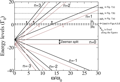
Figure 3: (color online) Multiplet structure developed in the presence of an oscillating gate frequency. The black lines correspond to spin up while the gray lines to spin down. The levels are shifted linearly with the gate frequency, following $\epsilon_{\sigma}^{(n)}=\epsilon_{\sigma}^{0}\pm n\omega$, $n=1,2,3,...$ The up and down levels are Zeeman split. The horizontal dashed lines correspond to the left ($\mu_{L}$) and to the right ($\mu_{R}$) chemical potentials. The channels $\epsilon_{\uparrow}^{(n)}$ and $\epsilon_{\downarrow}^{(n)}$ attain resonance within the conduction window $[\mu_{L},\mu_{R}]$ for certain frequencies, which differ for each spin component. Units: Energy levels in units of $\Gamma_{0}$ and $\omega_{0}=\Gamma_{0}/\hbar$. Parameters: $\epsilon_{0}=-15\Gamma_{0}$, $E_{Z}=4\Gamma_{0}$, $\Delta=5\Gamma_{0}$, $\mu_{L}=1\Gamma_{0}$, $\mu_{R}=0$.

Figure 2 shows the sum $T=T_{\uparrow}+T_{\downarrow}$ as a function of $\omega$ and energy in the case of polarized leads with parallel magnetizations. As $\omega$ increases, a multiplet structure takes place in the transmission coefficient [Eq. (9)]. The two central peaks in $T(\epsilon,\omega)$ correspond to $\epsilon_{\uparrow}^{0}$ and $\epsilon_{\downarrow}^{0}$, while the lateral peaks are related to $\epsilon_{\sigma}^{0}\pm n\omega$. Due to the Zeeman splitting, the whole pattern for $T_{\uparrow}$ is shifted upward while $T_{\downarrow}$ is moved downward. The highest of the peaks are strongly affected by the frequency. For the n-th peak its amplitude is given by $4\Gamma_{\sigma}^{L}\Gamma_{\sigma}^{R}J_{n}^{2}(\Delta/\omega)/\Gamma_{\sigma}^{2}$. For sufficiently large $\omega$, the additional photon-assisted peaks are suppressed, remaining only the two central peaks. The broadening difference for up and down spin channels comes from the ferromagnetism of the electrodes that are parallel aligned, with majority down population in both sides ($p_{L}=p_{R}=-0.4$). This gives rise to narrower spin up peaks than spin down ones. In the case of parallel aligned leads with majority up populations, we have basically the same structure, but with an inversion of the peak widths, with spin up peaks now becoming broader.

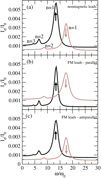
Figure 4: (color online) Spin resolved currents against gate frequency for leads (a) nonmagnetic and (b)-(c) ferromagnetic (black lines for spin up and gray lines for spin down). In panels (b) and (c) we show the parallel and antiparallel alignments, respectively. Both up and down currents show peaks corresponding to the crossing of $\epsilon_{\uparrow}^{(n)}$ and $\epsilon_{\downarrow}^{(n)}$ illustrated in Fig. (3). The highest peak for each spin component comes from the resonance of the levels $\epsilon_{\uparrow}^{(1)}$ and $\epsilon_{\downarrow}^{(1)}$, withing the conduction window. In the parallel alignment the majority down population in both leads turns into an amplification of the down current. In the antiparallel case, though, the currents are very similar to the nonmagnetic case. Units: $I_{0}=e\Gamma_{0}/\hbar$ and $\omega_{0}=\Gamma_{0}/\hbar$. Parameters: $\epsilon_{0}=-15\Gamma_{0}$, $E_{Z}=4\Gamma_{0}$, $\Delta=5\Gamma_{0}$, $\mu_{L}=1\Gamma_{0}$, $\mu_{R}=0$, $p=-0.4$.

Spin polarized transport can arise depending upon the position of the peaks of $T_{\sigma}(\epsilon,\omega)$ with respect to the conduction window. Fig. (3) shows the channels $\epsilon_{\uparrow}^{0}+n\omega$ and $\epsilon_{\downarrow}^{0}+n\omega$ for $n=0,\pm 1,\pm 2,\pm 3$ as black and gray lines, respectively. The left and right chemical potentials are indicated by the horizontal dashed lines. A net electron transport from the left to the right lead can take place whenever a channel $\epsilon_{\sigma}^{0}+n\omega$ attains the conduction window (CW) interval $[\mu_{L},\mu_{R}]$. Due to the Zeeman splitting, each spin component crosses $\mu_{L}$ or $\mu_{R}$ at different frequencies, thus resulting in a frequency selective spin transfer between the leads. In Fig. (3) we indicate by up and down arrows the corresponding crossing of the CW for spins $\uparrow$ and $\downarrow$, respectively. In the present study we focus on the off-resonant regime, where the dot levels $\epsilon_{\uparrow}^{0}$ and $\epsilon_{\downarrow}^{0}$ are below the CW. In this case only photon-assisted electrons can tunnel through the system. In order to match this condition we adopt to the numerical parameters the following values: $\epsilon_{0}=-15\Gamma_{0}$, $E_{Z}=4\Gamma_{0}$, $\Delta=5\Gamma_{0}$, $\mu_{L}=1\Gamma_{0}$ and $\mu_{R}=0$. Later on we will also look at distinct parameters in order to explore the robustness of our main results. In experiments we find typically $\Gamma_{0}\sim 100\mu eV$.dgg98_1 ; dgg98_2 ; fs99 So to the parameters assumed we have $E_{Z}\sim 400\mu eV$. This Zeeman energy split is reasonable for semiconductor quantum dots in the presence of magnetic fields $\sim$ 1-10 T.rh03 Additionally, for these values we find $\omega_{0}=\frac{\Gamma_{0}}{\hbar}\sim 150$ GHz. So the present theoretical effects could be observed for gate frequencies around 1.5 THz [$\omega\sim 10\omega_{0}$, see Fig. (4)].thzelectronics Alternatively, if $\Gamma_{0}$ is reduced to $\sim 1\mu$eV,sami ; km07 we obtain gate frequencies around $\omega\sim 10\omega_{0}\sim 15$ GHz, which is quite feasible experimentally.he10 Our currents will be given in units of $I_{0}=e\Gamma_{0}/\hbar$, which is in the range $I_{0}\sim$ 0.24nA-24nA for $\Gamma_{0}\sim 1\mu$eV - 100 $\mu$eV. Since our spin resolved photon-assisted currents are typically $\sim 10^{-3}I_{0}$, we have pA currents, which could be measured with picoampere measurement technologies.

Comparing Fig. (3) to Fig. (2) one can note that even though $n=3$ and $n=2$ attain resonance withing $[\mu_{L},\mu_{R}]$, their corresponding transmission amplitude are very low, which makes the transport weak via those channels. In contrast, the $n=1$ channels, for up and down spins, have a higher transmission amplitude, which makes the spin transfer via these channels more appreciable.

Fig. (4) shows the up and down components of the current against gate frequency. Three cases are considered: (a) nonmagnetic leads, ferromagnetic leads in the (b) parallel and (c) antiparallel alignments. In all the three cases two major peaks are found ($n=1$). Satellite peaks for high order channels ($n=2,3$) are also seen. Each peak emerges whenever a channel $\epsilon_{\sigma}^{0}+n\omega$ enters the conduction window [indicated by $\uparrow$ and $\downarrow$ arrows in Fig. (3)]. Due to the Zeeman splitting, the resonance for spin up arises in lower frequencies than that for spin down. Additionally, the interplay between Zeeman splitting and the amplitude of the transmission coefficient results into a higher peak for spin up than for spin down in the case of nonmagnetic leads.commentotherwork Further amplification of the spin down current peak is observed when the leads are made ferromagnetic. In Fig. 4(b) we present $I_{\uparrow}$ and $I_{\downarrow}$ for leads parallel aligned, with a majority down population in both sides. This means that we assume for the polarization parameter a negative value, with $p_{L}=p_{R}=p=-0.4$. This implies that $\Gamma_{\downarrow}^{L,R}>\Gamma_{\uparrow}^{L,R}$ ($\rho_{\downarrow}^{L,R}>\rho_{\uparrow}^{L,R}$), which favors more the spin down electrons to tunnel through the system, thus increasing the spin down current peak. In the antiparallel case, where we have a majority down population in the left lead and a majority up population in the right lead ($\Gamma_{\downarrow}^{L}>\Gamma_{\uparrow}^{L}$ and $\Gamma_{\downarrow}^{R}<\Gamma_{\uparrow}^{R}$ for $p_{L}=-p_{R}=p=-0.4$), the incoming and outgoing rates compensate each other. This results into equal weights for both up and down currents, so the current remains almost the same compared to the nonmagnetic case.

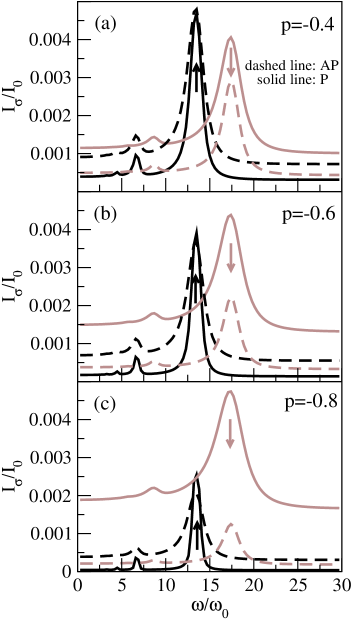
Figure 5: (color online) Spin resolved currents against gate frequency for different polarization $p$, in both parallel and antiparallel configurations (black lines for spin up and gray lines for spin down). In the plots $p$ is negative, which means that both leads have majority spin down population in the P case and majority down (up) population in the left (right) lead for the AP case. In the P alignment when $p$ increases (in modulus) the tunneling rates between the dot and the leads enlarge for spin down and reduce for spin up. This results in an amplification of $I_{\downarrow}$ and a suppression of $I_{\uparrow}$ as observed. In the AP alignment both $I_{\uparrow}$ and $I_{\downarrow}$ are suppressed as $|p|$ increases. Units: $I_{0}=e\Gamma_{0}/\hbar$ and $\omega_{0}=\Gamma_{0}/\hbar$. Parameters: $\epsilon_{0}=-15\Gamma_{0}$, $E_{Z}=4\Gamma_{0}$, $\Delta=5\Gamma_{0}$, $\mu_{L}=1\Gamma_{0}$, $\mu_{R}=0$.

Fig. (5) shows how the spin resolved currents evolve when the leads polarizations are enlarged in both P and AP configurations. When $p$ becomes more negative, the spin down tunneling rates $\Gamma_{\downarrow}^{L}$ and $\Gamma_{\downarrow}^{R}$ are strengthened, while $\Gamma_{\uparrow}^{L}$ and $\Gamma_{\uparrow}^{R}$ are diminished in the parallel case. This amplifies the peak for spin down current while suppresses the peak for spin up, thus making the current more down polarized. Eventually, for larger enough $|p|$ the $I_{\downarrow}$ current dominates over $I_{\uparrow}$ for all gate frequencies, Conversely, in the antiparallel configuration, as $p$ becomes more negative, both $I_{\uparrow}$ and $I_{\downarrow}$ are suppressed. One may note that when we pass from P to AP alignment, the major spin up peak has its width broadened. This can also be seen by calculating the width of this peak: $\Gamma_{\uparrow}=\Gamma_{\uparrow}^{L}+\Gamma_{\uparrow}^{R}=2\Gamma_{0}(1-|p|)$ and $\Gamma_{\uparrow}=\Gamma_{\uparrow}^{L}+\Gamma_{\uparrow}^{R}=2\Gamma_{0}$ for P and AP, respectively. In particular, this broadening effect makes the total antiparallel current slightly higher than the parallel current ($I^{P}<I^{AP}$), and this results into a negative magnetoresistance, as we will see next.

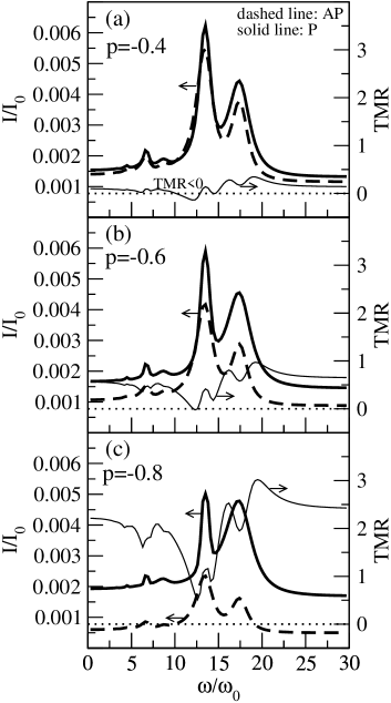
Figure 6: Total current ($I_{\uparrow}+I_{\downarrow}$) in both P and AP alignment and TMR as a function of the gate frequency. From panels (a) to (c) the left and right leads polarization are enlarged ($p=-0.4$, $-0.6$, $-0.8$). The highest current peak is predominantly due to spin up transport while the second highest peak is more spin down like. The TMR tends to be suppressed or amplified around the spin up or spin down peaks, respectively. In particular, the TMR attains negative values for $p=-0.4$ in a short gate frequency range, due to a photon-assisted inversion of the spin valve effect ($I^{P}<I^{AP}$). Units: $I_{0}=e\Gamma_{0}/\hbar$ and $\omega_{0}=\Gamma_{0}/\hbar$. Parameters: $\epsilon_{0}=-15\Gamma_{0}$, $E_{Z}=4\Gamma_{0}$, $\Delta=5\Gamma_{0}$, $\mu_{L}=1\Gamma_{0}$, $\mu_{R}=0$.

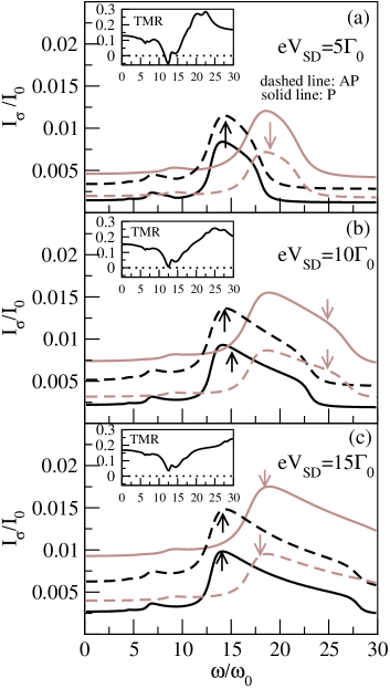
Figure 7: (color online) Spin resolved currents against gate frequency for both parallel and antiparallel configurations (black lines for spin up and gray lines for spin down). From panels (a) to (c) we increase the bias voltage [(a) $eV_{SD}=5\Gamma_{0}$, (b) $eV_{SD}=10\Gamma_{0}$, (c) $eV_{SD}=15\Gamma_{0}$], thus enlarging the conduction window [dashed lines in Fig. 3]. Fig. 7(a) is similar to Fig. 5(a), except by the width of the peaks that are slightly enlarged by the CW. When $eV_{SD}$ increases even further [panels (b)-(c)] the peaks turn even more broaden. In the insets we show the TMR for each bias voltage. For $eV_{SD}=5\Gamma_{0}$ the TMR presents a negative value around $\omega\approx 12.5\omega_{0}$. For $eV_{SD}=10\Gamma_{0}$ and $eV_{SD}=15\Gamma_{0}$ the TMR becomes positive for all frequencies. Units: $I_{0}=e\Gamma_{0}/\hbar$ and $\omega_{0}=\Gamma_{0}/\hbar$. Parameters: $\epsilon_{0}=-15\Gamma_{0}$, $E_{Z}=4\Gamma_{0}$, $\Delta=5\Gamma_{0}$, $\mu_{L}-\mu_{R}=eV_{SD}$, $p=-0.4$.

In Fig. (6) we show the total current in both P and AP alignment and the tunnel magnetoresistance, defined according to

$$TMR=\frac{I^{P}-I^{AP}}{I^{AP}},$$ (12)

where $I^{P/AP}=I^{P/AP}_{\uparrow}+I^{P/AP}_{\downarrow}$. The highest current peak is related to the resonance of the channel $\epsilon_{\uparrow}^{(1)}$ with the CW. The second highest peak is due to spin down resonance, $\epsilon_{\downarrow}^{(1)}\approx\mu_{R}$. The spin valve effect is clearly seen for almost all frequencies, i.e., $I^{P}>I^{AP}$. However, for frequencies around 10$\omega_{0}$, we observe $I^{P}<I^{AP}$ for $p=-0.4$ [Fig. 6(a)]. This photon-assisted opposite spin valve effect is related to the broadening of the spin up peak discussed in Fig. (5), when the lead polarizations rotate from P to AP alignment. This feature is reflected in the TMR, which acquires negative values. Notice that near the position of the spin up peak the TMR is fully suppressed, while near to the peak of the spin down current it is enlarged for all values of $p$. This indicates that the magnetoresistance is mainly dominated by spin down transport.

Since from the experimental point of view the quantities $V_{SD}$, $\epsilon_{d}$ and $E_{Z}$ are relative easily tunable experimental parameters, we analyze how these quantities affect the present results, aiming to providing a better guide for future experimental realizations. For instance, using the same set of parameters adopted previously [$p_{L}=-0.4$, $p_{R}=-0.4$(P), $p_{R}=+0.4$(AP), $\epsilon_{0}=-15\Gamma_{0}$, $\Delta=5\Gamma_{0}$, $E_{Z}=4\Gamma_{0}$], in Fig. (7) we show how the spin resolved currents evolve when the source-drain voltage increases in both parallel and antiparallel configurations. The bias voltages considered are (a) $eV_{SD}=5\Gamma_{0}$, (b) $10\Gamma_{0}$ and (c) $15\Gamma_{0}$. These values were also indicated by dashed lines in Fig. (3). By comparing Fig. 7(a) to Fig. 5(a) one can note that the peaks are broadened as $V_{SD}$ increases. This feature can be understood looking at the different conduction windows (dashed lines) in Fig. (3). As $\mu_{L}-\mu_{R}$ becomes larger, the frequency range in which the photon-assisted channels remains inside the CW becomes wider. In the insets of Fig. (7) we show the TMR against frequency for each $V_{SD}$ considered. Notice that for $eV_{SD}=10\Gamma_{0}$ and $eV_{SD}=15\Gamma_{0}$ [panels (b) and (c), respectively] the TMR is positive for all frequencies.

In order to obtain a clear picture on the set of parameters needed to obtain a negative TMR, in Fig. (8) we plot in a color map of the total transmission coefficient difference, $\Delta T=T^{P}-T^{AP}$, against gate frequency (horizontal axis) and energy $\epsilon$ (vertical axis), for two different Zeeman splitting energies: (a) $E_{Z}=4\Gamma_{0}$ and (b) $E_{Z}=8\Gamma_{0}$. Notice the appearance of negative values (dark regions) around the spin up peaks, when the up and down branches are not overlapping. The overlap can be avoided by controlling the Zeeman splitting. Observe that for $E_{Z}=8\Gamma_{0}$ [panel (b)] the spin up and spin down branches are far enough from each other to ensure relatively large dark areas. This effect can be understood in terms of the broadening of the photon-assisted peaks. In the P configuration, the spin down peaks at the transmission coefficient are broader than the spin up ones, as can be seen by the rates $\Gamma_{\downarrow}=\Gamma_{\downarrow}^{L}+\Gamma_{\downarrow}^{R}=2\Gamma_{0}(1+|p|)=2.8\Gamma_{0}$ and $\Gamma_{\uparrow}=2\Gamma_{0}(1-|p|)=1.2\Gamma_{0}$ ($|p|=0.4$). So when these peaks coincide at the same energy ($E_{Z}=0$) the spin down peaks lie above the spin up ones, thus making the total transmission coefficient dominated by the spin down component. When the magnetic alignment is rotated from P to AP, the width of the spin up peak increases and spin down diminishes, becoming both $2\Gamma_{0}$. This facilitates $T_{\uparrow}^{AP}>T_{\uparrow}^{P}$ and $T_{\downarrow}^{AP}<T_{\downarrow}^{P}$ nearby each transmission peak. If the peaks are far enough from each other ($E_{Z}\neq 0$) it is possible to obtain $T=T_{\uparrow}+T_{\downarrow}\approx T_{\uparrow}$ around the up peaks, leading to $T^{AP}\approx T_{\uparrow}^{AP}>T^{P}\approx T_{\uparrow}^{P}$ [see Fig. 9(c) for clarity]. This is the main condition for a negative TMR.commentmajorityup

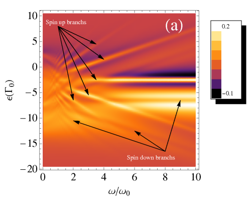
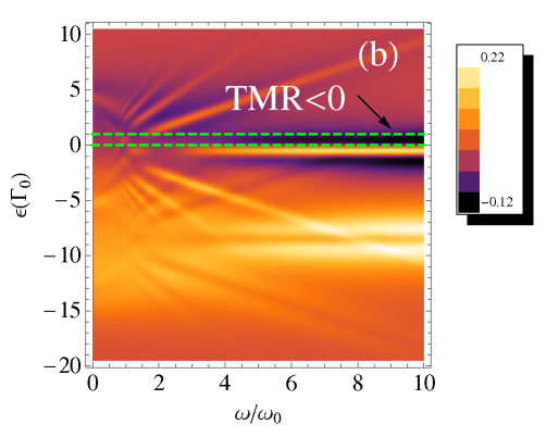
Figure 8: (color online) Two-dimensional map of the difference $\Delta T=T^{P}-T^{AP}$ against frequency $\omega$ and $\epsilon$ for two different Zeeman splitting: (a) $E_{Z}=4\Gamma_{0}$ and (b) $E_{Z}=8\Gamma_{0}$. The dark regions indicate $T^{AP}>T^{P}$ which results in negative TMR. As $E_{Z}$ increases [from panel (a) to (b)] the dark ares enlarge. This is so because the spin up and down channels become apart from each other, allowing to have $T^{AP}=T_{\uparrow}^{AP}+T_{\downarrow}^{AP}\approx T_{\uparrow}^{AP}>T^{P}=T_{\uparrow}^{P}+T_{\downarrow}^{P}\approx T_{\uparrow}^{P}$ (broadening effect) around the spin up channels. By playing with the set of parameters one can place the conduction window of the system in the darker region of the map, which results into a more negative TMR. Units: $I_{0}=e\Gamma_{0}/\hbar$ and $\omega_{0}=\Gamma_{0}/\hbar$. Parameters: $\epsilon_{0}=-4.5\Gamma_{0}$, $\Delta=5\Gamma_{0}$, $\mu_{L}=1\Gamma_{0}$, $\mu_{R}=0$, $p=-0.4$.

For instance, by tunning the set of parameters such that the CW lies on the darker area of the map, the TMR becomes negative. By increasing the CW, we can eventually cover an energy range with more bright than dark areas, resulting in a positive TMR.

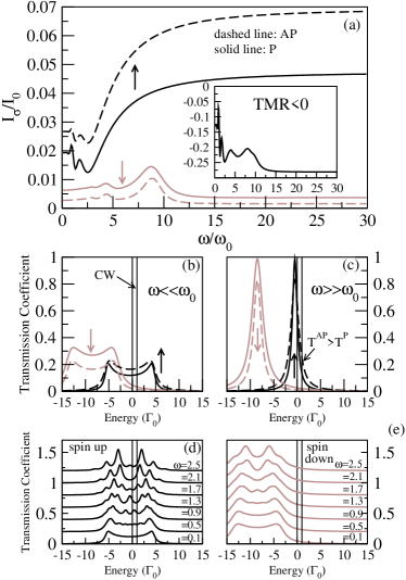
Figure 9: (color online) (a) Spin resolved currents in both P and AP alignments against gate frequency for the conduction window drawn in Fig. 8(b). Similar to previous figures, the spin down component reveals peaks at some particular frequencies due to the matches $\epsilon_{\sigma}^{(n)}=\mu_{R}$. In contrast, the spin up current oscillates and then it tends to a relatively large saturation value for large $\omega$. In the inset of Fig. 9(a) we show the TMR which acquires negative values in accordance to the CW in Fig. 8(b). Panels (b)-(c) present the spin resolved transmission coefficient for (b) small and (c) large $\omega$ in both P and AP configurations. The thin vertical lines denote the border of the CW. In particular, observe in panel (c) that inside the CW we have $T_{\uparrow}^{AP}>T_{\uparrow}^{P}$. Since $T_{\downarrow}^{P/AP}$ is too small at the CW, the total transmission coefficient $T^{P/AP}$ is given essentially by $T_{\uparrow}^{P/AP}$, so $T^{AP}=T^{AP}_{\uparrow}+T^{AP}_{\downarrow}\approx T^{AP}_{\uparrow}>T^{P}=T^{P}_{\uparrow}+T^{P}_{\downarrow}\approx T^{P}_{\uparrow}$ around the peak. This results in a negative TMR. In panels (d)-(e) we plot (d) $T_{\uparrow}^{P}$ and (e) $T_{\downarrow}^{P}$ for different values of $\omega$. The curves were vertically displaced for clarity. As $\omega$ increases additional peaks emerge mainly in the interval $\epsilon_{\sigma}^{0}\pm\Delta=\epsilon_{\sigma}^{0}\pm 5\Gamma_{0}$. More specifically, in the spin up case the appearance and suppression of these additional peaks inside the CW gives rise to the oscillatory patter of $I_{\uparrow}$ in the low frequency limit. Units: $I_{0}=e\Gamma_{0}/\hbar$ and $\omega_{0}=\Gamma_{0}/\hbar$. Parameters: $\epsilon_{0}=-4.5\Gamma_{0}$, $E_{Z}=8\Gamma_{0}$, $\Delta=5\Gamma_{0}$, $\mu_{L}=1\Gamma_{0}$, $\mu_{R}=0$, $p=-0.4$.

In Fig. (9) we show the current vs. $\omega$ obtained for the conduction window set as in Fig. 8(b)[dashed (green) lines] Since the CW is dominated by a dark region ($T^{P}<T^{AP}$) we expect $TMR<0$. The spin up and spin down currents in Fig. 9(a) reveal contrasting behavior. While the spin down current shows the same behavior already seen in previous results [e.g., Fig. (5)], the spin up current oscillates and then it increases to a higher saturation value. This higher value of $I_{\uparrow}$ in the large frequency limit can be understood by looking at the transmission coefficient in panels 9(b) and (c). Spin up and spin down transmissions coefficients are drawn in both P and AP configurations. The vertical thin solid lines give the border of the CW. Comparing the amplitude of $T_{\uparrow}$ inside the CW for both $\omega\ll\omega_{0}$ and $\omega\gg\omega_{0}$, we observe that $T_{\uparrow}$ becomes amplified for larger frequencies, which results into higher spin up current in this limit. Conversely, the spin down transmission coefficient is slightly higher in the CW for $\omega\ll\omega_{0}$, resulting in a spin down current a bit higher in the low frequency limit, compared to its value in the high frequency regime.

To better understand the oscillatory structure found in the spin up current, we plot in Fig. 9(d) the spin up parallel transmission coefficient $T_{\uparrow}^{P}$ vs. energy for various $\omega$. As $\omega$ increases the transmission coefficient develops a variety of peaks mainly in the range between $\epsilon_{\uparrow}^{0}-5\Gamma_{0}$ and $\epsilon_{\uparrow}^{0}+5\Gamma_{0}$ ($\epsilon^{0}_{\uparrow}\pm\Delta$). Since this energy interval contains the CW, some of the photon-assisted peaks that arise for increasing $\omega$ appear within the CW and eventually lie outside it for large enough $\omega$, followed by a new peak emerging inside it. This results in an oscillatory pattern of the current. In panel 9(e) we show $T_{\downarrow}^{P}$ as function of energy for the same values of $\omega$ as in panel (d). Since $\epsilon^{0}_{\downarrow}+\Delta<\mu_{R}$ the photon-assisted peaks can only cross the CW for particular frequencies, which gives rise to the peaks observed. Finally, in the inset of Fig. 9(a) we plot the TMR, which presents very low negative values ($\sim-30$%). This negative TMR is a result of the set of parameters chosen from Fig. 8.

IV Conclusion

We have studied spin polarized transport in a quantum dot attached to ferromagnetic leads in the presence of an oscillating gate voltage $V_{g}(t)$. A static source-drain bias voltage is also applied in order to generate current. The oscillating $V_{g}(t)$ gives rise to photon-assisted transport channels that allow electrons to flow through the system. Due to a Zeeman splitting of the dot level, the photon-assisted contributions to the transport are distinct for spins up and down, providing an interesting way to obtain current polarization that can be controlled by gate frequency. As the leads polarization is enlarged, with a majority down population in both leads (P alignment), the spin down photon-assisted current peak is enhanced, while the spin up peak is suppressed. Moreover, when the relative polarization alignment of the leads is switched from P to AP, the width of the main spin up peak of the current is broadened. This additional broadening effect results in an opposite spin valve behavior ($I^{P}<I^{AP}$) for gate frequencies around the spin up resonance. As a result, a photon-assisted negative tunnel magnetoresistance is found.

References

- (1) N. S. Wingreen, A. P. Jauho, and Y. Meir, Phys. Rev. B 48, 8487 (1993).
- (2) L. J. Geerligs, V. F. Anderegg, P. A. M. Holweg, J. E. Mooij, H. Pothier, D. Esteve, C. Urbina, M. H. Devoret, Phys. Rev. Lett. 64, 2691 (1990).
- (3) L. P. Kouwenhoven, A. T. Johnson, N. C. van der Vaart, C. J. P. M. Harmans, C. T. Foxon, Phys. Rev. Lett. 67, 1626 (1991).
- (4) C. Bruder and H. Schoeller, Phys. Rev. Lett. 72, 1076 (1994).
- (5) L. P. Kouwenhoven, S. Jauhar, K. McCormick, D. Dixon, P. L. McEuen, Yu. V. Nazarov, N. C. van der Vaart, and C. T. Foxon, Phys. Rev. B 50, 2019(R) (1994).
- (6) L. P. Kouwenhoven, S. Jauhar, J. Orenstein, P. L. McEuen, Y. Nagamune, J. Motohisa, and H. Sakaki, Phys. Rev. Lett. 73, 3443 (1994).
- (7) B. J. Keay, S. J. Allen, Jr., J. Galán, J. P. Kaminski, K. L. Campman, A. C. Gossard, U. Bhattacharya, and M. J. W. Rodwell, Phys. Rev. Lett. 75, 4098 (1995).
- (8) For a review see G. Platero and R. Aguado, Phys. Rep. 395, 1 (2004).
- (9) C. A. Stafford and N. S. Wingreen, Phys. Rev. Lett. 76, 1916 (1996).
- (10) A. F. Amin, G. Q. Li, A. H. Phillips, and U. Kleinekathöfer, Eur. Phys. J. B 68, 103 (2009).
- (11) F. Cavaliere, M. Governale, and J. König, Phys. Rev. Lett. 103, 136801 (2009).
- (12) R. Zhu and H. Chen, Appl. Phys. Lett. 95, 122111 (2009).
- (13) E. Prada, P. San-Jose, and H. Schomerus, Phys. Rev. B 80, 245414 (2009).
- (14) G. M. M. Wakker and M. Blaauboer, Phys. Rev. B 82, 205432 (2010).
- (15) M. Alos-Palop and M. Blaauboer, arXiv: 1102.0926 (2011).
- (16) J. Splettstoesser, M. Governale, J. König, and M. Büttiker, Phys. Rev. B 81, 165318 (2010).
- (17) S. Kurth, G. Stefanucci, E. Khosravi, C. Verdozzi, and E. K. U. Gross, Phys. Rev. Lett. 104, 236801 (2010).
- (18) G. A. Prinz, Science 282, 1660 (1998); S. A. Wolf, D. D. Awschalom, R. A. Buhrman, J. M. Daughton, S. von Molnár, M. L. Roukes, A. Y. Chtchelkanova, and D. M. Treger, ibid. 294, 1488 (2001); Semiconductor Spintronics and Quantum Computation, edited by D. Awschalom, D. Loss, and N. Samarth (Springer, Berlin 2002); D. D. Awschalom and M. E. Flatté, Nat. Phys. 3, 153 (2007).
- (19) E. Cota, R. Aguado, and G. Platero, Phys. Rev. Lett. 94, 107202 (2005).
- (20) R. Sánchez, E. Cota, R. Aguado, and G. Platero, Phys. Rev. B 74, 035326 (2006); R. Sánchez, E. Cota, R. Aguado, and G. Platero, Physica E 34, 405 (2006).
- (21) E. R. Mucciolo, C. Chamon, and C. M. Marcus, Phys. Rev. Lett. 89, 146802 (2002).
- (22) T. Aono, Phys. Rev. B 67 155303 (2003).
- (23) S. K. Watson, R. M. Potok, C. M. Marcus, and V. Umansky, Phys. Rev. Lett. 91, 258301 (2003).
- (24) F. M. Souza, Phys. Rev. B 76, 205315 (2007).
- (25) E. Perfetto, G. Stefanucci, and M. Cini, Phys. Rev. B 78, 155301 (2008).
- (26) P. Trocha, Phys. Rev. B 82, 115320 (2010).
- (27) F. M. Souza, S. A. Leão, R. M. Gester, and A. P. Jauho, Phys. Rev. B 76, 125318 (2007).
- (28) F. M. Souza and J. A. Gomez, Phys. Status Solid B 246, 431 (2009).
- (29) R. Hanson and D. D. Awschalom, Nature 453, 1043 (2008).
- (30) J. M. Elzerman, R. Hanson, L. H. W. van Beveren, B. Witkamp, L. M. K. Vandersypen, and L. P. Kouwenhoven, Nature 430, 431 (2004).
- (31) R. Hanson, L. H. W. van Beveren, I. T. Vink, J. M. Elzerman, W. J. M. Naber, F. H. L. Koppens, L. P. Kouwenhoven, and L. M. K. Vandersypen, Phys. Rev. Lett. 94, 196802 (2005).
- (32) A. C. Johnson, J. R. Petta, J. M. Taylor, A. Yacoby, M. D. Lukin, C. M. Marcus, M. P. Hanson, and A. C. Gossard, Nature 435 925 (2005).
- (33) J. R. Petta, A. C. Johnson, J. M. Taylor, E. A. Laird, A. Yacoby, M. D. Lukin, C. M. Marcus, M. P. Hanson, A. C. Gossard, Science 309, 2180 (2005).
- (34) F. H. L. Koppens, C. Buizert, K. J. Tielrooij, I. T. Vink, K. C. Nowack, T. Meunier, L. P. Kouwenhoven, and L. M. K. Vandersypen, Nature 442, 766 (2006).
- (35) C. Barthel, J. Medford, C. M. Marcus, M. P. Hanson, and A. C. Gossard, Phys. Rev. Lett. 105, 266808 (2010).
- (36) H. Haug and A. P. Jauho, Quantum Kinetics in Transport and Optics of Semiconductors, Springer Solid-State Sciences 123 (1996).
- (37) In the present calculation we follow the formulation developed in A. P. Jauho, N. S. Wingreen, and Y. Meir, Phys. Rev. B 50, 5528 (1994).
- (38) W. Rudziński and J. Barnaś, Phys. Rev. B 64, 85318 (2001).
- (39) F. M. Souza, J. C. Egues, and A. P. Jauho, Braz. J. Phys. 34, 565 (2004).
- (40) In the present work we consider only the P and AP alignments. We expect that for more general non-collinear magnetizations the present currents will vary monotonically from their parallel () to their antiparallel () values. In the adiabatic-pumping regime it was found (see, for instance, Ref. [js08, ]) a monotonic suppression of the pumped charge as the angle between the magnetizations of the left and right leads is continuously varied from to .
- (41) J. Splettstoesser, M. Governale, and J. König, Phys. Rev. B 77 195320 (2008).
- (42) An alternative but equivalent version of this equation was derived in Ref. [gp04, ], where the distinction between this result and the Tien-Gordon formula was discussed.
- (43) D. G.-Gordon, H. Shtrikman, D. Mahalu, D. A.-Magder, U. Meirav, M. A. Kastner, Nature 391, 156 (1998).
- (44) D. Goldhaber-Gordon, J. Göres, M. A. Kastner, H. Shtrikman, D. Mahalu, and U. Meirav, Phys. Rev. Lett. 81, 5225 (1998).
- (45) F. Simmel, R. H. Blick, J. P. Kotthaus, W. Wegscheider, and M. Bichler, Phys. Rev. Lett. 83, 804 (1999).
- (46) R. Hanson, B. Witkamp, L. M. K. Vandersypen, L. H. Willems van Beveren, J. M. Elzerman, and L. P. Kouwenhoven, Phys. Rev. Lett. 91, 196802 (2003).
- (47) Significant improvements on THz electronics have been recently achieved. See for instance, T. W. Crowe, W. L. Bishop, D. W. Porterfield, J. L. Hesler, R. M. Weikle, IEEE J. Solid-State Circuits, 40 2104 (2005).
- (48) S. Amasha (private communication).
- (49) K. MacLean, S. Amasha, I. P. Radu, D. M. Zumbühl, M. A. Kastner, M. P. Hanson, and A. C. Gossard, Phys. Rev. Lett. 98, 036802 (2007).
- (50) H. Eisele, S. P. Khanna, and E. H. Linfield, Appl. Phys. Lett. 96 072101 (2010).
- (51) Two split peaks in a pumping current, one peak for each spin component, were also found by Cota et al. in Ref. [ec05, ] for a double dot system in the presence of magnetic field.
- (52) In the case of majority up population in both leads in the P alignment, we have the opposite behavior seen in Fig. (8), i.e., the maxima become minima and vice-versa. So the dark areas in the plot () arise around the spin down branches, instead of the spin up ones.