Multiwavelength Observations of the Gamma-Ray Blazar PKS 0528+134 in Quiescence

Abstract

We present multiwavelength observations of the ultraluminous blazar-type radio loud quasar PKS 0528+134 in quiescence during the period July to December 2009. Four Target-of-Opportunity (ToO) observations with the XMM-Newton Satellite in the 0.2 – 10 keV range were supplemented with optical observations at the MDM Observatory, radio and optical data from the GLAST-AGILE Support Program (GASP) of the Whole Earth Blazar Telescope (WEBT) and the Very Long Baseline Array (VLBA), additional X-ray data from the Rossi X-ray Timing Explorer (RXTE; 2 – 10 keV) and from Suzaku (0.5 – 10 keV) as well as $\gamma$-ray data from the Fermi Large Area Telescope (LAT) in the 100 MeV – 200 GeV range. In addition, publically available data from the SMARTS blazar monitoring program and the University of Arizona / Steward Observatory Fermi Support program were included in our analysis.

We found no evidence of significant flux or spectral variability in $\gamma$-rays and most radio bands. However, significant flux variability on a time scale of several hours was found in the optical regime, accompanied by a weak trend of spectral softening with increasing flux. We suggest that this might be the signature of a contribution of unbeamed emission, possibly from the accretion disk, at the blue end of the optical spectrum. The optical flux is weakly polarized with rapid variations of the degree and direction of polarization, while the polarization of the 43 GHz radio core remains steady, perpendicular to the jet direction. Optical spectropolarimetry of the object in the quiescent state suggests a trend of increasing degree of polarization with increasing wavelength, providing additional evidence for an unpolarized emission component, possibly thermal emission from the accretion disk, contributing towards the blue end of the optical spectrum. Over an extended period of several months, PKS 0528+134 shows moderate (amplitude $\lesssim 50$ %) flux variability in the X-rays and most radio frequencies on $\sim 1$ – 2 week time scales. We constructed four spectral energy distributions (SEDs) corresponding to the times of the XMM-Newton observations. We find that even in the quiescent state, the bolometric luminosity of PKS 0528+134 is dominated by its $\gamma$-ray emission.

A leptonic single-zone jet model produced acceptable fits to the SEDs with contributions to the high-energy emission from both synchrotron self-Compton radiation and Comptonization of direct accretion disk emission. Fit parameters close to equipartition between the energy densities of the magnetic field and the relativistic electron population were obtained. The moderate variability on long time scales, compared to expected radiative cooling time scales, implies the existence of on-going particle acceleration, while the observed optical polarization variability seems to point towards a turbulent acceleration process. Turbulent particle acceleration at stationary features along the jet therefore appears to be a viable possibility for the quiescent state of PKS 0528+134.

1 Introduction

Blazars (BL Lac objects and gamma-ray loud flat spectrum radio quasars [FSRQ]) are the most extreme type of active galactic nuclei (AGN). They were historically defined through extreme flux variability throughout the electromagnetic spectrum, and sometimes strong and variable linear polarization at radio and optical wavelengths. In the 1990s, observations by EGRET on board the Compton Gamma-Ray Observatory revealed large $\gamma$-ray fluxes (often dominating the bolometric luminosity of the source) from many blazars. The radio through optical emission from blazars is commonly interpreted as synchrotron emission from ultrarelativistic electrons in a relativistic plasma jet that is closely aligned with our line of sight ($\theta_{obs}<20^{\arcdeg}$). This assertion is supported by the superluminal motion that most blazars exhibit (e.g., Jorstad et al., 2001; Lister et al., 2009; Piner et al., 2006) as well as by the observed luminosity and variability timescales observed in these objects. In extreme cases, variability time scales down to a few minutes have been found in the very high energy (VHE) $\gamma$-ray regime (e.g., Albert et al., 2007; Aharonian et al., 2007).

Two competing classes of models are currently being considered for the origin of the high-energy (X-ray through $\gamma$-ray) emission from blazars. In leptonic models, hadrons (primarily protons) in the jet (if present in substantial numbers at all), are assumed not to be accelerated to ultrarelativistic energies. They do not exceed the threshold for photo-pion production processes on the low-frequency radiation field in the jet, and proton synchrotron radiation is assumed to be negligible. Therefore, in leptonic models, the high-energy radiative output is dominated by Compton scattering of low-frequency photons off relativistic electrons. In hadronic models, it is assumed that ultrarelativistic protons exist in sufficient number. In such a scenario, the protons will dominate the radiative output via proton synchrotron radiation and synchrotron and Compton emission from secondary particles. Those are produced in photo-pion production and subsequent pion and muon decay and electromagnetic cascade processes. For a recent review of blazar emission models, see, e.g., Böttcher (2010).

The mechanism(s) of acceleration of particles to ultrarelativistic energies in blazar jets are currently very poorly understood. Particle acceleration may be related to relativistic shocks in an unsteady flow (e.g., Marscher & Gear, 1985), internal shocks resulting from the collision of relativistic plasma blobs ejected at different speeds (e.g., Spada et al., 2001; Mimica et al., 2004; Joshi & Böttcher, 2010; Böttcher & Dermer, 2010), re-collimation shocks (e.g., Bromberg & Levinson, 2009), or relativistic shear layers in radially stratified jets (e.g., Stawarz & Ostrowski, 2002; Rieger & Duffy, 2004, 2006), to name just a few plausible scenarios. Signatures that reveal the nature of particle acceleration in blazar jets may be found both in spectral and variability features. The nature of the acceleration mechanism is reflected in the shape of the produced particle spectra. Those, in turn, can be inferred from the shape of the non-thermal photon spectra, in particular in the synchrotron part of the SED (e.g., Finke et al., 2008). The dynamics and light travel time effects, in particular in shock acceleration scenarios, will leave distinct imprints in the observed variability features (e.g., Böttcher & Dermer, 2010).

Observational studies of blazars have so far mostly focused on bright, flaring states of blazars. This is the consequence of observational constraints which make detailed measurements of spectral and variability features in X-rays and $\gamma$-rays difficult in low flux states. However, blazars are known to spend most of the time in their quiescent state which has so far received very little attention and is therefore very poorly understood. EGRET detected $\gamma$-ray blazars almost exclusively in flaring states, and the simultaneously operating X-ray telescopes (ROSAT, ASCA, RXTE) lacked the sensitivity to measure detailed X-ray spectral and variability properties of most blazars in their quiescent states. Therefore, even the question whether $\gamma$-ray emission persists at all in the quiescent states of blazars remained an open issue during the EGRET era.

The observational situation has dramatically changed with the advent of the new generation of X-ray observatories, in particular Chandra and XMM-Newton as well as the launch of the Fermi Gamma-Ray Space Telescope in June 2008. The Fermi Large Area Telescope (LAT, Atwood et al., 2009) is continuously monitoring the entire sky every 3 hours in the energy range 20 MeV – 300 GeV with about an order of magnitude superior sensitivity compared to that of EGRET. It routinely detects $\gamma$-ray emission from known blazars even in their quiescent states. A detailed study of the quiescent state of blazars may elucidate whether the quiescent jet flow is smooth, exhibiting little or no variability, or the quiescent emission consists of the superposition of a rapid succession of “mini-flares”. In particular, a featureless light curve in all bands might indicate the persistence of particle acceleration mechanisms not related to impulsive (shock) events, and might point towards shear-flow acceleration in radially stratified jets, or standing features such as re-collimation shocks in the quiescent states of blazars.

This situation has motivated us to propose Target-of-Opportunity (ToO) observations with XMM-Newton in AO-8, triggered by an extended quiescent state of a known $\gamma$-ray bright blazar. We defined a quiescent state of a $\gamma$-ray blazar by the object maintaining a $>100$ MeV $\gamma$-ray flux lower than the lowest flux or upper limit ever determined by EGRET, over at least 2 weeks. The prominent high-redshift $\gamma$-ray bright FSRQ PKS 0528+134 fulfilled our pre-specified trigger criterion through its continued $\gamma$-ray quiescence for several months prior to September 2009. We therefore triggered our XMM-Newton ToO observations on PKS 0528+134. The observations consisted of four observations on 2009 September 8, 10, 12, and 14. These were coordinated with ground-based radio and optical observations. Simultaneous $\gamma$-ray observations were provided by Fermi LAT.

In the following section, we give an overview of the known properties of our target, PKS 0528+134. In §3, observations and data reduction procedures are described. In §4, we present the results of a flux and spectral variability analysis. The structure of the parsec scale jet of this source is presented in section §5. Results of our modeling of four simultaneous SEDs obtained during our campaign are discussed in §6. A discussion on the optical spectral variability and other relevant issues is presented in section §7. Finally, we summarize our results and draw conclusions in §8. Throughout this paper, we refer to a spectral index $\alpha$ as the energy index such that $F_{\nu}\propto\nu^{-\alpha}$, corresponding to a photon index $\Gamma_{\rm ph}=\alpha+1$. We use a $\Lambda$CDM cosmology with $\Omega_{m}=0.3$, $\Omega_{\Lambda}=0.7$, and $H_{0}=70$ km s^-1 Mpc^-1. In this cosmology, the luminosity distance of PKS 0528+134 is $d_{L}=16.2$ Gpc.

2 The Quasar PKS 0528+134

The compact FSRQ PKS 0528+134 is one of the most luminous and most distant $\gamma$-ray blazars known, with a redshift of $z=2.07$ (Hunter et al., 1993). In the high-energy $\gamma$-ray band (above 100 MeV), this source was first detected by EGRET during the period 1991 April–June (Mattox et al., 1997). Besides EGRET, this source was also detected by the other two instruments onboard of CGRO: the Oriented Scintillation Spectrometer Experiment (OSSE) in the 0.05 – 1.0 MeV band (McNaron-Brown et al., 1995), and the Imaging Compton Telescope (COMPTEL) ($\approx$ 0.75 – 10 MeV). During EGRET observations (from 1991 - 2000) PKS 0528+134 showed intense variability (Dingus et al., 1996) exhibiting strong flares in 1991, 1993, 1995, and 1996. Its highest $\gamma$-ray flux was detected in 1993 March, when it reached $10^{14}$ JyHz (Mukherjee et al., 1996), strongly dominating the bolometric luminosity of the source. PKS 0528+134 is faint in the optical with a mean visual magnitude of $m_{v}=19.5$ (Wall & Peacock, 1985). This is a consequence of the high Galactic extinction in the direction of PKS 0528+134, estimated to be $2.782<A_{v}<5$ (Schlegel et al., 1998; Zhang et al., 1994). The reason for this high extinction is that PKS 0528+134 with Galactic coordinates $l=191.37^{\arcdeg}$, $b=-11.01^{\arcdeg}$ ($\alpha=5^{h}30^{m}56^{s}.41,\delta=+13^{\arcdeg}31^{\prime}55.^{\prime\prime}15$ J2000), is located behind the translucent molecular cloud B30 (Liszt & Wilson, 1993; Hogerheijde et al., 1995). Hence, there have been relatively few optical observations of this source compared to other bands.

In the radio regime, PKS 0528+134 is regularly monitored by several programs at different frequencies. The source shows pronounced radio flux-density variability on timescales of several months to a few years (Aller et al., 1985; Reich et al., 1993; Zhang et al., 1994; Stevens et al., 1994; Valtaoja & Teräsranta, 1995; Pohl et al., 1996; Peng et al., 2001; Bach et al., 2007). A delay from high frequencies to low frequencies in radio bursts has been identified, and delays of a few months between $\gamma$-ray flares and the corresponding radio bursts have been found (Mukherjee et al., 1996). Additionally, from VLBI observations performed in the 8.4 GHz band over a period of almost 8 years Britzen et al. (1999) found that PKS 0528+134 has a bent jet of length $\approx$ 5 – 6 mas extending toward the northeast, in which rapid structural changes take place. Increasing activity in the radio and $\gamma$-ray bands is associated with morphological changes in the radio structure of the jet, and superluminal motion with $\beta_{\perp,\rm app}\lesssim 30$ is found in some of the jet components (Jorstad et al., 2005).

Prior to the time period of EGRET, observations at X-ray energies were carried out by the Einstein Observatory in 1980, but no high confidence values for the X-ray flux and spectral index were found due to the low count statistics (Bregman et al., 1985). Starting in March 1991, and later in September 1992, X-ray observations in the energy range 0.07 – 2.48 keV, performed with the ROSAT Position Sensitive Proportional Counter (PSPC) were used to investigate the geometry and physical environment of PKS 0528+134 (Zhang et al., 1994; Mukherjee et al., 1996). The continuum emission of this source in the medium – hard X-ray band (0.4-10 keV) was first measured using observations with the Advanced Satellite for Cosmology and Astrophysics (ASCA) in 1994 and 1995 (Sambruna et al., 1997). Further X-ray observations of PKS 0528+134 have been carried out with the Rossi X-ray Timing Explorer (RXTE) during August and September 1996 and May 1999, as well as with BeppoSAX in the 0.1 - 10 keV and 15-200 keV bands during 1997 February and March as part of a multiwavelength campaign involving EGRET and ground based telescopes (Ghisellini et al., 1999).

SEDs of PKS 0528+134 collected during six years of EGRET observations were compiled and modeled with a one-zone leptonic jet model by Mukherjee et al. (1999). It was found that during all EGRET detections of the source, the bolometric luminosity was dominated by its $\gamma$-ray output. While, due to often incomplete multiwavelength coverage, the modeling results of that paper were subject to a large degree of freedom and uncertainty, the observed epoch-to-epoch variability of PKS 0528+134 was found to be consistent with a correlation between the $\gamma$-ray flux and the bulk Lorentz factor of the emission region along the jet.

Given the extreme properties of PKS 0528+134, this blazar has been the target of many observations at different wavelengths. However, as for almost all blazars (see §1), coordinated multiwavelength campaigns have targeted flaring states. The quiescent-state SEDs and spectral variability patterns of blazars in general, and of PKS 0528+134 in particular, are poorly understood. Given its extended $\gamma$-ray quiescence throughout 2009, as revealed by Fermi LAT minotoring, PKS 0528+134 was therefore found to be an appealing target for our pre-approved XMM-Newton Cycle 8 ToO observations and multiwavelength campaign.

3 Observations and Data Reduction

The blazar PKS 0528+134 was the target of intensive, simultaneous and quasi-simultaneous observations at optical (MDM, GASP), radio (GASP), X-ray (XMM-Newton, RXTE, Suzaku), and $\gamma$-ray (Fermi LAT) frequencies during the period September 8 to 18, 2009. In addition, a more extended period of time, throughout July – December 2009, was covered by less intensive radio, optical, X-ray, and $\gamma$-ray monitoring for longer-term (weeks – months) variability studies. In addition to these previously unpublished data, we included publically available photometric monitoring data from the Small and Moderate Aperture Research Telescope System (SMARTS) at the Cerro Tololo Interamerican Observatory, in our data collection. Specifically, we included B, V, and R-band data from the Yale Fermi/SMARTS project, covering the entire, extended campaign period. We also included publically available polarimetry and spectroscopy data from the University of Arizona – Steward Observatory Fermi support program in our analysis.

3.1 Optical Observations

3.1.1 Optical Photometry

Most of our optical (BVR) observations were carried out using the 1.3-m McGraw-Hill telescope of the MDM Observatory on the south-west ridge of Kitt Peak, Arizona. The telescope is equipped with a 1024x1024 pixels CCD camera and standard Johnson-Cousins UBVRI filters. Every night during the period September 9 – 19, 2009, sequences of science frames on PKS 0528+134 were taken in the B-V-R filters with exposure times of 360, 180, and 180 seconds, respectively, with slight variations depending on atmospheric conditions. All frames were bias-subtracted and flat-field corrected using standard routines in IRAF. In most cases, the signal-to-noise ratio (SNR) of PKS 0528+134 on individual, reduced frames was too low to allow for a high-precision magnitude determination. Due to the high redshift of $z=2.07$ and the expectation that the time scale (in the cosmological rest frame of the blazar) of brightness variations in FSRQs is $\gtrsim 1$ hr, we typically added reduced frames taken within intervals no longer than three hours in order to increase the SNR.

In order to construct light curves of this quasar we applied relative photometry to the frames using the three comparison stars in the sky chart provided by Raiteri et al. (1998). We extracted instrumental magnitudes of the three comparison stars and PKS 0528+134 using the phot routine within the DAOPHOT package of IRAF. The light curves thus constructed are analyzed in section §4.

Additional BVRI photometric and R-band polarimetric observations of PKS 0528+134 were performed at the 1.8 m Perkins telescope of Lowell Observatory (Flagstaff, AZ) during a 2-week campaign from October 15 to October 28 2009 with the PRISM camera. Standard bias subtraction and flat field correction were carried out for each frame. For these images we also performed differential photometry with an aperture of radius 6” using BVR measurements for comparison stars 3, 2, and 1 from Raiteri et al. (1998). We obtained I-band measurements for the same comparison stars ($14.475\pm 0.010$, $13.239\pm 0.010$, and $12.220\pm 0.010$ mag, respectively) using comparison stars from the field of PKS 0735+138 (Smith et al., 1985) observed just after PKS 0528+134 on 7 nights. The PRISM camera possesses a polarimeter with a rotating half wave plate that we employed for R-band polarimetry. Most details of the polarization observations and data reduction can be found in Jorstad et al. (2010). The polarization data were corrected for the statistical bias associated with the fact that the degree of polarization is restricted to being a positive quantity (Wardle & Kronberg, 1974).

We also obtained optical data taken using the polarimetric imaging system Polima attached to the 84 cm telescope at San Pedro Mártir, Baja California, Mexico as part of a long-term polarimetric monitoring program of a sample of 35 blazars during 6 photometric nights in October and November 2009. Due to the optical design of Polima, 4 images with different position angles of the polarimeter to measure the Stokes parameters were taken through an R-band filter. The data reduction for these frames (correction for bias and pixel-to-pixel variations across the CCD) as well as the photometry has been carried out on each of the individual images using a dedicated pipeline developed by D. Hiriart. The fluxes of PKS 0528+134 and several stars in the field of view for each PA have been combined. Flux calibration was finally done via the comparison stars 2 and 3 in the field of view from Raiteri et al. (1998).

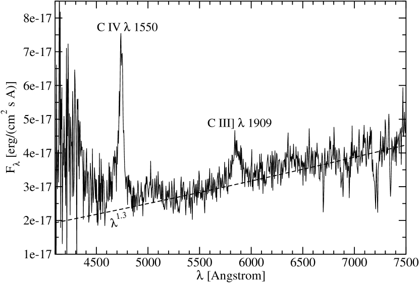
Figure 1: Optical spectrum of PKS 0528+134 on December 19, 2009, taken at the Steward Observatory. The two prominent emission lines of CIII] and CIV are labeled and correspond to luminosities of $L_{CIII]}\approx 4.2\times 10^{44}$ erg s^-1 and $L_{CIV}\approx 3.2\times 10^{45}$ erg s^-1. The continuum red-ward of $\sim 5000$ Å can be fit with a power-law $F_{\lambda}\propto\lambda^{1.3}$.

3.1.2 Optical Spectroscopy

In addition to the photometric observations described in the previous sub-section, PKS 0528+134 is also regularly monitored with spectroscopic observations through the University of Arizona – Steward Observatory Fermi Support program. As a representative example, we show in Figure 1, the optical spectrum of October 19, 2009, which is within the extended period of our multiwavelength campaign. The source was clearly still in the quiescent state targeted in this work.

The spectrum exhibits two distinct emission lines: CIII] $\lambda$1909, red-shifted to $\lambda=5860$ Å, and CIV $\lambda$1550, red-shifted to $\lambda=4740$ Å. The total measured flux in the lines corresponds to $F_{CIII]}=1.8\times 10^{-15}$ erg cm^-2 s^-1 and $F_{CIV}=4.3\times 10^{-15}$ erg cm^-2 s^-1. In order to evaluate the de-absorbed fluxes, we evaluate the extinction coefficients $A_{\lambda}$ with the extinction law of Cardelli et al. (1989) and $A_{V}=2.78$, yielding $A_{4740}=3.35$ and $A_{5860}=2.59$. This yields intrinsic luminosities in the two lines of $L_{CIII]}\approx 5.8\times 10^{44}$ erg s^-1 and $L_{CIV}\approx 2.5\times 10^{45}$ erg s^-1.

The continuum redward of $\sim 5000$ Å can be well fit with a power-law $F_{\lambda}\propto\lambda^{1.3}$, which corresponds to a steep spectrum in frequency space, $F_{\nu}\propto\nu^{-3.3}$.

Optical Polarimetry

R-band photo-polarimetric observations of PKS 0528+134 were also acquired with the 2.2 m telescope of the Calar Alto Observatory in Amería, Spain, as part of the MAPCAT program. The data were reduced and calibrated as described in Agudo et al. (2011) and Jorstad et al. (2010).

St. Petersburg observations were performed at the 70-cm telescope of Crimean Observatory using ST-7 XME photometer-polarimeter. The standard procedure, including bias and dark subtraction, flat-field correction and calibration relative to comparison stars 1, 2 and 3 from Raiteri et al. (1998) was applied.

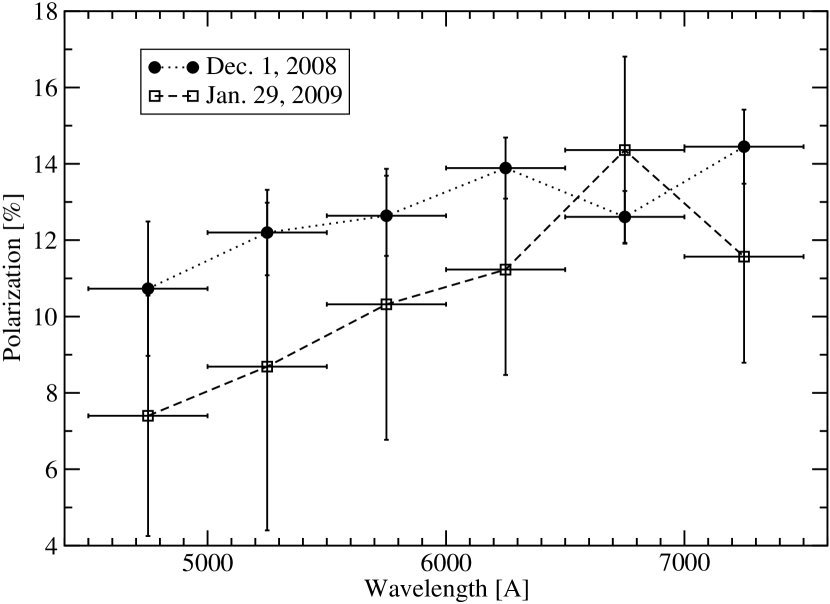
Figure 2: Wavelength dependence of the degree of polarization of the optical emission of PKS 0528+134, from two observations in 2008 December and 2009 January. The plot is highly suggestive of a systematic trend of increasing polarization with increasing wavelength.

Additional polarimetry and spectropolarimetry data were included from the University of Arizona – Steward Observatory Fermi Support program. Those data included two spectropolarimetric observations of PKS 0528+134 in 2008 December and 2009 January, which showed a rather high ($P\gtrsim 10$ %) degree of polarization, allowing for a meaningful spectrapolarimetric analysis. At those times, the object was in a similar quiescent state as during our campaign. The contributions of the CIII] and CIV lines (see previous sub-section) were assumed to be unpolarized, and their fluxes subtracted from the respective energy bins. Figure 2 shows the degree of polarization as a function of wavelength. The plot is highly suggestive of a systematic increase of the polarization towards longer frequencies. This may be interpreted as an increasing contribution of synchrotron emission towards the red end of the optical spectrum.

3.2 X-Ray Observations

3.2.1 XMM-Newton

PKS 0528+134 was observed by the XMM-Newton Observatory (Jansen et al., 2001) between September 8th and 14th 2009 on four consecutive revolutions. Table 1 summarizes these observations. Here, we focus on the data taken with the EPIC detector, covering the energy band between 0.2 and 10 keV. EPIC observations were taken in full frame mode and thin optical filter (except the pn exposure in 0600121501 that was taken on small window mode). XMM-Newton also has an Optical/UV Monitor Telescope (OM) (Mason et al., 2001), a small 30 cm telescope co-aligned with the main XMM-Newton X-ray telescopes. However, due to the optical faintness of PKS 0528+134 ($\gtrsim 19^{\rm th}$ mag), OM observations did not return useful data.

Obs. ID	Date	Exp. (pn)	CR (pn)	Exp. (MOS1)	CR (MOS1)	Exp. (MOS2)	CR (MOS2)
	yy/mm/dd	(ksec)	(cts/sec)	(ksec)	(cts/sec)	(ksec)	(cts/sec)
0600121401	2009-09-08$@$05:55UT	9.94(14.28)	0.2675$\pm$0.0052	15.2(22.1)	0.0897$\pm$0.0024	15.17(21.49)	0.0943$\pm$0.0025
0600121501	2009-09-10$@$06:05UT	19.89(20.13)	0.2194$\pm$0.0033	23.63(28.46)	0.0848$\pm$0.0019	24.38(28.48)	0.0897$\pm$0.0019
0600121601	2009-09-12$@$03:01UT	21.11(21.96)	0.2616$\pm$0.0035	26.5(26.5)	0.0808$\pm$0.0017	26.6(26.6)	0.0908$\pm$0.0018
0600121701	2009-09-14$@$02:52UT	$---$	$---$	26.68(35.61)	0.0754$\pm$0.0017	29.72(36.12)	0.0877$\pm$0.0017

Table 1: Summary of PKS 0528+134 XMM-Newton EPIC observations. Exp. = Livetime after (before) correction due to periods of higher background activity. CR = Count rates, given for the 0.2-10 keV energy range. The quadrant of the pn chip containing the source of the pn exposure in observation 0600121701 was lost and hence there is no source information.

Data Reduction

The data have been analysed using SASv9.0 (Gabriel et al., 2004) and corresponding calibration files. Event and source lists were obtained for the EPIC detector, following the standard SAS data reduction procedures. Several filtering criteria have been applied. The event list has been filtered for time periods of high background activity following the standard procedure of removing those time periods with background event rates at energies $E>10$ keV higher than 1.0 cts/sec and 0.8 cts/sec for EPIC-pn and EPIC-MOS, respectively. The time losses due to the removal of these periods are up to 30 % depending on the observation and the instrument (three out of the four observations were performed at the end of their respective revolutions with the consequent increase in radiation levels towards the end of the observations). Table 1 shows the livetimes for each observation and instrument before and after this correction has been performed. The data was also filtered to include only single and double (PATTERN$\leq$4) pattern events for EPIC-pn and single to quadruple (PATTERN$\leq$12) for EPIC-MOS as well as those with quality FLAG=0. The filtered event lists were used to generate light curves and spectral products. The source region was considered to be a circular region centered around the source. Annular background regions were chosen to be centered around the source with radii 60” $\leq$ R $\leq$ 80”. The source extraction regions were then optimized based on S/N for the given background region, which yielded typical values of $\sim$ 40” in radius for the source region.

	EPIC Power Law
	PHABS+PHABS
Obs ID	NH,mol	$\Gamma_{\rm ph}$	F0.2-2keV	F2-10keV	$\chi^{2}/d.o.f.$
	1022 cm-2		10-12 ergs cm-2 s-1	10-12 ergs cm-2 s-1
0600121401	0.15${}^{+0.04}_{-0.04}$	1.57${}^{+0.07}_{-0.07}$	0.28${}^{+0.03}_{-0.04}$ (0.88)	1.35${}^{+0.11}_{-0.11}$ (1.39)	0.93 (146.2/157)
0600121501	0.13${}^{+0.02}_{-0.03}$	1.60${}^{+0.05}_{-0.07}$	0.24${}^{+0.02}_{-0.03}$ (0.76)	1.10${}^{+0.07}_{-0.09}$ (1.14)	1.02 (243.3/238)
0600121601	0.17${}^{+0.02}_{-0.02}$	1.61${}^{+0.05}_{-0.02}$	0.24${}^{+0.02}_{-0.02}$ (0.81)	1.14${}^{+0.07}_{-0.06}$ (1.18)	1.05 (275.2/261)
0600121701	0.12${}^{+0.64}_{-0.56}$	1.58${}^{+0.07}_{-0.10}$	0.26${}^{+0.03}_{-0.02}$ (0.69)	1.18${}^{+0.11}_{-0.11}$ (1.22)	0.99 (135.6/137)

Table 2: Fit performed in the 0.2 – 10 keV energy range. All 3 EPIC instruments have been used simultaneously in the fit. The Galactic absorption traced by 21-cm emission from neutral hydrogen, N_H,21cm has been fixed to a value of $0.24\cdot 10^{22}$ cm^-2 according to the LAB Survey of Galactic HI Kalberla et al. (2005). Fluxes given are not absorption corrected (in parenthesis the de-absorbed flux is given). Errors indicate the 90 % CL. NOTE: For observation id 0600121701 only MOS1 and MOS2 are available. In this case, the fit has been performed in the 0.3 – 10 keV energy range and the fluxes given are between 0.3 – 2.0 and 2.0 – 10 keV.

EPIC Spectral Analysis

Time-averaged spectra have been obtained for each individual observation. The spectra were re-binned in order not to oversample the intrinsic energy resolution of the EPIC cameras by a factor larger than 3, while making sure that each spectral channel contains at least 25 background-subtracted counts. Both conditions allow the use of the $\chi^{2}$ quality-of-fit estimator to find the best fit model. Fits were performed in the 0.2 – 10 keV energy range. The spectra from all three EPIC cameras have been used simultaneously during the fitting procedure. The systematic difference between the EPIC cameras is below $\sim 5$ % in normalization. For the spectral analysis and fitting procedure, XSPEC v12.4 (Arnaud, 1996) was used.

The spectral model used to fit the data is composed of a power law convolved with a combination of Galactic column density of absorbing material traced by 21-cm emission from atomic hydrogen (N_H,21cm), plus an additional absorbing column density (N_H,mol), primarily due to heavy elements in the intervening molecular cloud B30, which are not properly traced by the hydrogen column density. The Galactic hydrogen column density is kept fixed during the fitting procedure. The spectral fitting model takes the following form for the differential photon flux $\Phi(E)$:

$$\Phi(E)=e^{-N_{\rm H,21cm}\sigma(E)}\cdot e^{-N_{\rm H,mol}\sigma(E)}\cdot N\cdot E^{-\Gamma_{\rm ph}}$$ (1)

where $\sigma(E)$ is the photoelectric absorption cross-section, with abundances after Anders & Grevesse (1989), and $\Gamma_{\rm ph}$ the power-law index with normalization N. Errors in the relevant parameters are given at the 90 % confidence level (CL) for any given parameter.

Table 2 shows the best fit values for the model considered for all four observations. Figure 3 shows an example of the spectra as determined for one of the observations (composed of EPIC-pn and the two EPIC-MOS spectra) with the best fit model and $\chi^{2}$ deviation. Similar spectra are derived for the other observations.

Figure 3: Example of EPIC (pn, MOS1 and MOS2) spectrum for the observation id 0600121601 where EPIC data is available for all three cameras. The fit has been done in the 0.2-10 keV energy range with channel grouping $>3$ channels and $>25$ background subtracted counts.

3.2.2 RXTE

In addition to our four ToO XMM-Newton pointings, we monitored the 2.4 – 10 keV X-ray flux of PKS 0528+134 with the Rossi X-ray Timing Explorer (RXTE) Proportional Counter Array (PCA), with exposure times of 900 – 3400 s for individual observations. The X-ray flux measurement entailed the subtraction of an X-ray background model (faint source model, version 20051128) from the raw spectrum using the standard X-ray data analysis software packages FTOOLS and XANADU. We used the program XSPEC to fit the residual photon spectrum with a power-law model plus photoelectric absorption along the line of sight.

3.2.3 Suzaku

PKS 0528+134 was also observed with the Suzaku satellite as a part of multi-band observations conducted in September 2008, about one year prior to the campaign covered in this paper. However, both the X-ray flux and $\gamma$-ray flux levels were comparable to those measured during the September 2009 campaign, indicating a quiescent state. We therefore include the Suzaku data here for comparison of the spectral and short-term variability properties with those measured by XMM-Newton one year later, in a similar quiescent state. The Suzaku satellite features instruments sensitive in the soft X-ray band.

Suzaku observations of PKS 0528+134 started on 2008 September 27, 02:38 UT, and lasted until 2008 October 2, 16:12 UT. Since the source was not detected in the Hard X-Ray Detector (HXD) data, we considered only the X-Ray Imaging Spectrometer (XIS) instruments. The observation conditions were nominal, although the XIS1 data suffered from unusually high and variable background, resulting in a total apparent background count rate ranging from 1 to 3 counts s^-1 over the entire chip. Nonetheless, since the background-subtracted spectrum determined from the XIS1 data was entirely consistent with that from XIS0 and XIS3, we included the properly background-subtracted XIS1 data in the spectral fitting (see below).

Figure 4: Suzaku X-ray light curve of PKS 0528+134 from the XIS3 data of 2008 September 27 – October 2. $t=0$ corresponds to MJD 54736.1771.

The total exposure time yielding good data accumulated in the pointing was 203 ks. We used the standard ftools data reduction package, provided by the Suzaku Science Operations Center, with the calibration files included in the CALDB ver. 4.3.1. The net count rates were, respectively, 0.10, 0.13, and 0.12 count s^-1 for XIS0, XIS1, and XIS3. For the analysis of spectra and light curves, we extracted the counts from a region corresponding to a circle with 260 arc sec radius. We used a region of a comparable size from the same chip to extract the background counts. We plot the resulting total light curve (not background-subtracted) from XIS3, binned in 5400 sec bins, in Figure 4, and note that the background was steady at the level of $\sim 0.015$ count s^-1. The data indicate no significant rapid (a day or less) variability during the Suzaku observation, but show a long-term trend, with a $\sim 20$ % decrease in flux over the $\sim 5.3$ day long duration of the observation. A similar secular flux decrease is seen in the two other XIS detectors.

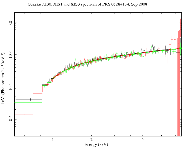
Figure 5: 0.5 – 10 keV X-ray spectrum of PKS 0528+134 from the Suzaku observations of 2008 September 27 – October 2.

For the spectral analysis, we we used the XSPEC spectral analysis software (Arnaud, 1996). For the spectral fitting, we used the standard redistribution files and mirror effective areas generated with Suzaku-specific tools. We included the counts corresponding to the energy range of 0.5 – 10.0 keV in our spectral fits. We used all three XIS detectors simultaneously, but allowed for a small (a few %) variation of the relative normalizations. The source spectrum was modeled as an absorbed power law, with the cross-sections and elemental abundances as given in Morrison & McCammon (1983). Other absorption models give similar results. The best-fit absorbing column was $4.6\pm 0.2\times 10^{21}$ cm^-2, and the photon index was $1.54\pm 0.03$, with the acceptable best-fit $\chi^{2}$ of 3407 for 3512 d.o.f. The Suzaku spectrum is shown in Figure 5. The observed model 2 – 10 keV flux is $2.8\times 10^{-12}$ erg cm^-2 s^-1, with the statistical error of 5 %, which is probably smaller than the systematic error resulting from the calibration uncertainty of the Suzaku instruments.

The fitted values of the total absorbing column are only marginally consistent between the Suzaku and XMM-Newton data sets. This might be in part related to the differences in calibration of the two instruments. An additional source for the discrepancy might be the fact that (1) we are using Galactic elemental abundances, which might or might not be appropriate for the line-of-sight molecular cloud, and (2) the bandpass of XMM-Newton extends down to 0.3 keV, while for Suzaku it is 0.5 keV. If the elemental abundances in the intervening absorber of low-z elements are not the same in the molecular cloud as the Galactic abundances assumed in the spectral fit, the precise value of the best-fit $N_{H}$ might be dependent on the bandpass of the instrument and even the details of the effective area at the energies where the absorption edges due to those elements play an important role.

While the X-ray spectral index measured by Suzaku in 2008 September/October is consistent with the value measured one year later by XMM-Newton (see §3.2.1, table 2), the Suzaku 2 – 10 keV flux is about a factor 2.4 higher than the XMM-Newton value. This is in agreement with the $\sim$ factor 2 – 3 variability measured by RXTE on $\sim$ weekly time scales (see §4.1).

3.3 $\gamma$-Ray Observations

Gamma-ray observations of PKS 0528+134 were performed by the Fermi-LAT. This is a pair-conversion $\gamma$-ray telescope sensitive to photon energies greater than 20 MeV. In its nominal scanning mode, it surveys the whole sky every 3 hours with a field of view of about 2.4 sr (Atwood et al., 2009). The data presented in this paper (restricted to the 100 MeV – 200 GeV range) were collected from MJD 54983 (2009 June 1st) to MJD 55193 (2009 December 28). For this analysis, the Diffuse event class was used. This is the optimized class for point source analysis with minimal residual contamination from charged-particle backgrounds. To minimize systematics, only photons with energies greater than 100 MeV were considered in this analysis. In order to limit the contamination from atmospheric $\gamma$-rays produced by interactions of cosmic rays with the upper atmosphere of the Earth, only events with zenith angle $<$ 105^∘ were selected. In addition, time intervals during which the rocking angle was larger than 52^∘ have been excluded from the analysis, because the bright limb of the Earth enters the field of view. The analysis was performed with the standard analysis tool gtlike, part of the Fermi-LAT Science Tools software package (version v9r15p5). The P6_V3_DIFFUSE set of instrument response functions was applied.

Photons were selected in a circular Region Of Interest (ROI) 7^∘ in radius, centered at the position of PKS 0528+134. The isotropic background, including the sum of residual instrumental background and extragalactic diffuse $\gamma$-ray background, was modeled by fitting this component at high galactic latitude (file provided with Science Tools). The Galactic and Isotropic diffuse emission models version “gll_iem_v02.fit” and “isotropic_iem_v02.txt” were used. All point sources in the first Fermi-LAT catalog (Abdo et al., 2010c) lying within the ROI and a surrounding 10^∘-wide annulus were considered in the fit and modeled with single power-law distributions of the form $F(E)=N_{0}(E/E_{0})^{-\Gamma}$. Their flux was kept free whereas their spectral index value was frozen to the value listed in the 1FGL catalog, except for PKS 0528+134 whose index was kept free. Due to limited statistics, the gamma-ray spectrum of PKS 0528+134 was modeled with a power-law distribution in the present analysis, although the spectrum measured over 11 months covered by the 1FGL catalog exhibits distinct curvature, characterized by a curvature index of 8.14, corresponding to a 4 % probability that the spectrum is adequately represented by a power law (Abdo et al., 2010a). The highest energy photon attributed to PKS 0528+134 has an energy of 8.6 GeV. The estimated systematic uncertainty on the flux is 10 % at 100 MeV, 5 % at 500 MeV and 20 % at 10 GeV.

3.4 Radio Observations

We obtained radio observations from the GLAST-AGILE Support Program (GASP) of the Whole Earth Blazar Telescope (WEBT). In table 3, we list the frequencies in which we collected data and the observatories participating in the campaign.

Table 3: Frequencies and observatories used to collect radio data

Frequency	Observatory
05 GHz	UMRAO, MEDICINA
08 GHz	UMRAO, MEDICINA
14 GHz	UMRAO
22 GHz	MEDICINA
37 GHz	Mets hovi Radio Observatory (KURP-GIX)
43 GHz	Noto
230 GHz	MAUNA KEA (SMA)
345 GHz	MAUNA KEA (SMA)

Centimeter-band observations were obtained with the University of Michigan 26-meter prime focus paraboloid equipped with radiometers operating at central frequencies of 4.8, 8.0, and 14.5 GHz. Observations at all three frequencies utilized rotating polarimeter systems permitting both total flux density and linear polarization to be measured. A typical measurement consisted of 8 to 16 individual pointings over a 20 – 40 minute time period. Frequent drift scans were made across stronger sources to verify the telescope pointing correction curves. Observations of program sources were intermixed with observations of a grid of calibrator sources to correct for temporal changes in the antenna aperture efficiency. The flux scale was based on observations of Cassiopeia A (see, e,g., Baars et al., 1977). Details of the calibration and analysis techniques are described in Aller et al. (1985).

The 37 GHz observations were made with the 13.7 m diameter Metsähovi radio telescope. The detection limit of the telescope at 37 GHz is of the order of 0.2 Jy under optimal conditions. Data points with a SNR $<4$ are handled as non-detections. The flux density scale is set by observations of DR 21. Sources NGC 7027, 3C 274 and 3C 84 are used as secondary calibrators. A detailed description of the data reduction and analysis is given in Teräsranta et al. (1998). The error estimate in the flux density includes the contribution from the measurement rms and the uncertainty of the absolute calibration.

The 43 GHz Noto observations have been performed using the On The Fly (OTF) scan technique (scan duration about 20 s) and the telescope gain (K/Jy) was determined as a function of the elevation using NGC 7027 as primary calibrator. To improve the signal to noise ratio many scans have been acquired and then averaged for a total integration time of about 15 minutes. The antenna temperature has been estimated by a gaussian fit of the average scan. A more detailed description for the 43 GHz data is given by Leto et al. (2009). Radio observations at the Medicina radio observatory were performed at 5, 8, and 22 GHz, and were analyzed as detailed in Bach et al. (2007).

Data at 230 GHz and 345 GHz were collected at the Submillimeter Array (SMA) on Mauna Kea and reduced using the MIR data reduction software. SMA flux density measurements are produced from a mixture of dedicated flux calibration/monitoring observations and data from science projects that may utilize a quasar as a calibration standard (typically for gain calibration of the interferometer). Raw visibility data are calibrated to correct for atmospheric absorption and instrumental gain variations, and then referenced to observations of standard flux calibration sources, generally planets and/or moons. More details on the SMA flux density monitoring program can be found in Gurwell et al. (2007).

4 Variability Analysis

One of the main goals of this multiwavelength campaign was the search for flux and spectral variability of PKS 0528+134 in its quiescent state. We first describe our results on flux variability in §4.1 and then turn to the investigation of spectral variability in §4.2. In §4.3 we discuss variability of the optical polarization.

4.1 Flux Variability

The optical light curves of PKS 0528+134 obtained with the 1.3-m McGraw-Hill telescope of the MDM Observatory during the core of our multiwavelength campaign (September 9 – September 19, 2009), along with the publically available SMARTS data from the same period, are plotted in figure 6. An increase in the brightness of the source of $\sim$ 0.7 magnitudes in the R and V filters around JD 2455086 (September 11) is evident. In order to quantify the variability, we computed the reduced $\chi^{2}$ for a fit to a constant flux. Variability is evident in all three bands with $\chi_{\nu}^{2}=15.9$, $5.2$, and $26.2$, respectively, for the R, V, and B bands. Due to the limited observability period of PKS 0528+134 in any given night (typically $\lesssim 4$ hr), the light curve during this mini-flare is clearly undersampled. Due to the sparse sampling of the optical observations, we can only constrain the variability time scale to $t_{\rm var}^{\rm opt}\lesssim 1$ day.

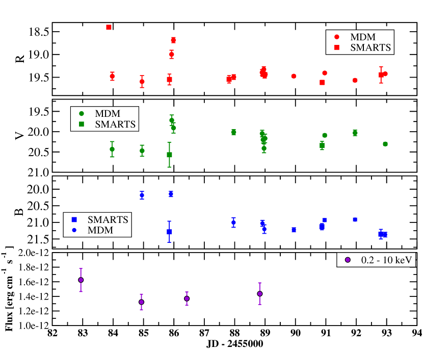
Figure 6: MDM and SMARTS optical light curves (RVB) of PKS 0528+134 between September 9 and 19, 2009. The bottom panel shows the X-ray light curve corresponding to the four XMM-Newton observations.

In the same way, we analyzed the X-ray variability on time scales of $\sim 1$ – 2 day between our four XMM-Newton observations as well on time scales of a few hours, within the individual observations. The XMM-Newton light curve is plotted in the bottom panel of figure 6. No flux variability is evident. For the 0.2 – 10 keV X-ray flux, a fit to a constant results in a $\chi_{\nu}^{2}$ of 0.91, thus confirming the absence of significant variability. For the same XMM-Newton observations, we also analyze the intraday variability. For most observations the $\chi_{\nu}^{2}$ for a fit to a constant flux is less than 1. In figure 7, we show the light curve from the XMM-Newton MOS1 data of September 10, 2009, as an example. For this particular observation, $\chi_{\nu}^{2}\approx 0.81$ is found.

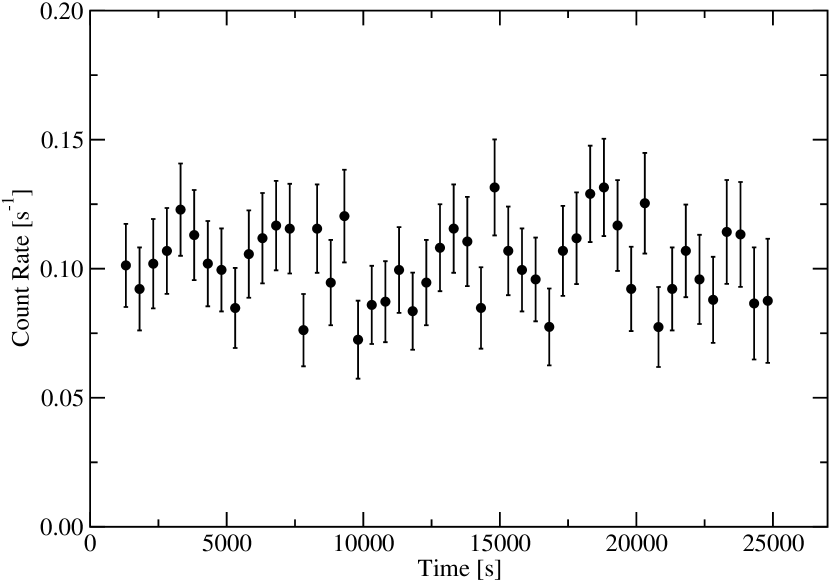
Figure 7: XMM-Newton MOS1 light curve of our ToO observation on September 10, 2009. Each point corresponds to a bin of 500 seconds. No evidence for intra-day variability is found.

A multiwavelength variability analysis for a more extended period of time was made possible by including RXTE monitoring data. In figure 8, we show the light curves of PKS 0528+134 in radio (5 and 37 GHz), optical, X-rays (RXTE), and $\gamma$-rays (bottom to top). The vertical shaded band highlights the interval of the core campaign where the most intense optical and X-ray observations (including XMM-Newton) were performed. The RXTE X-ray data from the period July 14 to December 2, 2009, represent the most extended coverage. In this interval, PKS 0528+134 shows significant variability corresponding to a reduced $\chi_{\nu}^{2}$ of 3.83 for a fit to a constant flux. The RXTE light curve indicates variability with flux changes of $|\Delta F/F|\sim 50$ % on a characteristic time scale of $t_{\rm var}^{X}\sim 1$ week.

We note here that the fluxes resulting from our RXTE analysis are systematically higher than those measured by XMM-Newton during the same period. We have carefully double- and cross-checked both analyses and confirmed this discrepancy. The ROSAT All Sky Survey Catalogue does not list any known source in the field of view of RXTE which may be responsible for the flux discrepancy. Furthermore, three RXTE observations were carried out within a few hours of one of the XMM-Newton observations. Given this short time period and the systematic offset between the two instruments, rapid variability appears unlikely to cause the flux discrepancy. The factor of 4 discrepancy seems also too large to be solely due to calibration uncertainties. A plausible explanation for the systematic offset could lie in an uncertain background model for the RXTE analysis in the region around PKS 0528+134, near the Galactic anti-center. While this would cause a constant offset of the RXTE flux levels, it will not affect the variability. We are therefore confident that the RXTE flux variability analysis presented here is robust. For the analysis of the spectral energy distributions in §6, the flux and spectral information from XMM-Newton will be used.

The optical light curve (second panel from the bottom of Figure 8), including data from the MDM, SMARTS, Perkins, San Pedro Mártir, Calar Alto, and Crimean observatories, covers the interval from September 9 to November 19, 2009. This is the band where PKS 0528+134 shows the most significant variations in its flux density, with flaring episodes exhibiting brightness changes of $\Delta R\lesssim 1^{\rm mag}$ on a time scale of $\lesssim 1$ day.

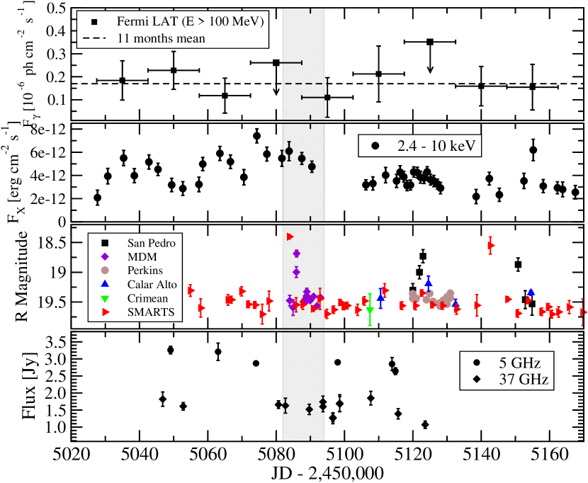
Figure 8: Light curves of PKS 0528+134. From top to bottom: a) the Fermi $\gamma$-ray flux in 15-day integration bins. b) X-ray (RXTE) light curve. c) Optical (R-magnitude) light curve including data from the MDM, SMARTS, Perkins, San Pedro Mártir, Calar Alto, and Crimean observatories. d) Radio light curves at 5 and 37 GHz.

As shown in figure 8 (top panel), the Fermi $\gamma$-ray flux does not present significant variability during the extended campaign period (2009 July – December). The best fit found for the flux (E $>$ 100 MeV) is $(0.12\pm 0.02)\times 10^{-6}$ ph cm^-2 s^-1 with a test statistic TS = 68. The Test Statistic (Mattox et al., 1996) is defined as twice the difference in log(likelihood) obtained by including the source of interest and omitting it in the source model used in the gtlike analysis. This flux is slightly lower than the mean flux observed over the first eleven months of Fermi data (Abdo et al., 2010a), which corresponds to $(0.17\pm 0.01)\times 10^{-6}$ ph cm^-2 s^-1 as represented by the dashed horizontal line in the same panel.

Among the frequencies monitored in the radio regime, the 5 GHz and 37 GHz light curves had the most extended coverage in time. In the bottom panel of figure 8, we show both light curves. Only moderate variability with amplitudes of $|\Delta F/F|\lesssim 20$ % is observed at these frequencies. In particular, a decreasing flux tendency is found at the end of the 37 GHz light curve. A fit to a constant flux results in $\chi_{\nu}^{2}=3.92$ and 2.61 for the 5 GHz and 37 GHz light curves, respectively.

A more detailed analysis of the radio regime, including the light curves in all the monitored radio frequencies, is presented in figure 9. The radio light curves show moderate variability in general. The 8 GHz and 14 GHz bands present significant flux variations with $\chi_{\nu}^{2}=32.96$ and 10.17, respectively, for a fit to a constant flux. The results of a similar analysis for all radio frequencies are summarized in Table 4. Variability appears to occur on time scales of $t_{\rm var}^{\rm radio}\sim 1$ – 2 weeks, comparable to the X-ray variability time scale measured by RXTE (see above).

Table 4: Light curve variability analysis in radio frequencies: $\chi_{\nu}^{2}$ for fits to a constant flux.

Frequency	$\chi_{\nu}^{2}$
5 GHz	3.92
8 GHz	32.96
14 GHz	10.17
37 GHz	2.61
230 GHz	0.62

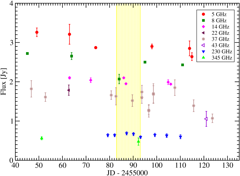
Figure 9: Radio light curves of PKS 0528+134. The vertical yellow shaded band corresponds to the interval when MDM optical and XMM-Newton X-ray observations of this source were performed.

In summary, the comparative flux variability analysis of PKS 0528+134 at different frequencies from $\gamma$-rays through radio indicates no significant variability in the $\gamma$-ray regime, moderate variability in the X-rays ($|\Delta F/F|\sim 50$ %) and most radio frequencies ($|\Delta F/F|\lesssim 20$ %) on time scales of $\sim 1$ – 2 weeks, and variability of up to $\Delta R\lesssim 1^{\rm mag}$ in the optical bands on time scales of several hours. Our data are not sampled densely enough for a meaningful analysis of time lags among different bands.

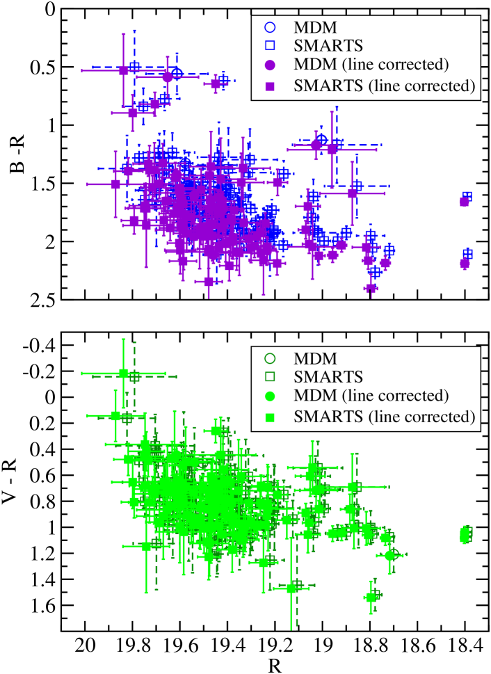
Figure 10: Color-magnitude diagrams for B - R (top panel) and V - R (bottom panel) vs. R-band magnitude. Open symbols with dashed error bars indicate the original data; filled symbols with solid error bars show the data data after correction of all magnitudes for the contributions from the CIII] and CIV emission lines.

4.2 Spectral Variability Analysis

In order to test whether the optical flux variability discussed in the previous section is associated with spectral changes, we evaluated color indices B - R and V - R as a measure of spectral hardness. These were calculated for any pair of B (V) and R magnitudes measured quasi-simultaneously, i.e., during the same night, by MDM and SMARTS. If conditions were good enough to extract more than one high-quality (error in magnitude $<0.1$) V or B and R band data point per night, magnitude measurements taken within $<1$ hr of each other were used to calculate color indices. The resulting flux – spectral hardness correlations, indicated by the color-magnitude diagrams (color vs. R magnitude), are shown by the open symbols with dashed error bars in Figure 10. The data clearly indicate color variability. Specifically, a weak softer-when-brighter trend seems to be present in both diagrams.

A correlation analysis of the color-magnitude data sets yields a Pearson’s correlation coefficient of $r=-0.50$, for the V - R color vs. R magnitude correlation, and $r=-0.45$ for the B - R color. In both cases the obtained correlation coefficients indicate a weak negative correlation between color and magnitude, which confirm the redder-when-brighter trend. In order to assess the significance of these color correlations, we performed Monte-Carlo simulations of 10 million data sets with the same number of data points and the same spread in values as our data. The R magnitudes and color indices are assumed to be randomly distributed and not correlated to each other. For each simulated data set, the Pearson’s correlation coefficient was evaluated in the same way as done for our observational data. This resulted in a chance probabilities of $P(<r)=5\times 10^{-6}$ and $P(<r)=2\times 10^{-7}$, respectively, of obtaining a correlation coefficient more negative than the ones resulting from our observational data. This seems to provide strong evidence for the presence of a redder-when-brighter trend in PKS 0528+134.

Such a redder-when-brighter trend has been observed in other FSRQs, e.g., 3C 454.3 (Raiteri et al., 2008), where it has been partially attributed to a contribution of emission lines from the BLR to the B band. In order to test whether this may also be the cause of the color variability described above, we utilize the line fluxes inferred from the spectrum shown in Figure 1. We note that the red-shifted CIV line falls within the B-band range. At $\lambda=4740$ Å, the B-band filter has a transmission coefficient of approximately $f_{\lambda}=70$ % of its maximum value. Hence, using the bandwidth of the B filter of $\Delta\nu=1.4\times 10^{14}$ Hz, we find that the CIV line will make an effective contribution of $F_{\nu,CIV}^{B}=F_{CIV}\,f_{\lambda}/\Delta\nu\approx 2.1\,\mu$ Jy to the B-band flux. An analogous calculation of the contribution from the CIII] line to the V and R bands yields $F_{\nu,CIII]}^{V}\approx 1.0\,\mu$Jy and $F_{\nu,CIII]}^{R}\approx 1.6\,\mu$Jy. We corrected all B, V, and R magnitude values for these line contributions and re-evaluated the color magnitude correlations. The resulting points are shown as solid symbols in Figure 10. This leads to an overall slight shift towards fainter (larger R) magnitudes and redder B - R colors. However, the overall color variability trend and its significance remain unaffected by this correction.

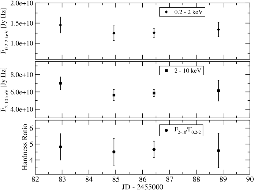
Figure 11: Light curves in soft (0.2 – 2 keV) X-rays (top panel), hard (2 – 10 keV) X-rays (middle), and the hardness ratio. No significant spectral variability was found.

We also analyzed the spectral variability in the X-ray regime. For the XMM-Newton data, we analyzed the variability of the hardness ratio $F_{2-10keV}/F_{0.2-2keV}$. Figure 11 illustrates that the hardness ratio is consistent with being constant over the four XMM-Newton observations performed as part of the core campaign. The RXTE X-ray energy index $\alpha$ was analyzed over a period of 150 days as plotted in the top panel of figure 12. A fit to a constant results in $\chi_{\nu}^{2}=1.31$ is found, indicating very moderate spectral variability. The comparison of the XMM-Newton spectra with the Suzaku spectrum from 2008 September/October (see §3.2.3) suggests that the X-ray spectral index remains stable on very long time scales, even throughout substantial (factor $\sim 2$ – 3) flux variations.

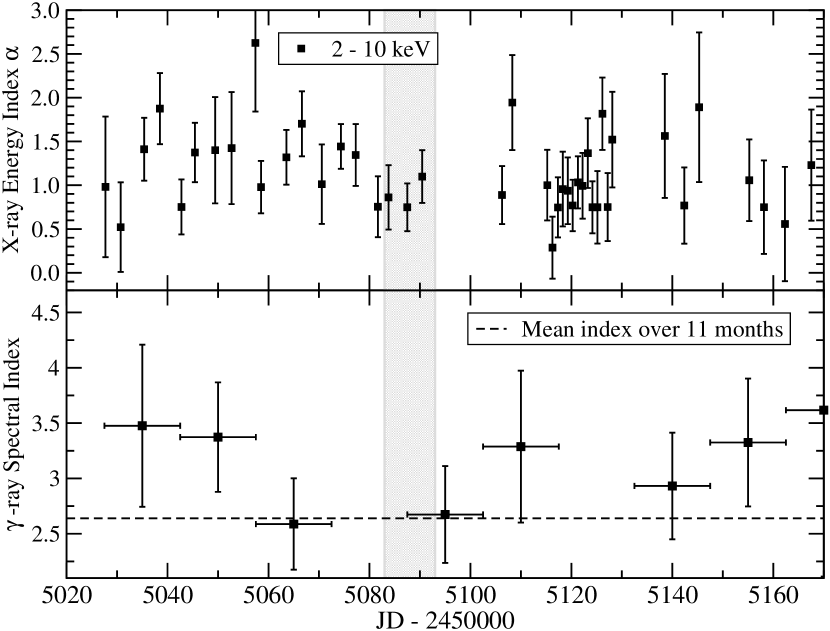
Figure 12: Top panel: X-ray (2 – 10 keV) energy spectral index $\alpha$ vs. time. Bottom: Fermi $\gamma$-ray photon spectral index ($\Gamma_{\rm ph}=\alpha+1)$ vs. time. The dashed horizontal line corresponds to an index of 2.64, the mean index observed over the first eleven months of Fermi data.

We also analyzed the Fermi $\gamma$-ray spectral index variability over the extended campaign period. As shown in the bottom panel of figure 12, no significant variability is found. The best fit found for the spectral index in this period of time is $\Gamma=2.9\pm 0.2$, which is slightly softer than the mean spectral index ($\Gamma=2.64\pm 0.06$) observed over the first eleven months of Fermi data (dashed horizontal line Abdo et al., 2010a).

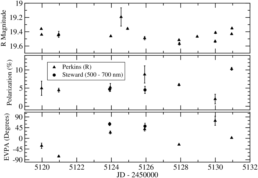
Figure 13: Simultaneous photometric and polarimetric data for PKS 0528+134 on seven days during October 15 – 26, 2009. Top panel: R-band magnitude. Middle panel: Degree of polarization. Bottom panel: Electric vector position angle (EVPA). While there is significant variability in the R-band flux, degree of polarization, and EVPA, we did not find a significant correlation between polarization and flux states.

4.3 Optical Polarization Variability Analysis

The polarization variability analysis on PKS 0528+134 was performed using the R-band polarimetric observations at the 1.8 m Perkins telescope of Lowell observatory during a twelve day period from October 15 to 26, 2009, and two measurements from the University of Arizona / Steward Observatory Fermi support program from the same period. As shown in figure 13, the Perkins polarimetry data indicate strong variability of the degree of polarization ($\chi_{\nu}^{2}=20.2$ for a fit to a constant) and the electric vector position angle (EVPA). The variability of the polarization parameters occurs on time scales of $\sim 1$ – 2 days and shows no obvious correlation with the fluxes in the optical or any other wavelength band.

The significant degree of polarization in the optical (and radio) hints towards a substantial synchrotron contribution to the emission at these wavelengths. We will discuss implications of our polarization results in Section 7.

5 Structure of the Parsec Scale Jet

The quasar PKS 0528+134 is monitored monthly by the Boston University (BU) group with the Very Long Baseline Array (VLBA) at 43 GHz within a sample of bright $\gamma$-ray blazars . The source was also included in a 2-week campaign of observations of 12 $\gamma$-ray blazars organized in 2009 October when 3 additional VLBA epochs at 43 GHz were obtained (VLBA project S2053). Figure 14 shows the total and polarized intensity images of the quasar in 2009 Autumn. The VLBA data were calibrated, imaged, and modeled in the same manner as discussed in Jorstad et al. (2005). As we did for the optical data, the polarization parameters were evaluated taking into account the statistical bias as detailed in Wardle & Kronberg (1974). Table 5 gives the parameters (flux, position, size, degree and position angle of polarization) of the main features seen in the radio jet during this period. Figure 15 shows the light curve of the VLBI core at 43 GHz of the quasar over the last three years as monitored by the BU group. According to Figure 15 the parsesc scale jet of PKS 0528+134 was in a quiescent state in 2009 Autumn. The core was moderately polarized, $P\sim 2$ %, with a stable position angle of polarization in a range between 42^∘ and 50^∘ that aligns within 10^∘ with the jet direction as determined by the position angle of the brightest knot $C2$ with respect to the core. The closest knot to the core, $C1$, has the highest level of polarization, $P\sim 10$ %, with the position of polarization perpendicular to the local jet direction. Although we do not observe superluminal knots in 2009 Autumn, the quasar is known to have a very high apparent speed in the jet, implying a high bulk Lorentz factor, $\Gamma\sim 30$ (Jorstad et al., 2005).

Table 5: Parameters of Jet Components

Epoch	Knot	S [Jy]	R [mas]	$\Theta$ [∘]	a [mas]	P [%]	$\chi$ [∘]
(1)	(2)	(3)	(4)	(5)	(6)	(7)	(8)
16 Sep	$A0$	0.842$\pm$0.085	0.0	$\cdots$	0.048	2.5$\pm$0.8	47$\pm$7
	$C1$	0.14$\pm$0.025	0.165$\pm$0.025	71.5$\pm$0.5	0.107	12.3$\pm$2.2	$-$12$\pm$8
	$C2$	0.35$\pm$0.050	0.70$\pm$0.05	64.3$\pm$0.5	0.522	$<$2.0	$\cdots$
14 Oct	$A0$	0.702$\pm$0.065	0.0	$\cdots$	0.000	1.4$\pm$0.6	49$\pm$8
	$C1$	0.14$\pm$0.025	0.136$\pm$0.025	82.4$\pm$0.5	0.187	8.0$\pm$2.5	0$\pm$10
	$C2$	0.29$\pm$0.050	0.71$\pm$0.05	61.8$\pm$1.0	0.568	5.4$\pm$1.8	93$\pm$5
16 Oct	$A0$	0.794$\pm$0.055	0.0	$\cdots$	0.035	1.0$\pm$0.5	50$\pm$8
	$C1$	0.25$\pm$0.025	0.127$\pm$0.025	68.7$\pm$0.5	0.250	8.2$\pm$2.0	$-$3$\pm$10
	$C2$	0.37$\pm$0.07	0.72$\pm$0.05	63.4$\pm$0.5	0.510	4.0$\pm$1.5	91$\pm$8
20 Oct	$A0$	0.826$\pm$0.065	0.0	$\cdots$	0.023	2.1$\pm$0.6	42$\pm$5
	$C1$	0.21$\pm$0.025	0.143$\pm$0.025	69.4$\pm$0.5	0.240	$<$5	$\cdots$
	$C2$	0.36$\pm$0.05	0.72$\pm$0.05	64.2$\pm$0.5	0.490	4.4$\pm$1.5	91$\pm$6
28 Nov	$A0$	0.794$\pm$0.045	0.0	$\cdots$	0.035	$<$1.0	$\cdots$
	$C1$	0.25$\pm$0.02	0.137$\pm$0.025	68.7$\pm$0.5	0.250	$<$4	$\cdots$
	$C2$	0.37$\pm$0.05	0.72$\pm$0.05	63.4$\pm$0.5	0.510	$<$2.4	$\cdots$

Note. — Columns: 1 - epoch of the observation; 2 - component designation; 3 - flux of component; 4 - distance of component from the VLBI core; 5 - position angle of component with respect to the core; 6 - diameter of component; 7 - degree of polarization of component; 8 - position angle of polarization of component

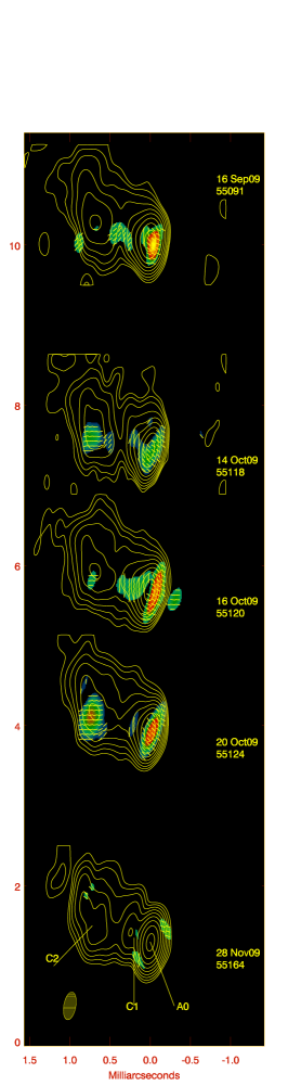
Figure 14: 43 GHz total (contours) and polarized (color scale) intensity images of PKS 0528+134 during 2009 Autumn. The highest contour corresponds to $S_{\rm peak}$=850 mJy/beam, while the yellow color indicates the highest polarized flux of $S_{\rm peak}^{\rm p}=30$ mJy/beam, for a beam of $0.33\times 0.15$ mas² at PA=-10^∘. Total intensity contours correspond to 0.25, 0.5, …, 64 % of the peak. Sticks over the polarized intensity contours indicate the plane of polarization. The designation of components corresponds to Table 5.

Figure 15: Light curve of the VLBI core at 43 GHz. The vertical lines indicate the period of intensified monitoring in 2009 Autumn.

6 Spectral Energy Distributions (SEDs) Modeling

In figure 16, we present the SEDs of PKS 0528+134 from radio to $\gamma$-rays (blue filled circles) corresponding to the four XMM-Newton observations (September 8, 10, 11, 14). The optical data have been dereddened assuming $A_{V}$=2.782, $A_{B}=3.62$ and $A_{R}=2.24$, as given in the NASA/IPAC Extragalactic Database according to the sky dust map given by Schlegel et al. (1998). We found in sections 4.1 and 4.2 that the Fermi $\gamma$-ray flux and spectral index of PKS 0528+134 did not show significant variability in the interval including the core campaign. Accordingly, the same $\gamma$-ray spectrum was used in the four SEDs. As in its flare states, in this quiescent state the SED of PKS 0528+134 is characterized by two peaks, a low-energy peak between the far infrared and optical spectral bands, and a high-energy peak at MeV – GeV energies. As can be seen, in all the SEDs the high-energy component dominates the bolometric output by a large amount.

We produce model fits to all four SEDs using the equilibrium version of the leptonic one-zone model developed by Böttcher & Chiang (2002). This equilibrium model is described in more detail in Acciari et al. (2009), and we here summarize its main features. The observed electromagnetic radiation is interpreted as originating from ultrarelativistic electrons (and positrons) in a spherical emission region of co-moving radius $R$, which is moving with a relativistic speed $\beta_{\Gamma}c$, corresponding to the bulk Lorentz factor $\Gamma$. Depending on the viewing angle $\theta$ between the jet direction and the line of sight, the transformations of photon energies and fluxes is characterized by the Doppler factor $D=\left(\Gamma[1-\beta_{\Gamma}\cos\theta]\right)^{-1}$. The size of the emission region is constrained by the shortest observed variability time scale $\delta t_{\rm var,min}$ through $R\leq c\delta t_{\rm var,min}\,D/(1+z)\lesssim 8\times 10^{15}(\delta t_{\rm var,min}/{\rm d})\,(D/10)$ cm.

Ultrarelativistic electrons are assumed to be instantaneously accelerated at a height $z_{0}$ above the accretion disk into a power-law distribution in electron energy, $E_{e}=\gamma m_{e}c^{2}$, at a rate per unit volume and unit Lorentz factor interval given by $Q(\gamma)=Q_{0}\gamma^{-q}$ with a low- and high-energy cutoffs $\gamma_{1}$ and $\gamma_{2}$, respectively, and injection spectral index $q$. An equilibrium between this particle injection, radiative cooling, and escape of particles from the emission region yields a temporary equilibrium state described by a broken power-law. The time scale for particle escape is parameterized through an escape time scale parameter $\eta_{\rm esc}>1$ as $t_{\rm esc}=\eta_{\rm esc}R/c$. The balance between escape and radiative cooling will lead to a break in the equilibrium particle distribution at a break Lorentz factor $\gamma_{b}$, where $t_{\rm esc}=t_{\rm cool}(\gamma)$. The cooling time scale $t_{\rm cool}$ is evaluated self-consistently taking into account synchrotron, synchrotron-self-Compton (SSC) and external Compton (EC) cooling. The number density of injected particles is normalized to the resulting power $L_{e}$ in ultrarelativistic electrons propagating along the jet. The magnetic field $B$ in the emission region is pre-specified as a free parameter. It corresponds to a Poynting flux along the jet, $L_{B}=\pi R^{2}\,\Gamma^{2}\beta_{\Gamma}\,c\,u^{\prime}_{B}$ where $u^{\prime}_{B}=B^{2}/(8\pi)$ is the magnetic field energy density in the co-moving frame. For each model calculation, the resulting equipartition parameter, $e_{B}=L_{B}/L_{e}$ is evaluated.

Once the quasi-equilibrium particle distribution in the emission region is calculated, our code evaluates the radiative output from synchrotron emission, SSC, and EC emission self-consistently with the radiative cooling rates. If the occasional indication of a blue bump in the optical spectrum can be associated with the accretion disk, we can estimate an accretion disk luminosity from the corresponding approximate $\nu F_{\nu}$ flux in the UV regime of $\nu F_{\nu}^{\rm disk}\sim 8\times 10^{10}$ Jy Hz as $L_{D}\sim 1.7\times 10^{47}$ erg s^-1, which we use for our model fits. The accretion disk emission is modelled as a multi-color blackbody spectrum according to a Shakura & Sunyaev (1973) disk model.

In addition to direct accretion disk emission, external radiation may originate as line emission from the Broad Line Region (BLR). We can estimate the total luminosity of the BLR line emission using the bright quasar template of Francis et al. (1991), normalized to the observed value of the CIV emission line luminosity of $L_{CIV}=2.5\times 10^{45}$ erg s^-1. Substantial contributions to the BLR luminosity, in addition to CIII] and CIV observed here, are expected to arise from Fe II, Ly$\alpha$ and Ly$\beta$, H$\beta$ and H$\gamma$, Mg II, and He II, among others. The total BLR luminosity is expected to be $L_{BLR}\approx 7.1\,L_{CIV}\approx 1.8\times 10^{46}$ erg s^-1. This is an order of magnitude lower than the value we adopt for the accretion disk luminosity. However, the relevance to external Compton scattering depends on the photon field energy density in the rest-frame of the emission region and hence on the geometry and the Doppler boosting of external photons into the co-moving frame of the emission region. The energy density of the direct disk emission in the AGN frame is $u_{\rm disk}=L_{D}/(4\pi z_{0}^{2}\,c)$ where $z_{0}$ is the distance of the emission region from the central supermassive black hole. If $z_{0}\gg R_{D}\,\Gamma^{2}$, where $R_{D}$ is the characteristic radius of the annulus of maximum energy output of the accretion disk, accretion disk photons will be strongly red-shifted in the emission-region rest frame. However, in the near-field regime, $z_{0}\ll R_{D}\,\Gamma^{2}$, even the accretion disk photons entering the emission region from behind in the AGN rest frame will still be blue-shifted and their energy density enhanced in the emission region rest frame (see, e.g., Dermer & Schlickeiser, 1993). If the emission region is located within the characteristic radius of the BLR, $R_{BLR}$, the BLR radiation field can be treated as approximately isotropic, and it will be blue-shifted into the emission-region rest frame, and enhanced by a factor of $\approx\Gamma^{2}$ compared to its AGN rest-frame value of $u_{BLR}=L_{BLR}/(4\pi R_{BLR}^{2}\,c)$ (Sikora et al., 1994).

Lacking knowledge of the size of the BLR and the precise location of the emission region in PKS 0528+134, both direct disk and BLR emission contributions remain plausible as dominant sources of external photons for the external-Compton process. In the following, we have chosen our model parameters (in particular, $z_{0}$) such that we expect the direct disk emission to dominate. As we will see below, this allows for satisfactory fits to the SED and, in particular, the Fermi-LAT $\gamma$-ray emission from PKS 0528+134. Therefore, in order to avoid the introduction of another unconstrained parameter, $R_{BLR}$, we restrict our modeling efforts to using the direct accretion disk emission as the dominant contributor to the external radiation field to evaluate the external radiation Compton (ERC) component of the SED.

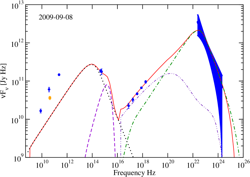
Figure 16: Spectral energy distribution (SEDs) of PKS 0528+134 corresponding the first XMM-Newton observation. Blue points correspond to the observational data. The radio data correspond to the integrated radio flux from single-dish measurements. The orange radio point at 43 GHz is the flux of the VLBA core component. The continuous lines correspond to the best fit for each SED. The dotted line represents the synchrotron spectrum, the dot-dot-dashed line corresponds to the Synchrotron self Compton (SSC), the dot-dashed line is the external radiation Compton (ERC), and the short-dashed line is the disk thermal component.

As a representative example, the fit to the SED of PKS 0528+134 during the first XMM-Newton observation is shown in Figure 16. The parameters used for this particular fit are shown in table 6. The synchrotron (dotted line), synchrotron self Compton (SSC) (dot-dot-dashed line), external radiation Compton (ERC) (dot-dashed line), and the direct disk emission (short-dashed line) components are shown separately, in addition to the total SED fit curve.

Table 6: Parameters used in the fit for the SED of PKS 0528+134 corresponding to the XMM-Newton observation of September 8, 2009 (JD 2455082.94).

Parameter	Value
$\gamma_{min}$	1400
$\gamma_{max}$	$10^{5}$
Injection electron spectral index	3.65
Escape time parameter ($t_{\rm esc}=\eta_{\rm esc}\,R/c$)	$\eta_{\rm esc}=50$
Magnetic field [G]	2.05
Injection height [pc]	$z_{0}=0.13$
Bulk Lorentz factor $\Gamma$	20.4
Accretion disk luminosity [$10^{46}$ erg/s]	$L_{46}=17$
Blob radius [cm]	$1.9\times 10^{16}$
Black hole mass [$M_{\odot}$]	$1.08\times 10^{9}$
Observing angle [degrees]	$\theta_{obs}=3.02$
Doppler factor	$D=19.0$
Redshift	Z = 2.06
$L_{e}$ (jet) [erg/s]	$2.3\times 10^{45}$
$L_{B}$ (jet) [erg/s]	$2.3\times 10^{45}$
$L_{B}/L_{e}$	1.0

We were able to achieve good fits for all four SEDs of PKS 0528+134 in quiescence. Table 7 lists the most relevant parameters used in each fit. Fit parameters close to equipartition could be found for all four SEDs. In general, no obvious correlation between the different parameters was found. However, a strong correlation (Pearson’s correlation coefficient $r\approx 1$) was found between the magnetic field and the optical flux (R-band), reflecting the synchrotron dominance in the optical band.

Table 7: Relevant fit parameters for the SEDs of PKS 0528+134

SED	B [G]	$F_{R}$ [Jy Hz]	$F_{X}$ [erg cm-2 s-1]	$\Gamma$	q	$\eta$	$L_{e}$	$L_{B}$	$L_{B}/L_{e}$	$z_{0}$ [pc]
1	2.05	1.8399e+11	1.6249e-12	20.4	3.65	50	2.30e+45	2.30e+45	1.0	0.13
2	2.06	1.6570e+11	1.3224e-12	20.1	3.85	50	2.39e+45	2.26e+45	0.95	0.13
3	3.7	3.8000e+11	1.3702e-12	17.5	3.7	70	1.18e+45	1.73e+45	1.46	0.11
4	2.21	1.9799e+11	1.4367e-12	21.1	3.65	40.3	2.24e+45	2.40e+45	1.07	0.135

We point out that our model only includes the emission from the blazar zone, assumed here to be on sub-pc scales. It is expected that the radio emission originates in the more extended (pc to kpc scales) jet which is not included in our model. Therefore, our fits under-produce the radio spectra in all SEDs. While most of the radio data shown in Figure 16 are obtained by single-dish instruments and therefore represent the integrated flux over all radio components, we have also included the 43 GHz flux from the VLBA core component on 16 September 2009, just 2 days after the last XMM-Newton observation. Even this core radio flux is under-represented by our model, suggesting that the higher-frequency emission originates on even smaller scales than the radio core.

7 Discussion

As mentioned in the previous section, good fits with a one-zone leptonic SSC + ERC jet model were possible with parameters close to equipartition. Our fit parameters, in particular, the magnetic fields of $B\sim 2$ – 3 G, characteristic electron energies, $\gamma_{\rm min}\sim 10^{3}$, and jet powers of $L_{e}\sim 10^{45}$ erg s^-1, are in rough agreement with the fit results of Mukherjee et al. (1999). However, we need to point out that the model used in Mukherjee et al. (1999) is not precisely the same as used in this paper, as it was based on a time-average of an evolving particle distribution along the jet. Also, Mukherjee et al. (1999) used a different cosmology (a matter-dominated Universe with $q_{0}=0.5$), resulting in a substantially different luminosity distance. Therefore, our results are not directly comparable. We notice that the Fermi LAT $\gamma$-ray spectra of PKS 0528+134 are systematically softer than the photon indices $\Gamma_{\rm ph}\sim 2.2$ – 2.6 found during the EGRET era (Mukherjee et al., 1999). Therefore, our fits to the LAT SEDs require significantly steeper particle spectral indices.

We also need to caution that the model contains a large number of poorly constrained parameters, and in many cases, different parameter combinations might be able to produce similarly acceptable fits. Therefore, conclusions about correlations between model parameters and observables may not be unique.

A similar study of $\gamma$-ray bright blazars in quiescence has recently been published by Abdo et al. (2010b). Those authors observed 5 blazars (PKS 0208-512, Q 0827+243, PKS 1127-145, PKS1510-089, and 3C 454.3) in their low-activity state with Suzaku and Swift in X-rays and optical/UV, and analyzed the simultaneous Fermi-LAT data. All of those blazars showed X-ray continua consistent with a hard ($\Gamma_{\rm ph}\sim 1.5$) single power-law spectrum, in agreement with our XMM-Newton and Suzaku results on PKS 0528+134. The broadband SEDs of all five blazars were dominated by their high-energy ($\gamma$-ray) output, as in PKS 0528+134. In contrast to our XMM-Newton results on PKS 0528+134, three of the five blazars observed by Abdo et al. (2010b) (PKS 0208-512, PKS 1127-145, and PKS 1510-089) did show significant short-term variability on time scales of $\sim 5$ – 10 hr. However, we need to point out that the observations by Abdo et al. (2010b) did not adhere to the strict quiescence criterion required for triggering our PKS 0528+134 campaign (i.e., the Fermi-LAT $\gamma$-ray flux remaining below the lowest EGRET flux or upper limit persistently for at least two weeks, see §1). In fact, some of their targets (in particular, PKS 0208-512, PKS 1510-089, and 3C 454.3) exhibited substantial $\gamma$-ray flux and even $\gamma$-ray flares within just a few days of the Suzaku observations. Therefore, the X-ray variability reported in Abdo et al. (2010b) may not be characteristic of a truly quiescent state of those blazars as investigated in the case of PKS 0528+134 reported in this paper.

In our analysis of optical spectral variability we found a weak anti-correlation between the B-R color and the R-band magnitude. A possible explanation for this softer when brighter trend can be found in the interplay between the two radiation components that contribute photons to the optical flux: the synchrotron component, which is generated in the jet itself, with a steep spectrum, always dominating at low (R-band) frequencies, and slowly varying emission components associated with the accretion disk and the BLR. The direct accretion disk emission is expected to peak in the ultraviolet and may therefore contribute at the blue end of the optical spectrum. In Section 4.2, we have shown that the observed color variability can not be attributed to the contribution from the CIII] and CIV emission lines in the optical spectrum of PKS 0528+134. Therefore, the obvious candidate is direct, thermal accretion disk emission. The suggestive trend of increasing polarization with increasing wavelength lends further support to this hypothesis.

Given the evidence we found for a substantial accretion disk with a luminosity of $L_{D}\sim 1.7\times 10^{47}$ erg s^-1, it is worth investigating whether at least part of the observed X-ray emission may result from Comptonization of soft disk photons in a hot, thermal corona above the accretion disk. In the extreme scenario, in which the entire XMM-Newton spectrum is produced by the corona, Figure 16 illustrates that one would require the energy dissipated in the corona to be of the same order as that dissipated in the optically thick disk. In the case of Comptonization of soft photons with energy far below the X-ray regime, the X-ray spectral index $\Gamma_{\rm ph}\sim 1.6$ can then be translated into a Comptonization parameter $y=16\,\Theta^{2}\,\tau_{T}\,(1+\tau_{T})$, where $\Theta=kT/(m_{e}c^{2})$ is the dimensionless coronal temperature, through

$$\Gamma_{\rm ph}=-{1\over 2}\pm\sqrt{{9\over 4}+{4\over y}}$$ (2)

yielding a value of $y=1.85$. This would imply coronal parameters of $\Theta^{2}\,\tau_{T}\,(1+\tau_{T})=0.116$. However, in order for the X-ray spectrum to be dominated by coronal Compton emission, the jet SSC emission would have to be strongly suppressed compared to the model fits we presented here. This could, in principle, be achieved by the choice of a much larger emission region size $R$. Such a choice might be problematic for two reasons: (1) For $R\gtrsim 1.7\times 10^{16}\,(D/20)$ cm, causality would not allow for variability on time scales of a day or less; (2) as the observed synchrotron emission would require the same magnetic field as chosen in our SED fits, this would result in the energy density in the leptonic particle population being far below equipartition with the magnetic field. While both arguments may not strictly rule out such a scenario, we strongly prefer our fit scenario, close to equipartition, and allowing for $\sim$ day scale variability.

We found that the shortest observed variability occurs at optical wavelengths. In the standard interpretation, this is the region near the high-frequency end of the synchrotron spectrum, emitted by the highest-energy electrons with the shortest radiative cooling time scales. The synchrotron cooling time scale for electrons radiating via synchrotron emission in the V band, is

$$\tau_{\rm sy}^{\rm obs}(V)\approx 2.2\times 10^{4}\,(1+z)^{1/2}\,B_{G}^{-3/2}\,D^{-1/2}\;{\rm s}$$ (3)

Using the redshift of $z=2.07$, a characteristic magnetic field of $B\sim 2$ G, and a typical Doppler factor of $D=19$ from our fit results, we find an observed synchrotron cooling time of $\tau_{\rm sy}^{\rm obs}(V)\approx 0.9$ hr. Since the SED of PKS 0528+134 is strongly dominated by the $\gamma$-ray emission, the actual radiative cooling rate is expected to be shorter than the rate expected from synchrotron emission alone, by a factor corresponding to the Compton dominance (the ratio of power output in the high-energy vs. the synchrotron component), which is of order 10. Therefore, the total radiative cooling time scale of electrons emitting synchrotron in the V band is likely of the order of $\sim 1$ minute or shorter. This suggests that the light curves of variability in all optical bands are strongly dominated by light-travel time effects rather than microphysical (acceleration and cooling) time scales.

The very moderate degree of variability observed in all wavelength bands, in tandem with the short radiative cooling time scales, implies on-going particle acceleration in the quiescent state of PKS 0528+134. On the other hand, the significant polarization variability hints towards a turbulent process. Steady, on-going particle acceleration can be envisioned in shear-layers of radially stratified jets or particle acceleration at standing features, such as re-collimation shocks. However, the magnetic fields in shear-layers of radially stratified jets are expected to be highly ordered due to the directionality of the differential motion in those systems. Therefore, our results seem to favor scenarios involving turbulent acceleration, possibly associated with stationary re-collimation shocks.

Further evidence for turbulent processes comes from our polarization results. A power-law distribution of non-thermal electrons with a spectral index $p$ can produce synchrotron emission with a maximum polarization degree of $P_{s}^{\rm max}=(p+1)/(p+7/3)$ for a perfectly ordered magnetic field (Rybicki & Lightman, 1986). Based on our modeling results in Section 6, the high-energy (cooled) part of the electron spectrum is expected to have a spectral index of $p=q+1\approx 4.6$. This would yield a maximum polarization degree of $P_{s}^{\rm max}\approx 70$ %. The fact that the actual degree of polarization remains below $\sim 10$ % indicates the magnetic field is tangled on size scales much smaller than the size of the emission region. The rapid (day scale), apparently random variation of the degree of polarization and the EVPA seems to indicate a turbulent process resulting in a large number of individual cells with randomly oriented magnetic fields. Monte Carlo simulations (D’Arcangelo, 2010) indicate that for a 100 % chaotic magnetic field (i.e., no ordered field component), 150 turbulence cells result in a degree of polarization of $p=(6\pm 3)$ %, in agreement with the observed values for PKS 0528+134. Given a typical variability time scale in the optical of $\sim 1$ day, the size of individual turbulence cells can be estimated as $R_{\rm cell}\sim c\,\delta t_{\rm var}/(N^{1/3}\,D)\sim 2\times 10^{14}$ cm for a Doppler factor of $D\sim 20$ (see §6) and $N=150$ turbulence cells. Comparing the optical polarization variability to the polarization variability of the radio core (see §5), one can speculate that when the optical polarization is high ($\gtrsim 5$ %), the optical EVPA seems to be more closely aligned with the EVPA of the radio component closest to the radio core.

8 Summary and Conclusions

Over the last two decades PKS 0528+134 has become an important target for multiwavelength observations because of its high luminosity from radio through $\gamma$-rays and the extreme flux and spectral variability that it shows in its flaring states. In this paper, we have presented multiwavelength observations of PKS 0528+134 involving the XMM-Newton, RXTE, Suzaku, and Fermi satellites as well as many ground based radio and optical telescopes. Our main goal was to characterize this $\gamma$-ray loud quasar in a quiescent state to improve the understanding of SEDs and variability patterns of this source, and of blazars in general. The variability analysis of the collected data, and the construction and modeling of four SEDs of this source, yielded the following results:

• No significant short term flux and spectral variability (as determined by data in the core campaign) was found in $\gamma$-rays, X-rays and most radio bands. However, for the same time interval, significant flux variability with $\Delta R\lesssim 1^{\rm mag}$ on time scales of several hours was found in the optical, accompanied by a weak spectral softening with increasing flux. The latter trend may be interpreted as a steady contribution of the accretion disk flux at the blue end of the optical spectrum. Optical spectropolarimetry suggests an increasing degree of polarization towards longer wavelengths, lending further support to the hypothesis of synchrotron emission contributing an increasing fraction of the emission towards the red end of the spectrum.

• Data analysis based on a more extended interval (two months or more) shows no significant $\gamma$-ray flux and spectral index variations, but moderate flux variability in the X-rays ($|\Delta F/F|\sim 50$ %) and at radio ($|\Delta F/F|\lesssim 20$ %) frequencies on time scales of $\sim 1$ – 2 weeks. A comparison between XMM-Newton spectra of 2009 September and the Suzaku spectrum of 2008 September/October suggests that the X-ray spectral index remains stable in the quiescent state of PKS 0528+134 even throughout substantial (factor $\sim 2$ – 3) long-term flux variations.

• We constructed four SEDs of PKS 0528+134 in quiescence. Our results show that even in the quiescent state, the bolometric luminosity of PKS 0528+134 is strongly dominated by its $\gamma$-ray emission, although the $\gamma$-ray spectra are significantly steeper than found during the EGRET era.

• We fitted the four SEDs with a leptonic combined SSC+ERC jet model. In this model, the low energy component is produced by the sum of the synchrotron process in the jet and the disk luminosity, and the high energy emission is due to the sum of the synchrotron self-Compton and the external radiation Compton contributions. Fit parameters close to equipartition were found for all SEDs.

• The moderate variability in most wavelength bands, compared to the expected short radiative cooling time scale, implies the persistence of particle acceleration on long time scales. This may favor acceleration scenarios based on standing features, such as re-collimation shocks.

References

- Abdo et al. (2010a) Abdo, A. A., et al., 2010a, ApJ, 715, 429
- Abdo et al. (2010b) Abdo, A. A., et al., 2010b, ApJ, 716, 835
- Abdo et al. (2010c) Abdo, A. A., et al., 2010c, ApJS, 188, 405
- Acciari et al. (2009) Acciari, V. A., et al., 2009, ApJ, 707, 612
- Agudo et al. (2011) Agudo, I., et al., 2011, ApJ, 726, L13
- Aharonian et al. (2007) Aharonian, F., Akhperjanian, A. G., Bazer-Bachi, A. R., et al., 2007, ApJ, 664, L71
- Albert et al. (2007) Albert, J., et al., 2007, ApJ, 669, 862
- Aller et al. (1985) Aller, H. D., Aller, M. F., Latimer, G. E., & Hodge, P. E. 1985, ApJS, 59, 513
- Anders & Grevesse (1989) Anders, E. and Grevesse N. 1989; Geochimica et Cosmochimica Acta 53, 197.
- Arnaud (1996) Arnaud, K. A. 1996; in ASP Conf. Ser. 101: Astronomical Data Analysis Software and Systems (ADASS) V, 17.
- Atwood et al. (2009) Atwood, W. B., et al., 2009, ApJ, 697, 1071
- Baars et al. (1977) Baars, J. W. M., et al. 1977, A&A, 61, 99
- Bach et al. (2007) Bach, U., et al., 2007, A&A, 464, 175
- Böttcher & Chiang (2002) Böttcher, M. & Chiang, J., 2002, ApJ, 403, 663
- Böttcher (2010) Böttcher, M., 2010, in proc. “Fermi Meets Jansky”, Eds. T. Savolainen, Ed. Ros, R. W. Porcas, J. A. Zensus, p. 41
- Böttcher & Dermer (2010) Böttcher, M., & Dermer, C. D., 2010, ApJ, 711, 445
- Bregman et al. (1985) Bregman, J. N., Glassgold, A. E., Huggins, P. J., & Kinney, A. L. 1985, ApJ, 291, 505
- Britzen et al. (1999) Britzen, S., Witzel, A., Krichbaum, T. P., Quian, S. J., & Campbell, R. M. A&A, 341, 418
- Bromberg & Levinson (2009) Bromberg, O., & Levinson, A., 2009, ApJ, 699, 1274
- Cardelli et al. (1989) Cardelli, J. A., Clayton, G. C., & Mathis, J. S., 1989, ApJ, 345, 245
- D’Arcangelo (2010) D’Arcangelo, F. D., 2010, Ph.D. Thesis, Boston University
- Dermer & Schlickeiser (1993) Dermer, C. D., & Schlickeiser, R., 1993, ApJ, 416, 458
- Dickey & Lockman (1990) Dickey, J. M., & Lockman, F. J., 1990, ARAA, 28, 215
- Dingus et al. (1996) Dingus, B. L., Bertsch D. L., Diegel S. W., et al., 1996, ApJ, 467, 589
- Finke et al. (2008) Finke, J. D., Dermer, C. D., & Böttcher, M., 2008, ApJ, 686, 181
- Francis et al. (1991) Francis, P. J., Hewett, P. C., Foltz, C. B., Chaffee, F. H., Weyman, R. J., & Morris, S. L., 1991, ApJ, 373, 465
- Gabriel et al. (2004) Gabriel, C., Denby, M., Fyfe, D. J. et al. 2004; in ASP Conf. Ser. 314: Astronomical Data Analysis Software and Systems (ADASS) XIII, 759.
- Ghisellini et al. (1999) Ghisellini, G., et al. 1999, A&A, 348, 63
- Gurwell et al. (2007) Gurwell, M.A., Peck, A.B., Hostler, S.R., Darrah, M.R., Katz, C.A., & the SMA Team 2007. ”Monitoring Phase Calibrators at Submillimeter Wavelengths”, From ZMachines to ALMA:(Sub)millimeter Spectroscopy of Galaxies, Charlottesville, VA. ASP Conference Series, Vol. 375, A.J. Baker, J. Glenn, A.I. Harris, J.G. Mangum, and M.S. Yun, eds., p 274.
- Hogerheijde et al. (1995) Hogerheijde, M. R., Geus, E. J., Spaans, M., Langevelde, H. J., & Dishoeck, E. F., 1995, 441, L93
- Hunter et al. (1993) Hunter, S. D., Bertsch, D. L., Dingus, B. L., et al., 1993, ApJ, 409, 134
- Jansen et al. (2001) Jansen, F. et al. 2001; AA, 365, L1.
- Jorstad et al. (2001) Jorstad, S.G., Marscher, A.P., Mattox, J.R., Wehrle, A.E., Bloom, S.D., & Yurchenko, A.V., 2001, ApJS, 134, 181
- Jorstad et al. (2005) Jorstad, S. G., et al. 2005, AJ, 130, 1418
- Jorstad et al. (2010) Jorstad, S. G., et al. 2010, ApJ, 715, 362
- Joshi & Böttcher (2010) Joshi, M., & Böttcher, M., 2010, ApJ, in press
- Kalberla et al. (2005) Kalberla, P. M. W., Burton, W. B., Hartmann, Dap, Arnal, E.M ., Bajaja, E., Morras, R., and Pöppel, W. G. L. 2005; AA, 440, 775.
- Leto et al. (2009) Leto, P., Umana, G., Trigilio, C., et al., 2009, A&A, 507, 1467L
- Lister et al. (2009) Lister, M. L., et al., AJ, 138, 1874
- Liszt & Wilson (1993) Liszt, H. S., & Wilson, R. W., 1993, ApJ, 403, 663
- Marscher & Gear (1985) Marscher, A. P., & Gear, W. K., 1985, ApJ, 298, 114
- Mason et al. (2001) Mason, K. O. et al. 2001; AA, 365, L36.
- Mattox et al. (1996) Mattox, J. R., et al., 1996, ApJ, 461, 396
- Mattox et al. (1997) Mattox, J. R., Schachter, J., Molnar, L., et al., 1997, ApJ, 481, 95
- McNaron-Brown et al. (1995) McNaron-Brown, K., Johnson, W. N., Jung, G. V., et al., 1995, ApJ, 451, 575
- Mimica et al. (2004) Mimica, P., et al., 2004, A&A, 418, 947
- Morrison & McCammon (1983) Morrison, R., & McCammon, D., 1983, ApJ, 270, 119
- Mukherjee et al. (1996) Mukherjee, R., Dingus, B. L., Gear, W. K., et al., et al., 1996, ApJ, 470, 831
- Mukherjee et al. (1999) Mukherjee, R., Böttcher, M., Hartman, R. C., Sreekumar, P., Thompson, D. J., Mahoney, W. A., Pursimo, T., Sillanpää, A., & Takalo, L. O., 1999, ApJ, 527, 132
- Peng et al. (2001) Peng B., et al. 2001, ApJ, 551, 172
- Piner et al. (2006) Piner, B. G., Bhattarai, D., Edwards, P. G., & Jones, D.L., 2006, ApJ, 640, 196
- Pohl et al. (1996) Pohl, M., et al. 1996, A&AS, 120, 529
- Raiteri et al. (1998) Raiteri, C. M., et al. 1998, A&AS, 130, 495
- Raiteri et al. (2007) Raiteri, C. M., et al., 2007, A&A, 473, 819
- Raiteri et al. (2008) Raiteri, C. M., et al., 2008, A&A, 491, 755
- Reich et al. (1993) Reich, W., et al. 1993, A&A, 273, 65
- Rieger & Duffy (2004) Rieger, F. M., & Duffy, P., 2004, ApJ, 617, 155
- Rieger & Duffy (2006) Rieger, F. M., & Duffy, P., 2006, ApJ, 652, 1044
- Rybicki & Lightman (1986) Rybicki, G. B., & Lightman, A. P., 1986, “Radiative Processes in Astrophysics”, Wiley-VCH.
- Sambruna et al. (1997) Sambruna, R. M., et al. 1997, ApJ, 474, 639
- Schlegel et al. (1998) Schelegel, D. J., Finkbeiner, D. P., Davis, M., 1998, ApJ, 500, 525
- Shakura & Sunyaev (1973) Shakura, N. I., & Sunyaev, R. A., 1973, A&A, 24, 337
- Sikora et al. (1994) Sikora, M., Begelman, M. C., & Rees, M. J., 1994, ApJ, 421, 153
- Smith et al. (1985) Smith et al. 1985, AJ, 90, 1184
- Spada et al. (2001) Spada, M., et al., 2001, MNRAS, 325, 1559
- Stawarz & Ostrowski (2002) Stawarz, L., & Ostrowski, M., 2002, ApJ, 578, 763
- Stevens et al. (1994) Stevens, J. A., et al. 1994, ApJ, 437, 91
- Strüder et al. (2001) Strüder, L., Briel, U., Danner, K. et al 2001; AA, 365, L18.
- Teräsranta et al. (1998) Teräsranta, H., Tornikoski, M., Mujunen, A. et al. 1998, A&AS, 132, 305
- Valtaoja & Teräsranta (1995) Valtaoja, E., Teräsranta, H. 1995, A&A, 297, L13
- Wall & Peacock (1985) Wall, J. V., & Peacock, J. A., 1985, MNRAS, 216, 173
- Wardle & Kronberg (1974) Wardle, J. F. C., & Kronberg, P. P., 1974, ApJ, 194, 294
- Yurchenko (2001) Yurchenko, A.V., 2001, ApJS, 134, 181
- Zhang et al. (1994) Zhang Y.F., Marscher A.P., Aller H.D., et al., 1994, ApJ, 432, 91