ADAPTIVE TIME SPLITTING METHOD FOR MULTI-SCALE EVOLUTIONARY PARTIAL DIFFERENTIAL EQUATIONS

Abstract

This paper introduces an adaptive time splitting technique for the solution of stiff evolutionary PDEs that guarantees an effective error control of the simulation, independent of the fastest physical time scale for highly unsteady problems. The strategy considers a second order Strang method and another lower order embedded splitting scheme that takes into account potential loss of order due to the stiffness featured by time-space multi-scale phenomena. The scheme is then built upon a precise numerical analysis of the method and a complementary numerical procedure, conceived to overcome classical restrictions of adaptive time stepping schemes based on lower order embedded methods, whenever asymptotic estimates fail to predict the dynamics of the problem. The performance of the method in terms of control of integration errors is evaluated by numerical simulations of stiff propagating waves coming from nonlinear chemical dynamics models as well as highly multi-scale nanosecond repetitively pulsed gas discharges, which allow to illustrate the method capabilities to consistently describe a broad spectrum of time scales and different physical scenarios for consecutive discharge/post-discharge phases.

AMS Subject Classification: 65G20, 65M15, 65Z05, 65L04, 35K57, 35A35, 35C07

Dedication

Cet article est dédié à la mémoire de Michelle Schatzman. Spécialiste des méthodes de décomposition d’opérateur, sa grande clairvoyance scientifique lui a permis d’orienter plusieurs chercheurs débutants sur ce sujet à un moment où il pouvait sembler achevé. Michelle aimait dire qu’il n’y a pas de frontière entre les branches des mathématiques et que seule une grande culture permet de naviguer dans cette forêt et d’y trouver les bonnes techniques pour résoudre un problème. Ce travail est un hommage; à la croisée des mathématiques et de leur applications effectives, il tente d’illustrer cette assertion. Michelle, ton dynamisme, ton humour et ton plaisir à parler mathématiques nous manquent.

1 Introduction

Numerical simulations of multi-scale phenomena are commonly used for modeling purposes in many applications such as combustion, plasma discharges, chemical vapor deposition or air pollution modeling. In general, all these models raise several difficulties created by the high number of unknowns, the wide range of temporal scales due to large and detailed chemical kinetic mechanisms, as well as steep spatial gradients associated with localized fronts of high chemical activity. In this context, faced with the induced stiffness of these time dependent problems, a high performing numerical strategy for multidimensional simulations considers a time operator splitting with dedicated high order time integration methods for reaction and diffusion problems, in order to exploit efficiently the special features of each problem. Such a numerical strategy for time discretization has been presented in [9] and extended in [8] with multiresolution techniques for adaptive space discretization. The main idea is to use a second order Strang scheme to solve independently reaction and diffusion problems in three successive fractional steps, taking into account that for multi-scale phenomena better performances are usually expected while ending the splitting scheme by the part involving the fastest scales, as it has been proven in [5]. Therefore, based on these theoretical results and on the construction of the splitting solver, this strategy provides an accurate resolution of such stiff problems even for splitting time steps much larger than either the fastest time scales involved in the source terms or the time step restrictions related to spatial grid discretizations.

Up to our days, fixed splitting time step schemes have been largely used in the literature [16, 24, 22], and the relevance of our numerical strategy [9, 8] has been evaluated in the framework of stiff reaction waves for which a constant splitting time step is more than reasonable to precisely describe the global coupling of the split phenomena. However, such a fixed time stepping strategy would surely lead to major difficulties and limitations for problems describing highly non stationary models with very different dynamics such as flame ignition and propagation or repetitively pulsed plasmas discharges [23], all the more in the framework of large scale simulations. It is thus essential to be able to dynamically adapt splitting time steps for the simulation of such multi-scale problems with strongly evolving dynamics.

In order to guarantee a precise description of the coupled multi-scale phenomenon, this splitting time step adaptation strategy must rely on a local error estimate, which can be obtained by considering a lower order embedded method. This is a common practice for ODEs numerical solution [13], which yields very efficient and eventually high order methods for which time steps can dynamically adapt according to a given tolerance, to sufficiently small values in order to cope with the fastest time scales of the problem. However, it is well known that for stiff problems and larger accuracy tolerances, the order of the methods can degenerate, yielding non reliable error estimates and possibly, much larger global errors than expected by the given tolerance. Such a scenario will be all the more valid in the framework of the resolution of PDEs where fine grid and large gradients coupled with stiff source terms lead to especially stiff problems. In particular, our numerical strategy [9, 8] is built in such a way that the main source of error is the splitting error, each building block relying on high order adaptive and dedicated numerical methods; therefore, it is essential not only to construct a reliable splitting error estimate, but also to guarantee an effective error control within the so claimed accuracy tolerance.

In this article, we present a novel strategy to control the local splitting error with two different splitting schemes, the first one is a second order Strang technique whereas the second one considers a shifted Strang formula, built with a $\varepsilon$-shift in time of the classical Strang formula. This second method is embedded because the first substep is common to both methods to reduce computational cost, and inherits from the Strang scheme, stability properties and the same numerical behavior in the context of stiff problems; nevertheless, it is only of order one due to the slightly lack of symmetry. In the first part of the paper, we conduct a complete error estimate of this new splitting method in order to characterize the local error estimate that will be computed out of first and second order splitting resolutions. We define then a domain of application of the adaptive method in which the local error estimates guarantee an effective error control of the solution according to the given tolerance. The key issue is related to the evaluation of a maximum splitting time step, called the critical splitting time step, as a function of $\varepsilon$, for which local error estimates are valid. A numerical validation of the theoretical estimates is performed in the framework of traveling reaction waves for a simple PDE, for which the threshold and critical time steps can be also theoretically estimated and compared with numerical results.

However, in order to extend the numerical strategy to more realistic configurations, for which theoretical evaluation of critical time steps is out of reach, we develop a complementary and general numerical procedure based on numerical estimates, that allows to establish the domain of application of the method by simultaneously choosing the appropriate $\varepsilon$ for a given tolerance. This procedure is tested in the framework of nonlinear chemical dynamics of Belousov-Zhabotinsky (BZ) reactions in a very stiff case in both time and space, yielding satisfactory results. As a consequence, a final numerical strategy is conceived that considers adaptive splitting time steps and that evaluates simultaneously critical time steps as well as best-suited $\varepsilon$, in order to guarantee error control for a given accuracy tolerance of the simulation with splitting time steps as large as possible. The relevance of the proposed strategy is first evaluated for the BZ reaction-diffusion equations, whereas a more complex problem issued from the simulation of multi-pulsed gas discharges involving several dynamics with very different typical time scales, constitutes the second test-case. It is shown that for this second very stiff reaction-diffusion system, splitting time steps can cover a range of three orders of magnitude and always guarantee a proper respect of the prescribed tolerance.

The paper is organized as follows: section 2 describes the adaptive time splitting strategy; in section 3, we perform the numerical analysis of the proposed method and identify the limit of validity of the local error estimate which is at the heart of the adapting procedure. Section 4 is devoted to the validation of the previous theoretical estimates and to a theoretical/numerical study of the critical splitting time steps in the context of a 1D reaction-diffusion problem featuring traveling wave solutions. In section 5 we present the final numerical strategy that includes an additional numerical procedure to evaluate critical time steps and suitable $\varepsilon$. The potential of the method is illustrated for the proposed two test-cases in section 6. We end in the last part with some concluding remarks.

2 Adaptive Time Splitting Method

Let us first set the general mathematical framework of this work. A class of multi-scale phenomena can be modeled by general reaction-diffusion systems of type:

$$\left.\begin{array}[]{ll}\partial_{t}\mathbf{u}-\partial_{\mathbf{x}}\left(\mathbf{D}(\mathbf{u})\partial_{\mathbf{x}}\mathbf{u}\right)=\mathbf{f}\left(\mathbf{u}\right),&\quad\mathbf{x}\in\mathbb{R}^{d},\ t>0,\\[4.30554pt] \mathbf{u}(0,\mathbf{x})=\mathbf{u}_{0}(\mathbf{x}),&\quad\mathbf{x}\in\mathbb{R}^{d},\ t=0,\end{array}\right\}$$ (1)

where $\mathbf{f}:\mathbb{R}^{m}\to\mathbb{R}^{m}$ and $\mathbf{u}:\mathbb{R}\times\mathbb{R}^{d}\to\mathbb{R}^{m}$, with a tensor of order $d\times d\times m$ as diffusion matrix $\mathbf{D}(\mathbf{u})$.

In the following we will focus on the simplified case of linear diagonal diffusion, for which the elements of the diffusion matrix are written as $D_{i_{1}i_{2}i_{3}}(\mathbf{u})=D_{i_{3}}\delta_{i_{1}i_{2}}$ for some positive indices $i_{1}$, $i_{2}$, $i_{3}$, so that the diffusion operator reduces to the heat operator with some scalar diffusion coefficient $D_{i_{3}}$ for component $u_{i_{3}}$ of $\mathbf{u}$. A scalar one-dimensional model is considered in order to simplify the presentation, taking into account that extension into higher dimensions of $\mathbf{x}$ or $\mathbf{u}$ is straightforward:

$$\left.\begin{array}[]{ll}\partial_{t}u-\partial^{2}_{x}u=f(u),&\quad x\in\mathbb{R},\ t>0,\\[4.30554pt] u(0,x)=u_{0}(x),&\quad x\in\mathbb{R},\ t=0,\end{array}\right\}$$ (2)

where $f$ and $u_{0}$ are smooth functions. We denote by $T^{t}u_{0}$ the solution of (2).

Introducing standard decoupling of the diffusion and reaction parts of (2), we denote by $X^{t}u_{0}$ the solution of the diffusion equation:

$$\begin{array}[]{ll}\partial_{t}u_{D}-\partial^{2}_{x}u_{D}=0,&\quad x\in{\mathbb{R}},\ t>0,\end{array}$$ (3)

with initial data $u_{D}(0,\cdot)=u_{0}(\cdot)$ after some time $t$; and by $Y^{t}u_{0}$, the solution of the reaction part where spatial coordinate $x$ can be considered as a parameter:

$$\begin{array}[]{ll}\partial_{t}u_{R}=f(u_{R}),&\quad x\in{\mathbb{R}},t>0,\end{array}$$ (4)

with $u_{R}(0,\cdot)=u_{0}(\cdot)$.

The two Lie approximation formulae of the solution of system (2) are then defined by

$$L^{t}_{1}u_{0}=X^{t}Y^{t}u_{0},\quad L^{t}_{2}u_{0}=Y^{t}X^{t}u_{0},$$ (5)

whereas the two Strang approximation formulae [25, 26] are given by

$$S^{t}_{1}u_{0}=X^{t/2}Y^{t}X^{t/2}u_{0},\quad S^{t}_{2}u_{0}=Y^{t/2}X^{t}Y^{t/2}u_{0}.$$ (6)

It is well known that Lie formulae (5) (resp. Strang formulae (6)) are an approximation of order $1$ (resp. $2$) of the exact solution of (2). Higher order splitting schemes are also possible. Nevertheless, the order conditions for such composition methods state that either negative time substeps or complex coefficients or non convex combinations are necessary [13]. The formers imply usually important stability restrictions and more sophisticated numerical implementations. In the particular case of negative time steps, they are completely undesirable for PDEs that are ill-posed for negative time progression.

An adaptive time stepping strategy is based on a local error estimate which can be obtained by using two schemes of different order, in this case $S^{t}_{1}$ or $S^{t}_{2}$, locally of order $3$, and $L^{t}_{1}$ or $L^{t}_{2}$, locally of order $2$. For instance, the Embedded Split-Step Formulae given in [17] consider $S^{t}_{1}$ and $L^{t}_{2}$ or $S^{t}_{2}$ and $L^{t}_{1}$, noticing that

$$L^{t}_{1}u_{0}=X^{t}Y^{t/2}Y^{t/2}u_{0},$$

where $Y^{t/2}u_{0}$ is also used to compute $S^{t}_{2}u_{0}$. Nevertheless, in the context of multi-scale phenomena, order reductions may appear due to short-life transients associated with the fastest variables when one considers splitting time steps larger than the fastest scales. It has been proved in [5] that better performances are expected while ending the splitting scheme by the part involving the fastest time scales of the phenomenon. In particular, in the case of linear diagonal diffusion problems, no order loss is expected for the $L_{2}^{t}$ and $S_{2}^{t}$ schemes when fast scales are present in the reactive term. Therefore, the embedding procedure must be carefully conceived taking into consideration these theoretical studies.

We introduce a shifted Strang formula

$$S^{t}_{2,\varepsilon}u_{0}=Y^{(1/2-\varepsilon)t}X^{t}Y^{(1/2+\varepsilon)t}u_{0},$$ (7)

locally of order $2$, due to the lack of symmetry, for $\varepsilon$ in $[-1/2,0)\cup(0,1/2]$. In this way, a local error estimate is computed based on two solutions for which orders are guaranteed and a potential loss of order is simultaneous, following

$$\left(\begin{array}[]{c}S^{\Delta t}_{2}u_{0}\\[4.30554pt] S^{\Delta t}_{2,\varepsilon}u_{0}\end{array}\right)=\left(\begin{array}[]{c}Y^{\Delta t/2}X^{\Delta t}Y^{\Delta t/2}u_{0}\\[4.30554pt] Y^{(1/2-\varepsilon){\Delta t}}X^{\Delta t}Y^{(1/2+\varepsilon)\Delta t}u_{0}\end{array}\right),$$ (8)

for some splitting time step $\Delta t>0$. Embedding is accomplished as long as $\varepsilon$ is different from $-1/2$, that is $S^{\Delta t}_{2,\varepsilon}u_{0}$ different from $L^{t}_{2}u_{0}$. On the other hand, if $\varepsilon$ is equal to $1/2$, $S^{\Delta t}_{2,\varepsilon}u_{0}$ is defined as $L^{t}_{1}u_{0}$, which it is not suitable for stiff configurations as it was previously discussed [5]. Therefore, $\varepsilon$ should be contained in $(-1/2,0)\cup(0,1/2)$. Shifted $S^{\Delta t}_{1,\varepsilon}u_{0}$ is defined in a similar way and depending on the multi-scale character of the problem, it might be the appropriate choice along with $S^{\Delta t}_{1}u_{0}$.

Taking into account that

$$S^{\Delta t}_{2}u_{0}-S^{\Delta t}_{2,\varepsilon}u_{0} = S^{\Delta t}_{2}u_{0}-T^{\Delta t}u_{0}+T^{\Delta t}u_{0}-S^{\Delta t}_{2,\varepsilon}u_{0},$$ (9)

$$= \mathcal{O}(\Delta t^{3})+\mathcal{O}(\Delta t^{2})\approx\mathcal{O}(\Delta t^{2}),$$

for a given accuracy tolerance $\eta$,

$$\big{\|}S^{\Delta t}_{2}u_{0}-S^{\Delta t}_{2,\varepsilon}u_{0}\big{\|}<\eta$$ (10)

must be verified in order to accept current computation with $\Delta t$, while new time step is calculated by

$$\Delta t^{\rm new}=\upsilon\,\Delta t\sqrt{\frac{\eta}{\big{\|}S^{\Delta t}_{2}u_{0}-S^{\Delta t}_{2,\varepsilon}u_{0}\big{\|}}},$$ (11)

with security factor $0<\upsilon\leq 1$ close to one. This comes from a classical adaptive time stepping procedure for stiff ODEs solution, for which more sophisticated formulae than (11) can be also considered, see [14] for example.

The error control of these adaptive methods is fully guaranteed as long as the orders of both, the main and the embedded integration methods, remains valid. This is the case for small enough time steps for which asymptotic theoretical estimates hold, but remains an open problem for larger time steps for which the validity of the formers is assumed. This is a key point in this work, because we propose not only a new splitting strategy with adaptive time steps as described in this section, but we aim also at applications for which splitting time steps may go beyond the fastest scales associated with each subproblem in order to obtain important computational savings. Therefore, a technique that guarantees consistently error control for all possible separation scales must be pursued, but first of all, a detailed numerical analysis of the method must be performed. This is the goal of the following part.

3 Numerical Analysis of the Method

In this part, we develop the numerical analysis of the proposed method. It is mainly based on the theoretical study of the introduced shifted Strang formula (7) and the domain of validity of the local error estimates. However, first of all, we introduce the Lie formalism which will be used as mathematical tool of analysis.

3.1 The Lie operator formalism

We introduce the Lie operator formalism in order to generalize the exponential of a linear operator in the context of nonlinear operators. Let $X$ be a Banach space, $T_{0}>0$ and $F$, an unbounded nonlinear operator from $D(F)\subset X$ to $X$, we consider the general autonomous equation:

$$\left.\begin{array}[]{ll}{\displaystyle u^{\prime}(t)=F(u(t)),}&\quad 0<t<T_{0},\\[4.30554pt] u(0)=u_{0},&\quad t=0.\end{array}\right\}$$ (12)

The exact solution of this evolutionary equation is (formally) given by

$$u(t)=T^{t}u_{0},\quad 0\leq t\leq T_{0}$$ (13)

where $T^{t}$ is the semiflow associated with (12); in particular we can set $F(u)=\partial^{2}_{x}u+f(u)$ as in (2). The Lie operator $D_{F}$ associated with $F$ is then a linear operator acting on the space of operators defined in $X$ [13, 6]. More precisely, for any unbounded nonlinear operator $G$ from $D(G)\subset X$ to $X$ with Fréchet derivative $G^{\prime}$, $D_{F}$ maps $G$ into a new operator $D_{F}G$, such that for any $v$ in $X$:

$$(D_{F}G)(v)=G^{\prime}(v)F(v).$$ (14)

Hence, by induction on $n$ with solution $u$ of (12), we obtain

$$\frac{\partial^{n}}{\partial t^{n}}G(u(t))=(D^{n}_{F}G)(u(t)),$$

and a formal Taylor expansion yields

$$G(u(t))=\sum_{n=0}^{+\infty}\frac{t^{n}}{n!}\left(\frac{\partial^{n}}{\partial t^{n}}G(u(t))\right)\bigg{|}_{t=0}=\left(\sum_{n=0}^{+\infty}\frac{t^{n}}{n!}D^{n}_{F}G\right)u_{0}=\left(e^{tD_{F}}G\right)u_{0}.$$ (15)

If we now assume that $G$ is the identity operator Id, we obtain

$$u(t)=T^{t}u_{0}=\left(e^{tD_{F}}\textrm{Id}\right)u_{0}.$$

Therefore, the Lie operator is indeed a way to write the solution of a nonlinear equation in terms of a linear but differential operator. Following (15), an important result obtained by Gröbner in 1960 [12], considers the composition of two semiflows $T_{1}^{t}$ and $T_{2}^{s}$ associated with $F_{1}$ and $F_{2}$ for any $v$ in $X$:

$$T_{1}^{t}T_{2}^{s}v=\left(e^{sD_{F_{2}}}T_{1}^{t}\right)v=\left(e^{sD_{F_{2}}}e^{tD_{F_{1}}}\textrm{Id}\right)v.$$

3.2 Error analysis

In this paragraph, we conduct the error analysis of the approximation of $T^{t}$ by $S^{t}_{2,\varepsilon}$ in a linear framework. Then, we extend these results to a general nonlinear configuration given by problem (2), using the Lie operator formalism. General estimates for the approximation of $T^{t}$ by $S_{2}^{t}$ are also drawn. We end in the last part with a mathematical study that shows the domain of application of the method described in $\S~{}$2, for which an effective error control is guaranteed within an accuracy tolerance. To simplify the notations in what follows, we will denote $S_{2}^{t}$ by $S^{t}$ and $S^{t}_{2,\varepsilon}$ by $S^{t}_{\varepsilon}$.

Assume that $A$ and $B$ are linear bounded operators and define

$$S^{t}_{\varepsilon}u_{0}=e^{(1/2-\varepsilon)tA}e^{tB}e^{(1/2+\varepsilon)tA}u_{0}$$

as an approximation of $e^{t(A+B)}$. The following theorem gives the expansion in powers of $t$ of the difference between $e^{t(A+B)}$ and $S^{t}_{\varepsilon}$. We recall the definition of the brackets between $A$ and $B$: $[A,B]=AB-BA$.

Theorem 3.1.

Assume that $A$ and $B$ are linear bounded operators, for $t$ and $\varepsilon$ small enough, the following asymptotic holds

$$e^{t(A+B)}u_{0}-S^{t}_{\varepsilon}u_{0}=-\varepsilon t^{2}[A,B]u_{0}+\frac{t^{3}}{24}(\big{[}A,[A,B]\big{]}+2\big{[}B,[A,B]\big{]})u_{0}+\mathcal{O}(\varepsilon t^{3})+\mathcal{O}(t^{4}).$$

Proof 3.2.

Proof is straightforward by using the Taylor formula with integral remainder for a linear bounded operator $A$:

$$e^{tA}=\text{Id}+tA+\frac{t^{2}A^{2}}{2}+\frac{t^{3}A^{3}}{6}+\int_{0}^{t}\frac{(t-s)^{3}}{6}A^{4}e^{sA}\,{\rm d}s.$$

We extend now the previous theorem to our nonlinear framework given by (2). In order to do this, we introduce the spaces $C^{\infty}({\mathbb{R}})$ of functions of class $C^{\infty}$ on ${\mathbb{R}}$, and $C^{\infty}_{b}({\mathbb{R}})$ of functions of class $C^{\infty}$ on ${\mathbb{R}}$ and bounded over ${\mathbb{R}}$. We consider also the Schwartz space $\mathcal{S}({\mathbb{R}})$ defined by

$$\mathcal{S}\left(\mathbb{R}\right)=\{g\in C^{\infty}(\mathbb{R})\mid\sup_{v\in\mathbb{R}}|v^{\alpha_{1}}\partial_{v}^{\alpha_{2}}g(v)|<\infty\quad\,\textrm{for\,all\,integers}\,\alpha_{1},\alpha_{2}\};$$

and we define the space $\mathcal{S}_{1}({\mathbb{R}})$, made out of functions $v$ belonging to $C^{\infty}_{b}({\mathbb{R}})$ such that $v^{\prime}$ belongs to $\mathcal{S}({\mathbb{R}})$. Let us consider now equation (2) and give the expansion in powers of $t$ of the difference between $T^{t}$ and $S^{t}_{\varepsilon}$, given by (7).

Theorem 3.3.

Assume that $u_{0}$ belongs to $\mathcal{S}_{1}\left(\mathbb{R}\right)$ and that $f$ belongs to $C^{\infty}({\mathbb{R}})$. For $t$ and $\varepsilon$ small enough, the following asymptotic holds

$$T^{t}u_{0}-S^{t}_{\varepsilon}u_{0} = -\varepsilon t^{2}f^{\prime\prime}(u_{0})\left(\frac{\partial u_{0}}{\partial x}\right)^{2}$$ (16)

$$+\frac{t^{3}}{24}(f^{\prime}(u_{0})f^{\prime\prime}(u_{0})+f(u_{0})f^{(3)}(u_{0}))\left(\frac{\partial u_{0}}{\partial x}\right)^{2}$$

$$-\frac{t^{3}}{12}f^{(4)}(u_{0})\left(\frac{\partial u_{0}}{\partial x}\right)^{4}-\frac{t^{3}}{3}f^{(3)}(u_{0})\left(\frac{\partial u_{0}}{\partial x}\right)^{2}\frac{\partial^{2}u_{0}}{\partial x^{2}}$$

$$-\frac{t^{3}}{6}f^{\prime\prime}(u_{0})\left(\frac{\partial^{2}u_{0}}{\partial x^{2}}\right)^{2}+\mathcal{O}(\varepsilon t^{3})+\mathcal{O}(t^{4}).$$

Proof 3.4.

We introduce the two Lie operators $D_{\Delta}$ and $D_{f}$ associated with $\partial^{2}_{x}$ and $f$ and write

$$T^{t}u_{0}-S^{t}_{\varepsilon}u_{0}=\left(e^{t(D_{\Delta}+D_{f})}\rm{Id}\right)u_{0}-\left(e^{(1/2+\varepsilon)tD_{f}}e^{tD_{\Delta}}e^{(1/2-\varepsilon)tD_{f}}\rm{Id}\right)u_{0}.$$

With Theorem 3.1 we can deduce that

$$T^{t}u_{0}-S^{t}_{\varepsilon}u_{0} = -\varepsilon t^{2}\left([D_{f},D_{\Delta}]\rm{Id}\right)u_{0}+\frac{t^{3}}{24}\left(\big{[}D_{f},[D_{f},D_{\Delta}]\big{]}\rm{Id}\right)u_{0}$$ (17)

$$+\frac{t^{3}}{12}\left(\big{[}D_{\Delta},[D_{f},D_{\Delta}]\big{]}\rm{Id}\right)u_{0}+\mathcal{O}(\varepsilon t^{3})+\mathcal{O}(t^{4}).$$

We are not interested in giving the exact form of the terms $\mathcal{O}(\varepsilon t^{3})$ and $\mathcal{O}(t^{4})$, but these terms can be computed following the same technique developed in [6]. For the term in $\mathcal{O}(t^{2})$, we have by definition and with (14),

$$\left([D_{f},D_{\Delta}]\rm{Id}\right)u_{0} = \left(D_{f}(D_{\Delta}\mathrm{Id})-D_{\Delta}(D_{f}\rm{Id})\right)u_{0},$$

$$= (D_{\Delta}\mathrm{Id})^{\prime}(u_{0})f(u_{0})-(D_{f}\mathrm{Id})^{\prime}(u_{0})\frac{\partial^{2}u_{0}}{\partial x^{2}},$$

$$= \frac{\partial^{2}}{\partial x^{2}}\left(f(u_{0})\right)-f^{\prime}(u_{0})\frac{\partial^{2}u_{0}}{\partial x^{2}}.$$

The last term is by definition the Lie bracket between $\partial^{2}_{x}$ and $f$, a simple computation shows that

$$\frac{\partial^{2}f(u_{0})}{\partial x^{2}}-f^{\prime}(u_{0})\frac{\partial^{2}u_{0}}{\partial x^{2}} = f^{\prime\prime}(u_{0})\left(\frac{\partial u_{0}}{\partial x}\right)^{2}+f^{\prime}(u_{0})\frac{\partial^{2}u_{0}}{\partial x^{2}}-f^{\prime}(u_{0})\frac{\partial^{2}u_{0}}{\partial x^{2}},$$

$$= f^{\prime\prime}(u_{0})\left(\frac{\partial u_{0}}{\partial x}\right)^{2}.$$

Furthermore,

$$\left(\big{[}D_{f},[D_{f},D_{\Delta}]\big{]}\rm{Id}\right)(u_{0})=(f^{\prime}(u_{0})f^{\prime\prime}(u_{0})+f(u_{0})f^{(3)}(u_{0}))\left(\frac{\partial u_{0}}{\partial x}\right)^{2}$$

and

$$\left(\big{[}D_{\Delta},[D_{f},D_{\Delta}]\big{]}\rm{Id}\right)u_{0} = -f^{(4)}(u_{0})\left(\frac{\partial u_{0}}{\partial x}\right)^{4}-4f^{(3)}(u_{0})\left(\frac{\partial u_{0}}{\partial x}\right)^{2}\frac{\partial^{2}u_{0}}{\partial x^{2}}$$

$$-2f^{\prime\prime}(u_{0})\left(\frac{\partial^{2}u_{0}}{\partial x^{2}}\right)^{2}.$$

All the terms are now computed and this concludes the proof of Theorem 3.3.

For $\varepsilon=0$, the next corollary follows directly.

Corollary 3.5.

Assume that $u_{0}$ belongs to $\mathcal{S}_{1}\left(\mathbb{R}\right)$ and that $f$ belongs to $C^{\infty}({\mathbb{R}})$. For $t$ small enough, the following asymptotic holds

$$T^{t}u_{0}-S^{t}u_{0} = \frac{t^{3}}{24}(f^{\prime}(u_{0})f^{\prime\prime}(u_{0})+f(u_{0})f^{(3)}(u_{0}))\left(\frac{\partial u_{0}}{\partial x}\right)^{2}$$ (18)

$$-\frac{t^{3}}{12}f^{(4)}(u_{0})\left(\frac{\partial u_{0}}{\partial x}\right)^{4}-\frac{t^{3}}{3}f^{(3)}(u_{0})\left(\frac{\partial u_{0}}{\partial x}\right)^{2}\frac{\partial^{2}u_{0}}{\partial x^{2}}$$

$$-\frac{t^{3}}{6}f^{\prime\prime}(u_{0})\left(\frac{\partial^{2}u_{0}}{\partial x^{2}}\right)^{2}+\mathcal{O}(t^{4}).$$

From (16) and (18), we can see that

$$S^{t}u_{0}-S^{t}_{\varepsilon}u_{0}=\varepsilon t^{2}f^{\prime\prime}(u_{0})\left(\frac{\partial u_{0}}{\partial x}\right)^{2}+\mathcal{O}(\varepsilon t^{3}),$$ (19)

and thus,

$$T^{t}u_{0}-S^{t}_{\varepsilon}u_{0}=\underbrace{T^{t}u_{0}-S^{t}u_{0}}_{\mathcal{O}(t^{3})}+\underbrace{S^{t}u_{0}-S^{t}_{\varepsilon}u_{0}}_{\mathcal{O}(\varepsilon t^{2})}.$$ (20)

Therefore, we are sure that the real local error of the method, $T^{t}u_{0}-S^{t}u_{0}$, will be bounded by the local error estimate, $err=S^{t}u_{0}-S^{t}_{\varepsilon}u_{0}$, when for a given $\varepsilon$,

$$T^{t}u_{0}-S^{t}_{\varepsilon}u_{0}\approx\mathcal{O}(t^{2})$$ (21)

is verified into (20); that is, when the embedded method is really of lower order as it was assumed in (9). This will be always verified for small enough time steps $t$, for which $T^{t}u_{0}-S^{t}u_{0}\approx\mathcal{O}(t^{3})<err\approx\mathcal{O}(\varepsilon t^{2})$ is guaranteed. Nevertheless, for larger time steps, $err$ will fail to properly predict $T^{t}u_{0}-S^{t}u_{0}$ since we will eventually have $T^{t}u_{0}-S^{t}u_{0}\approx\mathcal{O}(t^{3})>err\approx\mathcal{O}(\varepsilon t^{2})$. When this happens, (21) is no longer true and the previous estimates show that we will rather have $T^{t}u_{0}-S^{t}_{\varepsilon}u_{0}\approx\mathcal{O}(t^{3})$, and assumption (9) will no longer hold.

In order to overcome this difficulty, we must therefore estimate a critical time step $t^{\star}>0$ such that for all $t$ in $[0,t^{*}]$, (21) is guaranteed for a given $\varepsilon$. This will imply that Strang local error, $T^{t}u_{0}-S^{t}u_{0}$, will be indeed bounded by the local error estimate, $err$, and that an effective error control will be achieved for $err$ smaller than a given accuracy tolerance $\eta$. Finally, a suitable choice of $\varepsilon$ can be also made since $t^{\star}$ is related to $\varepsilon$ following (20).

A natural strategy to predict this critical $t^{\star}$ will rely on the previous theoretical estimates and on a more precise knowledge of the structure of the solutions of the PDEs; this is for instance illustrated in the next part in the context of traveling wave solutions.

4 Application to Reaction Traveling Waves

In this part, we will confront the previous theoretical study to a simple reaction diffusion problem that admits self-similar traveling wave solutions such as the KPP equation [18]. The main advantages of considering this kind of problems are that analytic solutions exist and that the featured stiffness can be tuned using a space-time scaling. Therefore, it provides a first numerical validation of the numerical estimates of the method and an evaluation of its domain of application; and on the other hand, a detailed study can be conducted on the impact of the stiffness featured by propagating fronts with steep spatial gradients.

In what follows, we recast previous estimates in the context of these reaction traveling waves, to then deduce an estimate of the time step $t^{\star}$ that defines the limit of application of the method for which local error estimates yield effective error control. We end with a numerical validation of the theoretical results in the context of the resolution of KPP model.

4.1 Numerical estimates

We are interested in the propagation of self-similar waves modeled by parabolic PDEs of type:

$$\left.\begin{array}[]{ll}\partial_{t}u-D\,\partial^{2}_{x}u=kf(u),&\quad x\in\mathbb{R},\ t>0,\\[4.30554pt] u(0,x)=u_{0}(x),&\quad x\in\mathbb{R},\ t=0,\end{array}\right\}$$ (22)

with solution $u(x,t)=u_{0}(x-ct)$, where $c$ is the steady speed of the wavefront, and $D$ and $k$ stand respectively for diffusion and reaction coefficients.

Considering Theorem 3.3 we obtain the following estimate for system (22).

Corollary 4.1.

Assume that $u_{0}$ belongs to $\mathcal{S}_{1}\left(\mathbb{R}\right)$ and that $f$ belongs to $C^{\infty}({\mathbb{R}})$. For $t$ and $\varepsilon$ small enough, the following asymptotic holds

$$T^{t}u_{0}-S^{t}_{\varepsilon}u_{0} = -\varepsilon kDt^{2}f^{\prime\prime}(u_{0})\left(\frac{\partial u_{0}}{\partial x}\right)^{2}$$ (23)

$$+\frac{k^{2}Dt^{3}}{24}(f^{\prime}(u_{0})f^{\prime\prime}(u_{0})+f(u_{0})f^{(3)}(u_{0}))\left(\frac{\partial u_{0}}{\partial x}\right)^{2}$$

$$-\frac{kD^{2}t^{3}}{12}f^{(4)}(u_{0})\left(\frac{\partial u_{0}}{\partial x}\right)^{4}-\frac{kD^{2}t^{3}}{3}f^{(3)}(u_{0})\left(\frac{\partial u_{0}}{\partial x}\right)^{2}\frac{\partial^{2}u_{0}}{\partial x^{2}}$$

$$-\frac{kD^{2}t^{3}}{6}f^{\prime\prime}(u_{0})\left(\frac{\partial^{2}u_{0}}{\partial x^{2}}\right)^{2}+\mathcal{O}(\varepsilon t^{3})+\mathcal{O}(t^{4}).$$

Proof 4.2.

Proof follows directly from demonstration of Theorem 3.3, using (17) and considering that

$$[D_{kf},D_{D\Delta}] = kD[D_{f},D_{\Delta}],$$

$$\big{[}[D_{kf},D_{D\Delta}],D_{D\Delta}\big{]} = kD^{2}\big{[}[D_{f},D_{\Delta}],D_{\Delta}\big{]},$$

$$\big{[}[D_{kf},D_{D\Delta}],D_{kf}\big{]} = k^{2}D\big{[}[D_{f},D_{\Delta}],D_{f}\big{]},$$

where $D_{D\Delta}$ and $D_{kf}$ are the Lie operators associated with $D\partial^{2}_{x}$ and $kf$.

On the other hand, if we now consider system (22) with $k=1$ and $D=1$, the following corollary establishes $t^{*}>0$ such that for all $t$ in $[0,t^{*}]$ (21) is guaranteed for a given $\varepsilon$.

Corollary 4.3.

Assume that $u_{0}$ belongs to $\mathcal{S}_{1}\left(\mathbb{R}\right)$ and that $f$ belongs to $C^{\infty}({\mathbb{R}})$. For a given $\varepsilon$ small enough , define

$$M_{1}=\left\|f^{\prime\prime}(u_{0})\left(\frac{\partial u_{0}}{\partial x}\right)^{2}\right\|_{L^{2}}$$ (24)

and

$$M_{2} =\Biggl{\|} \frac{f^{\prime}(u_{0})f^{\prime\prime}(u_{0})+f(u_{0})f^{(3)}(u_{0})}{24}\left(\frac{\partial u_{0}}{\partial x}\right)^{2}-\frac{f^{(4)}(u_{0})}{12}\left(\frac{\partial u_{0}}{\partial x}\right)^{4}$$ (25)

$$-\frac{f^{(3)}(u_{0})}{3}\left(\frac{\partial u_{0}}{\partial x}\right)^{2}\frac{\partial^{2}u_{0}}{\partial x^{2}}-\frac{f^{\prime\prime}(u_{0})}{6}\left(\frac{\partial^{2}u_{0}}{\partial x^{2}}\right)^{2}\Biggr{\|}_{L^{2}},$$

define $t^{\star}$ by

$$t^{\star}M_{2}=\varepsilon M_{1}.$$ (26)

For all $t$ such that $0<t\leq t^{\star}$ then

$$\|T^{t}u_{0}-S^{t}_{\varepsilon}u_{0}\|_{L^{2}}\approx\mathcal{O}(t^{2}).$$

In a general case, if evaluation of the derivatives of $u_{0}$ and $f$ is feasible, it is then possible to predict the domain of application of the method, $[0,t^{\star}]$, for a given $\varepsilon$ based on the previous result. In the particular case of traveling wave solutions for (22), diffusion and reaction coefficients, $D$ and $k$, might be seen as scaling coefficients in time and space. A dimensionless analysis of a traveling wave, as shown in [11], can be then conducted considering a dimensionless time $\tau$ and a dimensionless space $r$ with

$$\tau=kt\quad\text{and}\quad r=(k/D)^{1/2}x.$$

This analysis allows to find a steady velocity of the wavefront,

$$c=x_{t}\propto(Dk)^{1/2},$$ (27)

whereas the sharpness of the wave profile is measured by

$$\left.{u}_{x}\right|_{\max}\propto(k/D)^{1/2}.$$ (28)

Therefore, condition $Dk=1$ implies constant velocity for all $k=1/D$ but greater $k$ (or smaller $D$) implies higher spatial gradients, and thus, stiffer configurations.

This study gives complementary information on the solution of (22) and in particular, when condition $Dk=1$ is satisfied, it allows to deduce from Corollary 4.3:

$$kt^{\star}M_{2}=\varepsilon M_{1},$$ (29)

with $M_{1}$ and $M_{2}$ given by (24) and (25). Therefore, stiffer configurations given by the presence of steeper spatial gradients will restrain the application domain of the method, according to (29). Nevertheless, for larger gradients, smaller time steps are also required for a given level of accuracy and hence, we can expect a simultaneous reduction of both critical and accurate splitting time steps.

4.2 Numerical illustration: KPP equation

Let us recall the Kolmogorov-Petrovskii-Piskunov model. In their original paper [18], these authors introduced a model describing the propagation of a virus and the first rigorous analysis of a stable traveling wave solution of a nonlinear reaction-diffusion equation [11]. The equation is the following:

$$\partial_{t}u-D\,\partial^{2}_{x}u=k\,u^{2}(1-u),$$ (30)

with homogeneous Neumann boundary conditions. We consider a 1D discretization with $5001$ points on a $[-70,70]$ region for which we have negligible spatial discretization errors with respect to the ones coming from the numerical time integration.

The description of the dimensionless model and the structure of the exact solution can be found in [11] where the dimensionless analysis shows that in the case of $D=1$ and $k=1$, the velocity of the self-similar traveling wave is $c=1/\sqrt{2}$ and the maximal gradient value reaches $1/\sqrt{32}$. The key point of this illustration is that the velocity of the traveling wave is proportional to $(k\,D)^{1/2}$, whereas the maximal gradient is proportional to $(k/D)^{1/2}$. Hence, we consider the case $kD=1$ for which one may obtain steeper gradients for the same speed of propagation.

Throughout all this paper, exact solution $T^{t}u_{0}$ will be approximated by the resolution of the coupled reaction-diffusion problem performed by the Radau5 method [15] with fine tolerances, $\eta_{Radau5}=10^{-10}$. This solution will be referred as the reference or quasi-exact solution. Strang approximations $S^{t}u_{0}$ and $S^{t}_{\varepsilon}u_{0}$ will be computed with a splitting technique recently introduced [8, 9], which considers Radau5 [15] to solve locally point by point the reaction term; and the ROCK4 method [1] for the diffusion problem. Radau5 [15] is a fifth order implicit Runge-Kutta method exhibiting A- and L-stability properties to efficiently solve stiff systems of ODEs, whereas ROCK4 [1] is formally a fourth order stabilized explicit Runge-Kutta method with extended stability domain along the negative real axis, well suited to numerically treat mildly stiff elliptic operators. Both methods implement adaptive time stepping techniques to guarantee computations within a prescribed accuracy tolerance. In order to properly discriminate the previously estimated splitting errors from those coming from temporal integration of the substeps, we consider also fine tolerances, $\eta_{\rm Radau5}=\eta_{\rm ROCK4}=10^{-10}$.

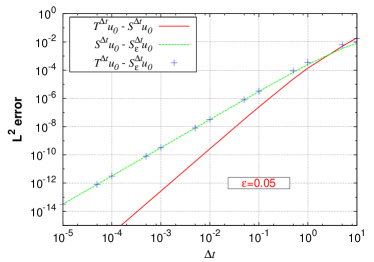
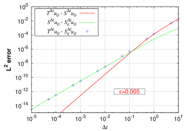
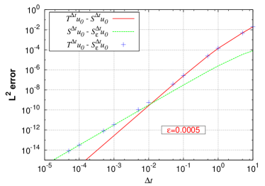
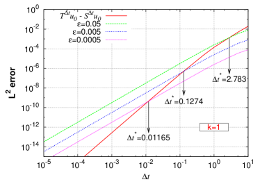
Figure 1: KPP equation with $k=1$. Local $L^{2}$ errors for several splitting time steps $\Delta t$ and $\varepsilon=0.05$ (top left), $0.005$ (top right) and $0.0005$ (bottom left). Bottom right: critical splitting time steps $\Delta t^{\star}$ obtained when $\|T^{\Delta t}u_{0}-S^{\Delta t}u_{0}\|_{L^{2}}\approx\|S^{\Delta t}u_{0}-S^{\Delta t}_{\varepsilon}u_{0}\|_{L^{2}}$ in the numerical tests.

Figures 1 and 2 show $L^{2}$ errors between $T^{t}u_{0}$, $S^{t}u_{0}$ and $S^{t}_{\varepsilon}u_{0}$ solutions for $k=1$, $k=10$ and $k=100$ respectively, and several $\varepsilon$. Notice that estimates (16), (18) and (19) for all three errors in (20) are verified and in particular, for $\Delta t$ larger than critical $\Delta t^{\star}$, the estimated error $err=\|S^{\Delta t}u_{0}-S^{\Delta t}_{\varepsilon}u_{0}\|_{L^{2}}$ is no longer predicting the real local error given by $T^{t}u_{0}-S^{t}u_{0}$.

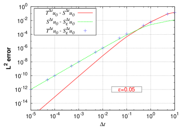
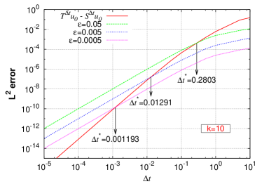
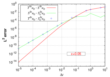
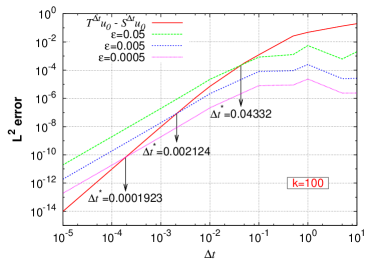
Figure 2: KPP equation with $k=10$ (top) and $k=100$ (bottom). Local $L^{2}$ errors for several splitting time steps $\Delta t$ and $\varepsilon=0.05$ (left). Right: critical splitting time steps $\Delta t^{\star}$ obtained when $\|T^{\Delta t}u_{0}-S^{\Delta t}u_{0}\|_{L^{2}}\approx\|S^{\Delta t}u_{0}-S^{\Delta t}_{\varepsilon}u_{0}\|_{L^{2}}$ in the numerical tests.

With these results, we can also compare real $\Delta t^{\star}$, obtained when $\|T^{\Delta t}u_{0}-S^{\Delta t}u_{0}\|_{L^{2}}\approx\|S^{\Delta t}u_{0}-S^{\Delta t}_{\varepsilon}u_{0}\|_{L^{2}}$ in the numerical tests, with theoretically estimated $\Delta t^{\star}$ following (29). Table 1 summarizes these results where computation of estimated $\Delta t^{\star}$ in (29) is given by the computation of $M_{1}$ and $M_{2}$ with Maple^© according to (24) and (25). A really good agreement can be observed even though theoretical results underestimate the real values. The loss of order depicted by the numerical results, is due to the influence of spatial gradients in the solution, as it was proven in [3]. This explains the error of the predicted critical $\Delta t^{\star}$ in (29) whenever one gets close to the order loss region.

Numerical results show also that $\|S^{\Delta t}u_{0}-S^{\Delta t}_{\varepsilon}u_{0}\|_{L^{2}}\propto\varepsilon$ according to (19) and consequently, $\Delta t^{\star}\propto\varepsilon$; therefore, the working region or domain of application of the method, $\Delta t<\Delta t^{\star}$, depends directly on the choice of $\varepsilon$ as it can be seen in Table 1. Finally, in the context of traveling waves, these numerical experiments show that $\Delta t^{\star}\propto k^{-1}\propto 1/\|\partial u_{0}/\partial x\|_{\infty}$ according to Table 1; hence, application domains are reduced for stiffer configurations but numerical results show also that smaller time steps are required for the same level of accuracy. These conclusions are easily extrapolated to more general self-similar propagating waves.

Table 1: KPP equation. Comparison between real $\Delta t^{\star}_{\mathrm{real}}$, obtained when $\|T^{\Delta t}u_{0}-S^{\Delta t}u_{0}\|_{L^{2}}\approx\|S^{\Delta t}u_{0}-S^{\Delta t}_{\varepsilon}u_{0}\|_{L^{2}}$ in the numerical tests, and theoretically estimated $\Delta t^{\star}_{\mathrm{est}}$ following (29).

		$\varepsilon=0.05$	$\varepsilon=0.005$	$\varepsilon=0.0005$
$k=1$	$\Delta t^{\star}_{\mathrm{real}}$	$2.783$	$0.1274$	$1.17\times 10^{-2}$
	$\Delta t^{\star}_{\mathrm{est}}$	$1.107$	$0.1107$	$1.11\times 10^{-2}$
$k=10$	$\Delta t^{\star}_{\mathrm{real}}$	$0.2803$	$1.29\times 10^{-2}$	$1.19\times 10^{-3}$
	$\Delta t^{\star}_{\mathrm{est}}$	$0.1107$	$1.11\times 10^{-2}$	$1.11\times 10^{-3}$
$k=100$	$\Delta t^{\star}_{\mathrm{real}}$	$4.33\times 10^{-2}$	$2.12\times 10^{-3}$	$1.92\times 10^{-4}$
	$\Delta t^{\star}_{\mathrm{est}}$	$1.11\times 10^{-2}$	$1.11\times 10^{-3}$	$1.11\times 10^{-4}$

5 Construction of the Numerical Strategy

We have presented in $\S~{}$2, a time adaptive numerical scheme fully based on theoretical error estimates developed in $\S~{}$3. We have also studied the necessary general conditions in order to guarantee an effective error control based on local error estimates. In particular, this has been shown in the case of reaction traveling waves in $\S~{}$4, for which theoretical studies give us some insight into the PDE solution. Nevertheless, this is not always possible and it is usually difficult to carry out such kind of analysis for more realistic models. Therefore, based on the theoretical analysis and previous illustrations on the influence of the various parameters of the scheme, a general numerical procedure that completes the adaptive scheme defined in $\S~{}$2, is introduced in the following.

In a first part, we will settle the theoretical framework and the numerical procedure needed to estimate $t^{\star}$, and to define the appropriate $\varepsilon$. This will be illustrated by numerical tests performed on a more complex model of time-space stiff propagating waves. These theoretical and numerical studies will allow to define, at the end, a final numerical strategy.

5.1 Numerical procedure to estimate critical $t^{\star}$ and $\varepsilon$

Let us consider general system (2), based on theoretical estimates (18) and (19), we can write

$$S^{\Delta t}u_{0}-T^{\Delta t}u_{0}=C_{0}\Delta t^{3},$$ (31)

where $C_{0}=C_{1}(u_{0})+\mathcal{O}(\Delta t^{4})$, and

$$S^{\Delta t}u_{0}-S^{\Delta t}_{\varepsilon}u_{0}=\varepsilon C_{\varepsilon}\Delta t^{2},$$ (32)

where $C_{\varepsilon}=C_{2}(u_{0})+\mathcal{O}(\varepsilon,\Delta t^{3})$; the dependence of $C_{\varepsilon}$ on $\varepsilon$ is only given in the higher order terms and it is thus neglected.

For a given $\varepsilon$, in the same spirit as Corollary 4.3, we search for a critical $\Delta t^{\star}$ such that

$$\left\|S^{\Delta t}u_{0}-T^{\Delta t}u_{0}\right\|\leq\left\|S^{\Delta t}u_{0}-S^{\Delta t}_{\varepsilon}u_{0}\right\|$$ (33)

for all $\Delta t\leq\Delta t^{\star}$. According to (31) and (32), we have then the following estimate:

$$\Delta t^{\star}\approx\displaystyle\frac{\varepsilon C_{\varepsilon}}{C_{0}}.$$ (34)

For a given $\varepsilon$, this gives an upper bound for the time steps for which the local error estimate, $err=\|S^{\Delta t}u_{0}-S^{\Delta t}_{\varepsilon}u_{0}\|$, is properly estimating the real Strang local error, $\left\|S^{\Delta t}u_{0}-T^{\Delta t}u_{0}\right\|$, following (33).

In particular, when $\Delta t\to\Delta t^{\star}$, we have that $err\approx\left\|S^{\Delta t}u_{0}-T^{\Delta t}u_{0}\right\|$, and the local error estimate is predicting more accurately the real error of integration. The critical time step, $\Delta t^{\star}$, is directly related to $\varepsilon$ through (34) as we have already shown in the previous numerical results in $\S~{}$4.2. Therefore, a suitable $\varepsilon$ will define a critical $\Delta t^{\star}$ such that the estimated splitting time steps $\Delta t$ for a given tolerance $\eta$ will be close enough to critical $\Delta t^{\star}$, in order to avoid an excessive overestimation of the Strang local error and thus, larger time steps can be chosen for a given accuracy tolerance $\eta$.

In order to compute $\Delta t^{\star}$ for a given $\varepsilon$, we must first estimate $C_{0}$ in (34), since $C_{\varepsilon}$ is computed out of the local error estimate, $err$, for known $\Delta t$ and $\varepsilon$ in (32). Estimating $C_{0}$ amounts to directly estimate Strang local error through (31) and thus, the accuracy of the simulation might be controlled in this way without relying on a local error estimate as proposed in the embedded method strategy in $\S~{}$2. Nevertheless, as we will see in the following, in order to estimate $C_{0}$ and the Strang local error, we must define new local estimators and a numerical procedure that becomes rapidly very expensive if we want to implement such error control technique. Therefore, we must rely on a local error estimate given by a less expensive strategy for which the computation of $C_{0}$ is only performed from time to time to guarantee the validity of local error estimates.

The next Lemma will be useful to define the numerical procedure to estimate $C_{0}$.

Lemma 5.1.

Let us consider system (2) and assume a local Lipschitz condition for $f$:

$$\left\|f(u)-f(v)\right\|\leq\lambda\left\|u-v\right\|.$$ (35)

For a finite $\Delta t$ the following holds

$$\left\|T^{\Delta t}u_{0}-T^{\Delta t}v_{0}\right\|\leq\omega\left\|u_{0}-v_{0}\right\|,$$ (36)

with $\omega=1+\kappa\Delta t$ for small enough $\Delta t$.

Proof 5.2.

Using Duhamel’s formula for (2) yields

$$T^{t}u_{0}-T^{t}v_{0}=e^{t\partial^{2}_{x}}(u_{0}-v_{0})+\int_{0}^{t}e^{(t-s)\partial^{2}_{x}}\left(f(T^{s}u_{0})-f(T^{s}v_{0})\right)\,{\rm d}s.$$ (37)

Taking norms and applying recursively (37),

$$\left\|T^{t}u_{0}-T^{t}v_{0}\right\| \leq \left\|u_{0}-v_{0}\right\|+\lambda\int_{0}^{t}\|T^{s}u_{0}-T^{s}v_{0}\|\,{\rm d}s,$$ (38)

$$\leq e^{\lambda t}\|u_{0}-v_{0}\|,$$

proves (36) for $t=\Delta t$ finite.

If we define a local estimator, $e_{1}=S^{a_{1}\Delta t}u_{0}-S^{b_{1}\Delta t}(S^{c_{1}\Delta t}u_{0})$, such that $a_{1}=b_{1}+c_{1}$, we obtain that

$$S^{b_{1}\Delta t}(S^{c_{1}\Delta t}u_{0})-T^{a_{1}\Delta t}u_{0} = S^{b_{1}\Delta t}(S^{c_{1}\Delta t}u_{0})-T^{b_{1}\Delta t}(S^{c_{1}\Delta t}u_{0})$$ (39)

$$+T^{b_{1}\Delta t}(S^{c_{1}\Delta t}u_{0})-T^{b_{1}\Delta t}(T^{c_{1}\Delta t}u_{0}),$$

$$= C_{S^{c_{1}\Delta t}u_{0}}b_{1}^{3}\Delta t^{3}$$

$$+T^{b_{1}\Delta t}(S^{c_{1}\Delta t}u_{0})-T^{b_{1}\Delta t}(T^{c_{1}\Delta t}u_{0}),$$

where $C_{S^{c_{1}\Delta t}u_{0}}=C_{1}(S^{c_{1}\Delta t}u_{0})+\mathcal{O}(\Delta t^{4})$. Therefore, assuming that $C_{S^{c_{1}\Delta t}u_{0}}\approx C_{0}$ and considering Lemma 5.1, it follows from the difference between (31) at $a_{1}\Delta t$ and (39):

$$\|e_{1}-(a_{1}^{3}-b_{1}^{3})C_{0}\Delta t^{3}\| \leq \omega\|T^{c_{1}\Delta t}u_{0}-S^{c_{1}\Delta t}u_{0}\|,$$ (40)

$$\leq \omega C_{0}c_{1}^{3}\Delta t^{3}.$$

Hence, defining a second local estimator, $e_{2}=S^{a_{2}\Delta t}u_{0}-S^{b_{2}\Delta t}(S^{c_{2}\Delta t}u_{0})$, such that $a_{2}=b_{2}+c_{2}$, we obtain a second expression similar to (40) with $e_{2}$ and $(a_{2},b_{2},c_{2})$, and we can estimate $C_{0}$ and $\omega$. In particular, we notice that $b_{1}$ should be close to $b_{2}$ in order to better approximate $\omega$ into (36) and (40), and that $c_{1}$ and $c_{2}$ should also be small enough to guarantee $C_{S^{c_{1}\Delta t}u_{0}}\approx C_{0}$ and $C_{S^{c_{2}\Delta t}u_{0}}\approx C_{0}$. On the other hand, to optimize the required number of extra computations from a practical point of view, we can use the estimator $e_{2}$ to compute estimator $e_{1}$ by setting $a_{2}=c_{1}$, and we can also fix $a_{1}=1$ so we can use $S^{a_{1}\Delta t}u_{0}$ for the time integration of the problem. In this way, the extra computations needed to compute local estimators $e_{1}$ and $e_{2}$ will be given by $S^{c_{2}\Delta t}u_{0}$, $S^{b_{2}\Delta t}(S^{c_{2}\Delta t}u_{0})$, $S^{c_{1}\Delta t}u_{0}$ and $S^{b_{1}\Delta t}(S^{c_{1}\Delta t}u_{0})$ within a time step $\Delta t$. Then, we will be able to compute $\omega$ and $C_{0}$, by solving two expressions of type (40). The next numerical example illustrates the validity of this numerical procedure.

5.2 Numerical example of evaluation of critical $t^{\star}$: BZ equation

We are concerned with the numerical approximation of a model of the Belousov-Zhabotinski reaction, a catalyzed oxidation of an organic species by acid bromated ion (for more details and illustrations, see [10]). We thus consider the model introduced in [11] and coming from the classic work of Field, Koros and Noyes (FKN) (1972), which takes into account three species: $\mathrm{HBrO_{2}}$ (hypobromous acid), bromide ions $\mathrm{Br^{-}}$ and cerium(IV). Denoting by $a=[\mathrm{Ce(IV)}]$, $b=[\mathrm{HBrO_{2}}]$ and $c=[\mathrm{Br^{-}}]$, we obtain a very stiff system of three partial differential equations:

$$\left.\begin{array}[]{rcl}\partial_{t}a-D_{a}\,\partial^{2}_{x}a&=&\displaystyle\frac{1}{\mu}(-qa-ab+fc),\\[8.61108pt] \partial_{t}b\,-D_{b}\,\partial^{2}_{x}b&=&\displaystyle\frac{1}{\epsilon}\left(qa-ab+b(1-b)\right),\\[8.61108pt] \partial_{t}c\,-D_{c}\,\partial^{2}_{x}c&=&b-c,\end{array}\right\}$$ (41)

with diffusion coefficients $D_{a}$, $D_{b}$ and $D_{c}$, and some real positive parameters $f$, small $q$, and small $\epsilon$, $\mu$, such that $\mu\ll\epsilon$.

The dynamical system associated with this system models reactive excitable media with a large time scale spectrum (see [11] for more details). Moreover, the spatial configuration with addition of diffusion generates propagating wavefronts with steep spatial gradients. Hence, this model presents all the difficulties associated with a stiff time-space multi-scale configuration. The advantages of applying a splitting strategy to these models have already been studied and presented in [4].

We consider the 1D application of problem (41) with homogeneous Neumann boundary conditions in a space region of $[0,80]$ with a spatial discretization of $4001$ points, good enough to prevent important spatial discretization errors, and the following parameters, taken from [11]: $\epsilon=10^{-2}$, $\mu=10^{-5}$, $f=3$ and $q=2\times 10^{-4}$, with diffusion coefficients $D_{a}=1$, $D_{b}=1$ and $D_{c}=0.6$. Reference solution and Strang approximations are defined in the same way as in the KPP application with the same tolerances for the time integration solvers.

First of all, we validate theoretical order estimates (16), (18) and (19) and verify relation (20). Figure 3 shows $L^{2}$ errors between $T^{t}u_{0}$, $S^{t}u_{0}$ and $S^{t}_{\varepsilon}u_{0}$ solutions for several $\varepsilon$ and the real $\Delta t^{\star}$ such that $\|T^{\Delta t}u_{0}-S^{\Delta t}u_{0}\|_{L^{2}}\approx\|S^{\Delta t}u_{0}-S^{\Delta t}_{\varepsilon}u_{0}\|_{L^{2}}$, obtained after treating the numerical results. Maximum $L^{2}$ error considers the maximum value between normalized local errors for $a$, $b$ and $c$ variables; in these numerical tests, it corresponds usually to variable $b$.

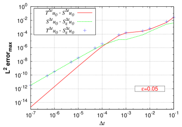
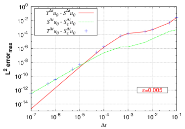
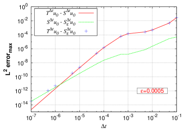
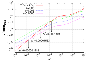
Figure 3: BZ equation. Maximum local $L^{2}$ errors for several splitting time steps $\Delta t$ and $\varepsilon=0.05$ (top left), $0.005$ (top right) and $0.0005$ (bottom left). Bottom right: critical splitting time steps $\Delta t^{\star}$ obtained when $\|T^{\Delta t}u_{0}-S^{\Delta t}u_{0}\|_{L^{2}}\approx\|S^{\Delta t}u_{0}-S^{\Delta t}_{\varepsilon}u_{0}\|_{L^{2}}$ in the numerical tests.

Let us now define the two sets $(a_{1},b_{1},c_{1})$ and $(a_{2},b_{2},c_{2})$, and compute local estimators $e_{1}$ and $e_{2}$ in order to obtain $C_{0}$ according to (40) with $\Delta t=\Delta t_{0}=10^{-5}$; that is a time step for which there is no order loss yet, as seen in Figure 3. As it was previously detailed, we consider $a_{1}=1$ and $a_{2}=c_{1}$ to avoid some extra computations. Furthermore, $b_{2}$ should be close to $b_{1}$, and $c_{1}$ and $c_{2}$ small enough. Setting $b_{1}$ larger than $1/2$ would yield more different $b_{2}$ since $c_{1}=a_{2}$. On the other hand, for $b_{1}$ smaller than $1/2$ we can even set $b_{2}=b_{1}$ but in this case $c_{1}$ will be larger than $1/2$. Therefore, we reach a compromise by setting $b_{1}=1/2$ that yields $c_{1}=a_{2}=1/2$, so we can choose for instance $b_{2}=2/5$ close to $b_{1}$, and thus, $c_{2}=1/10$.

With the local error estimate, $err=\|S^{\Delta t}u_{0}-S^{\Delta t}_{\varepsilon}u_{0}\|_{L^{2}}$, for the various time steps and several $\varepsilon$ shown in Figure 3, Figure 4 presents the estimated critical $\Delta t^{\star}$ calculated with (34) from the estimated $C_{0}(\Delta t_{0})$ and $err$. These critical time steps, $\Delta t^{\star}$, estimated with (34) are in good agreement with numerically measured $\Delta t^{\star}$ in Figure 3, and depend on the value of $\varepsilon$. Hence, the domain of application or working region of the method, $\Delta t\leq\Delta t^{\star}$, might be settled depending on the desired level of accuracy by means of an appropriate choice of $\varepsilon$. For instance, if we consider the case $\varepsilon=0.05$ in Figure 3, for $\Delta t=10^{-6}$, the local error estimate is given by $err\approx 10^{-10}$ whereas the real Strang local error is $\sim 10^{-12}$. This overestimation of the local error will certainly imply an underestimation in the required size of the time steps for a given tolerance. Therefore, for a given tolerance $\eta$ a more suitable configuration should consider an $\varepsilon$ such that $\Delta t\approx\Delta t^{\star}$ in order to reduce excessive overestimations of local errors.

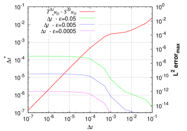
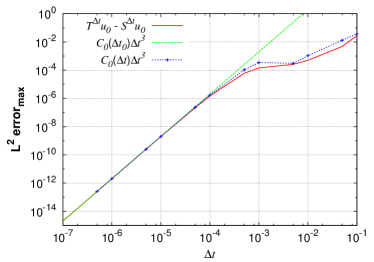
Figure 4: BZ equation. Working region of the method $\Delta t\leq\Delta t^{\star}$ with $\Delta t^{\star}$ calculated with $C_{0}$ estimated at $\Delta t_{0}=10^{-5}$ and $err$ obtained for several splitting time steps $\Delta t$ and $\varepsilon$ (left). Right: predicted Strang error calculated with $C_{0}$ estimated at $\Delta t_{0}=10^{-5}$ and locally at several splitting time steps $\Delta t$.

In the illustration shown in Figure 4, $C_{0}$ was estimated in the third order region of the method and therefore, all values are well approximated as long as $\Delta t$ remains in this region. In particular, critical $\Delta t^{\star}$ will be progressively underestimated for larger $\varepsilon$ and consequently, it will impose smaller time steps for a given tolerance; this is already the case for $\varepsilon=0.05$, for which $\Delta t^{\star}$ is in the transition zone towards the lower order region. Even though the computation of $C_{0}$ with small time steps will be less expensive, a much more accurate procedure considers current time step as shown in Figure 4. In particular, by estimating locally $C_{0}$, we are estimating real Strang error and thus, $\Delta t\leq\Delta t^{\star}$ guarantees prescribed accuracy even if asymptotic order estimates are no longer verified. This allows to properly extend the domain of application over the whole range of possible time steps for a given accuracy; an extremely important issue for real applications for which splitting time steps may go far beyond asymptotic behavior including the potential order reduction region associated with the stiffness of the problem.

5.3 Numerical strategy

Previous studies conducted in $\S~{}$5.1 and $\S~{}$5.2 allow to properly complete the adaptive splitting strategy introduced in $\S~{}$2. In this part we conduct the final description of the numerical strategy.

Let us consider general problem (1) for $\mathbf{u}\in\mathbb{R}^{m}$, for which we use $S_{2}^{t}$ in (6) as resolution scheme. Depending on the problem, the adaptive method will be applied considering time evolution of $l\leq m$ variables: $\mathbf{\tilde{u}}\in\mathbb{R}^{l}$. Let us denote $\Omega_{l}$ the set of indices of these variables. In order to consider only $l<m$ variables, the formers must be decoupled of the remaining $m-l$ variables in the reactive term $\mathbf{f}(\mathbf{\tilde{u}})$ in (1). To simplify the presentation, we will only consider $\varepsilon\in(0,\varepsilon_{max})$, $\varepsilon_{max}<1/2$.

We set the accuracy tolerance $\eta$, an initial time step $\Delta t^{0}$ and initial $\varepsilon_{0}$, and perform the time integration of (1) with the Strang scheme $S_{2}^{t}$ and the embedded shifted one $S^{t}_{2,\varepsilon}$ given by (7). We compute local error estimate $err$ and new time step $\Delta t^{\rm new}$ according to (11). If $err$ is smaller than $\eta$, current time step solution is accepted and simulation time evolves; otherwise, current solution is rejected and the time integration is recomputed with $\Delta t^{\rm new}$. In particular, it is better to choose rather small $\Delta t^{0}$ to avoid initial rejections.

In order to guarantee an effective error control, we define the working region $\Delta t\leq\Delta t^{\star}$ by estimating the corresponding $\Delta t^{\star}$ for current $\varepsilon$. This is done for the first time step $\Delta t^{0}$ and then periodically after $N$ accepted time steps depending on the problem, based on the numerical procedure introduced in $\S~{}$5.1. Computation of critical $\Delta t^{\star}$ is also performed with $\mathbf{\tilde{u}}$, and a rather large initial $\varepsilon_{0}$ is suitable to initially guarantee $\Delta t\leq\Delta t^{\star}$.

We define then a suitable working region $\Delta t\in[\beta\Delta t^{\star},\gamma\Delta t^{\star}]$ with $0<\beta<\gamma\leq 1$, for which splitting time steps are close to $\Delta t^{\star}$. A new $\varepsilon$ is then computed if $\Delta t$ is much lower than $\Delta t^{\star}$ ($\Delta t<\beta\Delta t^{\star}$) in order to avoid unnecessary small time steps; or if $\Delta t$ is very close or possibly larger than $\Delta t^{\star}$ ($\Delta t>\gamma\Delta t^{\star}$) with $\gamma$ close to one, in order to increase upper bound of the domain of application. This guarantees that $\varepsilon$ is dynamically computed and properly adapted to the dynamics of the phenomenon.

Finally, the numerical resolution strategy can be summarized as follows, where $\mathbf{U}\in\mathbb{R}^{m\times n}$ stands for the spatial discretization of $\mathbf{u}$ over $n$ points, $\mathbf{U}:=(u^{(j,k)})$ such that $j\in[1,m]$ and $k\in[1,n]$.

• Input parameters. Define accuracy tolerance $\eta$, time domain of study $[t_{0},T]$, initial time step $\Delta t^{0}$, initial $\varepsilon_{0}$, and period of computation of $\Delta t^{\star}$: $N$.

• Initialization. Set iteration counter $i=0$ and $t=t_{0}$, $\mathbf{U}=\mathbf{U_{0}}$, $\Delta t=\Delta t^{0}$, $\varepsilon=\varepsilon_{0}$. We define a flag $estimate$ initialized as .false.. Throughout the whole computation, we need to store $\mathbf{U}$, an array of size $m\times n$.

• Time evolution. If $t<T$:

  1. Only if $\displaystyle\frac{i}{N}=\left\lfloor\frac{i}{N}\right\rfloor$ or $estimate$ is .true.:
     Computation of critical $\Delta t^{\star}$ I: For the sets $(a_{1},b_{1},c_{1})$ and $(a_{2},b_{2},c_{2})$ with $a_{1}=1$ and $a_{2}=c_{1}$, we compute successively:

     • $\mathbf{\tilde{U}_{1}}=S^{c_{2}\Delta t}\mathbf{\tilde{U}_{0}}$, where $\mathbf{\tilde{U}_{0}}$ is built out of $\mathbf{U}$, $\mathbf{\tilde{U}_{0}}=(u^{(j,\cdot)})_{j\in\Omega_{l}}$;

     • $\mathbf{\tilde{U}_{1}}=S^{b_{2}\Delta t}\mathbf{\tilde{U}_{1}}$;

     • $\mathbf{\tilde{U}_{2}}=S^{c_{1}\Delta t}\mathbf{\tilde{U}_{0}}$;

     • $e_{1}=\max_{j\in\Omega_{l}}\|\tilde{u}_{2}^{(j,\cdot)}-\tilde{u}_{1}^{(j,\cdot)}\|$;

     • $\mathbf{\tilde{U}_{2}}=S^{b_{1}\Delta t}\mathbf{\tilde{U}_{2}}$;

     • $estimate$ is set to .true..

     These operations needs to store $\mathbf{\tilde{U}_{1}}$ and $\mathbf{\tilde{U}_{2}}$, two arrays of size $l\times n$.

  2. Time integration over $\Delta t$: We compute successively:

     • for each $k\in[1,n]$, $u_{new}^{(\cdot,k)}=Y^{\Delta t/2}u^{(\cdot,k)}$;

     • for each $k\in[1,n]$, $\tilde{u}_{1}^{(\cdot,k)}=Y^{\varepsilon\Delta t}\left.u_{new}^{(j,k)}\right|_{j\in\Omega_{l}}$;

     • $\mathbf{U_{\star}}=X^{\Delta t}\mathbf{U_{\star}}$, with $\mathbf{U_{\star}}=\phantom{x}^{t}(\mathbf{U_{new}},\mathbf{\tilde{U}_{1}})$;

     • for each $k\in[1,n]$, $u^{(\cdot,k)}_{\star}=Y^{(1/2-\varepsilon)\Delta t}u^{(\cdot,k)}_{\star}$;

     • for each $k\in[1,n]$, $u^{(\cdot,k)}_{new}=Y^{\varepsilon\Delta t}u^{(\cdot,k)}_{new}$;

     • $err=\max_{j\in\Omega_{l}}\|\tilde{u}_{new}^{(j,\cdot)}-\tilde{u}_{1}^{(j,\cdot)}\|$.

     We need to store $\mathbf{U_{new}}$, an array of size $m\times n$.

  3. Only if $estimate$ is .true.:
     Computation of critical $\Delta t^{\star}$ II: We compute successively:

     • $e_{2}=\max_{j\in\Omega_{l}}\|\tilde{u}_{new}^{(j,\cdot)}-\tilde{u}_{2}^{(j,\cdot)}\|$;

     • $C_{0}$ using (40) with $e_{1}$ and $e_{2}$;

     • estimate $\Delta t^{\star}$ out of (34) and set $\Delta t^{\star}=\zeta\Delta t^{\star}$ with security factor $0<\zeta\leq 1$ close to one;

     • $estimate$ is set to .false..

     • If $\Delta t\notin[\beta\Delta t^{\star},\gamma\Delta t^{\star}]$ with $0<\beta<\gamma\leq 1$: $estimate$ is set to .true..

  4. Only if $estimate$ is .true. and $i>0$:
     Computation of $\varepsilon$: According to (34) with $err$, $C_{0}$ and $\Delta t^{\star}=\Delta t$:

     • $\varepsilon=\min\{\theta\varepsilon,\varepsilon_{max}\}$ with $\theta\geq 1$ as security factor;

     • computation of $\Delta t^{\star}$ with new $\varepsilon$;

     • $estimate$ is set to .false..

  5. Computation $\Delta t^{new}$: According to (11) with security factor $0<\upsilon\leq 1$ close to one.

     • If $\Delta t>\Delta t^{\star}$: set $err=tol+C$ with $C>1$. Used to potentially reject initial $\Delta t=\Delta t^{0}$.

     • If $\Delta t^{new}>\Delta t^{\star}$ and $\varepsilon\neq\varepsilon_{max}$: $estimate$ is set to .true..

     • $\Delta t=\min\{\Delta t^{new},\Delta t^{\star}\}$.

     • If $err\leq tol$: $t=t+\Delta t$, $i=i+1$, $\Delta t=\min\{\Delta t,T-t\}$ and $\mathbf{U}=\mathbf{U_{new}}$.

In this strategy, reaction is always integrated point by point if the reactive term is modeled by a system of ODEs without spatial coupling. This integration can be performed completely in parallel [9, 7]. On the other hand, for linear diffusion problems, another alternative considers a variable by variable resolution, for each $j\in[1,m]\bigcup\Omega_{l}$:

$$u_{\star}^{(j,\cdot)}=X^{\Delta t}u_{\star}^{(j,\cdot)},$$ (42)

that can also be performed in parallel [9].

Depending on the problem, either the computation of critical $\Delta t^{\star}$ (steps (1), (3) and (4)), or the computation of $\varepsilon$ (step (4)) can be potentially removed if one considers large enough $\varepsilon_{0}$ and fine enough $\eta$. Finally, the whole strategy with all steps needs to store at worst two arrays of size $l\times n$ and other two of size $m\times n$, beyond memory requirements of diffusion and reaction solvers.

6 Final Numerical Evaluation of the Method

In this last part, we evaluate the performance of the method in terms of accuracy of the simulation, and show that an effective control of the simulation error is performed in the context of two different problems. First, we will consider a propagating wave featuring time-space multi-scale character. Then, the potential of the method is fully exploited for a more complex configuration of repetitive gas discharges generated by high frequency pulsed applied electric fields followed by long time scale relaxation, for which a precise description of discharge and post-discharge phases is achieved.

6.1 BZ equation revisited

Coming back to BZ model, we perform a time integration of (41) with several accuracy tolerances $\eta$. First of all, we consider the numerical strategy detailed in $\S~{}$5.3 without taking into account steps (1), (3) and (4), that is without computation of neither critical $\Delta t^{\star}$ nor $\varepsilon$. We set $\Delta t^{0}=10^{-7}$ and $\varepsilon_{0}=0.05$ in all cases, with $t\in[0,2]$. In this example, a rather small initial splitting time step is chosen to avoid initial rejections even though this initial rejection phase usually does not take many steps as it will shown in the next example. On the other hand, we have chosen a intermediary value for $\varepsilon$ in order to clearly distinguish the different behaviors of the strategy in terms of prediction of the local errors depending on the proposed tolerance.

Figure 5 shows time evolution of accepted splitting time steps $\Delta t$. In this case, BZ equation models a propagating self-similar wave, so splitting time step stabilizes once the overall phenomenon is solved within the prescribed tolerance $\eta$. Local error estimates $err$ are also shown, which naturally verify prescribed accuracy, since we impose time steps for which $err$ is limited by $\eta$ through (11).

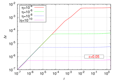
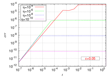
Figure 5: BZ equation. Time evolution of accepted splitting time steps $\Delta t$ (left) and local $L^{2}$ error estimates $err=\|S^{\Delta t}u_{0}-S^{\Delta t}_{\varepsilon}u_{0}\|_{L^{2}}$ (right), for several tolerances $\eta$ and $\varepsilon=0.05$.

Table 2 summarizes global $L^{2}$ errors between splitting and reference solutions at the end of the time domain of study, $t=2$. For a fine enough $\eta$ and consequently, small enough time steps, a precise error control is achieved by the local error control strategy as we could have expected from previous results in Figure 3 for $\varepsilon=0.05$. Nevertheless, for $\eta=10^{-4}$ we can see rather high global errors even if this configuration considers naturally less time integration steps and thus, less accumulation of local approximation errors. If we take a look at Figure 3, we note that for $\varepsilon=0.05$ and local errors of about $10^{-4}$, the local error estimate, $err$, is not predicting properly real Strang errors, as it was previously discussed, since $\Delta t>\Delta t^{\star}$. Therefore, a strategy that introduces a more precise description of errors for a larger range of time steps must be considered, whenever the required accuracy casts the method away from its asymptotic behavior. This is an under covered difficulty of any time adaptive technique based on a lower order embedded method, and to our knowledge, an open problem that has not been studied much, and that this work tries to overcome.

Table 2: BZ equation. $L^{2}$ errors at final time $t=2$ for $a$, $b$, $c$ variables and several tolerances $\eta$.

$\eta$	$L^{2}$ error $a$	$L^{2}$ error $b$	$L^{2}$ error $c$
$10^{-4}$	$7.97\times 10^{-3}$	$1.07\times 10^{-2}$	$4.72\times 10^{-3}$
$10^{-6}$	$1.71\times 10^{-6}$	$1.83\times 10^{-6}$	$7.98\times 10^{-7}$
$10^{-8}$	$1.45\times 10^{-8}$	$1.54\times 10^{-8}$	$6.78\times 10^{-9}$
$10^{-10}$	$1.74\times 10^{-10}$	$1.75\times 10^{-10}$	$1.08\times 10^{-10}$

Let us now consider the entire strategy with all steps for several tolerances with $\Delta t^{0}=5\times 10^{-7}$ and $\varepsilon_{0}=0.05$. In the following illustrations we have considered the following parameters: $\varepsilon_{max}=0.999$; $a_{1}=1$, $b_{1}=c_{1}=a_{2}=1/2$, $b_{2}=2/5$ and $c_{2}=1/10$ for intermediary time steps evaluations; $\zeta=0.9$ as security factor of critical $\Delta t^{\star}$ estimate; $\beta=0.1$ and $\gamma=0.95$ to define the working region $\Delta t\in[\beta\Delta t^{\star},\gamma\Delta t^{\star}]$; $\theta=10$ as security factor of $\varepsilon$ estimate; $C=10$ to potentially reject initial time step $\Delta t^{0}$; and $\upsilon=0.9$ as security factor of $\Delta t^{new}$ estimate. All local estimators, $err$, $e_{1}$ and $e_{2}$, are computed with normalized $L^{2}$ norms.

Considering the propagating phenomenon, we set $N=10$, but we estimate $\Delta t^{\star}$ only twice for $i=0$ and $i=N$. Figure 6 shows time evolution of splitting time steps; there are different scenarios depending on the required accuracy. In all cases for $\varepsilon_{0}=0.05$, we estimate initially $\Delta t^{\star}\approx 1.4\times 10^{-4}$. For $\eta=10^{-4}$, this limitation implies smaller time steps than what is required for the prescribed tolerance. Thus, $\Delta t$ increases until $\Delta t^{new}>\Delta t^{\star}$ and a new $\varepsilon$ is estimated: $\varepsilon\approx 0.43$. No substantial changes are made when $i=N$, since $\Delta t\in[\beta\Delta t^{\star},\gamma\Delta t^{\star}]$ for the current $\eta$.

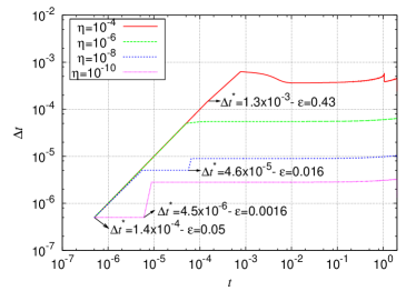
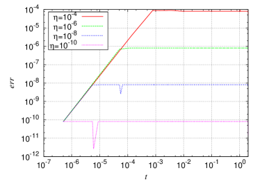
Figure 6: BZ equation. Time evolution of accepted splitting time steps $\Delta t$ (left) and local $L^{2}$ error estimates $err=\|S^{\Delta t}u_{0}-S^{\Delta t}_{\varepsilon}u_{0}\|_{L^{2}}$ (right), for several tolerances $\eta$, considering critical $\Delta t^{\star}$ and computation of $\varepsilon$.

For $\eta=10^{-6}$, we keep initial $\Delta t^{\star}$ and $\varepsilon_{0}$ since $\Delta t\in[\beta\Delta t^{\star},\gamma\Delta t^{\star}]$ as we can see in Figure 3. Finally, for $\eta=10^{-8}$ and $\eta=10^{-10}$, $\Delta t<\beta\Delta t^{\star}$ and thus, $\varepsilon$ is recomputed, giving respectively $\varepsilon\approx 0.016$ and $0.0016$. In particular, we consider larger splitting time steps for which Strang local errors are better predicted. Table 3 shows that error control is this time guaranteed for all values of tolerance $\eta$, and thus, for a larger range of time steps. Compared with previous results in Table 2, we correct completely the errors in the prediction of local error estimates, which yields more accurate resolutions for the largest tolerances; whereas slightly less accurate results are obtained for the smallest tolerances since larger splitting time steps are considered.

Table 3: BZ equation. $L^{2}$ errors at final time $t=2$ for $a$, $b$, $c$ variables and several tolerances $\eta$, considering critical $\Delta t^{\star}$ and computation of $\varepsilon$.

$\eta$	$L^{2}$ error $a$	$L^{2}$ error $b$	$L^{2}$ error $c$
$10^{-4}$	$6.85\times 10^{-5}$	$9.04\times 10^{-5}$	$4.06\times 10^{-5}$
$10^{-6}$	$1.71\times 10^{-6}$	$1.83\times 10^{-6}$	$7.98\times 10^{-7}$
$10^{-8}$	$4.53\times 10^{-8}$	$4.84\times 10^{-8}$	$2.12\times 10^{-8}$
$10^{-10}$	$4.48\times 10^{-9}$	$4.77\times 10^{-9}$	$2.15\times 10^{-9}$

6.2 Simulation of multi-pulsed gas discharges

In this section, we consider a simplified model of plasma discharges at atmospheric pressure for which we analyze the performance of the proposed numerical strategy in a configuration of nanosecond repetitively pulsed discharges. This kind of phenomenon is studied for plasma assisted combustion or flow control, for which the enhancement of the gas flow chemistry or momentum transfer during typical time scales of the flow of $10^{-4}-10^{-3}$s, is due to consecutive discharges generated by high frequency (in the kHz range) sinusoidal or pulsed applied voltages [23]. As a consequence, during the post-discharge phases of the order of tens of microseconds, not only time scales are very different from those during discharges of a few tens of nanoseconds, but a complete different physics is taking place. Then, to the rapid multi-scale configuration during discharges, we have to add other rather slower multi-scale phenomena in the post-discharge, such as recombination of charged species, heavy-species chemistry, diffusion, gas heating and convection. Therefore, it is very challenging to efficiently simulate this kind of highly multi-scale problems and to accurately describe the physics of the plasma/flow interaction between consecutive discharge/post-discharge phases.

General model to study gas discharge dynamics is based on the following drift-diffusion equations for electrons and ions, coupled with Poisson’s equation [2, 20]:

$$\left.\begin{array}[]{rcl}\partial_{t}n_{\rm e}-\partial_{\mathbf{x}}\cdot n_{\rm e}\,\mathbf{v}_{\!\rm e}-\partial_{\mathbf{x}}\cdot(D_{\rm e}\ \partial_{\mathbf{x}}n_{\rm e})&=&n_{\rm e}\alpha|\mathbf{v}_{\rm e}|-n_{\rm e}\eta|\mathbf{v}_{\rm e}|+n_{\rm e}n_{\rm p}\beta_{\rm ep}+n_{\rm n}\gamma,\\ \partial_{t}n_{\rm p}+\partial_{\mathbf{x}}\cdot n_{\rm p}\mathbf{v}_{\!\rm p}-\partial_{\mathbf{x}}\cdot(D_{\rm p}\,\partial_{\mathbf{x}}n_{\rm p})&=&n_{\rm e}\alpha|\mathbf{v}_{\rm e}|-n_{\rm e}n_{\rm p}\beta_{\rm ep}+n_{\rm n}n_{\rm p}\beta_{\rm np},\\ \partial_{t}n_{\rm n}-\partial_{\mathbf{x}}\cdot n_{\rm n}\mathbf{v}_{\!\rm n}-\partial_{\mathbf{x}}\cdot(D_{\rm n}\,\partial_{\mathbf{x}}n_{\rm n})&=&n_{\rm e}\eta|\mathbf{v}_{\rm e}|-n_{\rm n}n_{\rm p}\beta_{\rm np}-n_{\rm n}\gamma,\end{array}\right\}$$ (43)

$$\varepsilon_{0}\,\partial_{\mathbf{x}}^{2}V=-q_{\rm e}(n_{\rm p}-n_{\rm n}-n_{\rm e}),$$ (44)

where $\mathbf{x}\in\mathbb{R}^{d}$, $n_{i}$ is the density of species $i$ (e: electrons, p: positive ions, n: negative ions), $V$ is the electric potential, $\mathbf{v}_{i}=\mu_{i}\mathbf{E}$ ($\mathbf{E}$ being the electric field) is the drift velocity. $D_{i}$ and $\mu_{i}$, are diffusion coefficient and absolute value of mobility of charged species $i$, $q_{\rm e}$ is the absolute value of electron charge, and $\varepsilon_{0}$ is permittivity of free space. $\alpha$ is the impact ionization coefficient, $\eta$ stands for electron attachment on neutral molecules, $\beta_{\rm ep}$ and $\beta_{\rm np}$ accounts respectively for electron-positive ion and negative-positive ion recombination, and $\gamma$ is the detachment coefficient. Electric field $\mathbf{E}$ and potential $V$ are related by

$$\mathbf{E}=-\partial_{\mathbf{x}}V.$$ (45)

Nevertheless, in this paper, we will consider a simplified reaction-diffusion 1D model based on (43):

$$\left.\begin{array}[]{rcl}\partial_{t}n_{\rm e}-D\,\partial^{2}_{x}n_{\rm e}&=&n_{\rm e}\alpha|\mathbf{v}_{\rm e}|-n_{\rm e}\eta|\mathbf{v}_{\rm e}|+n_{\rm e}n_{\rm p}\beta_{\rm ep},\\ \partial_{t}n_{\rm p}-D\,\partial^{2}_{x}n_{\rm p}&=&n_{\rm e}\alpha|\mathbf{v}_{\rm e}|-n_{\rm e}n_{\rm p}\beta_{\rm ep}+n_{\rm n}n_{\rm p}\beta_{\rm np},\\ \partial_{t}n_{\rm n}-D\,\partial^{2}_{x}n_{\rm n}&=&n_{\rm e}\eta|\mathbf{v}_{\rm e}|-n_{\rm n}n_{\rm p}\beta_{\rm np}.\end{array}\right\}$$ (46)

As in (43), all the coefficients of the model are functions of the local reduced electric field $E/N_{\rm gas}$, where $E$ is the electric field magnitude and $N_{\rm gas}$ is the air neutral density. Transport parameters and reaction rates for air are taken from [21], with attachment coefficients taken from [19].

In this numerical illustration, we consider an air gap of $0.5\,$cm where we have a high initial distribution of electrons and ions over the region $[0,0.01]\,$cm. A constant electric field of $\sim 40\,$kV/cm is then applied over this region during $10\,$ns with a pulse period of $1\,\mu$s. All parameters in (46) are computed with the imposed field without solving neither (44) nor (45). Finally, we consider a constant diffusion coefficient: $D=50\,$cm²/s and a spatial discretization of $1001$ points. Figure 7 shows the spatial distribution of electron density just before and after each pulse. Globally, there are at least two completely different physical configurations given either by high reactive activity whenever the electric field is applied, or rather by the propagative nature of the post-discharge phase.

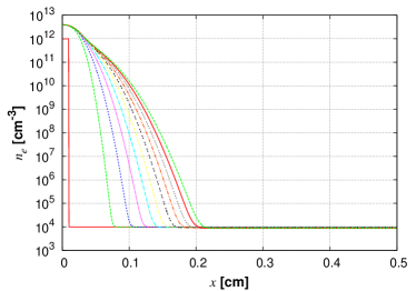
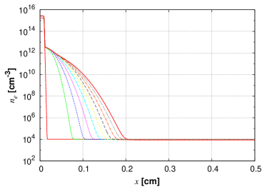
Figure 7: Repetitive gas discharge model. Spatial distribution of electron density before (left) and after (right) each pulse, starting from initial distribution (left) and for a duration of ten pulses.

Considering the adaptive strategy described in $\S~{}$5.3 with $\Delta t^{0}=10^{-10}$, $\varepsilon_{0}=0.05$ and the same parameters used for the previous BZ simulation, computation is initialized with a time step included in the pulse duration. Figure 8 shows the corresponding splitting time steps for a tolerance of $\eta=10^{-3}$. Splitting time step features a periodic behavior and succeed to consistently adapt itself to the discharge/post-discharge phenomena. This yields high varying time steps going from $\sim 10^{-10}$ to $\sim 10^{-7}$. Therefore, after each post-discharge phase, since the new time step is computed based on the previous one according to (11), this new time step will surely skip the next pulse. In order to avoid this, each time we get into a new period, we initialize time step with the length of the pulse: $\Delta t=10\,$ns; this time step is obviously rejected as seen in Figure 8, as well as the next ones, until we are able to retrieve the right dynamics of the phenomenon for the required accuracy tolerance. No other intervention is needed neither for modeling parameters nor for numerical solvers in order to automatically adapt time step to describe the several time scales of the phenomenon within a prescribed accuracy.

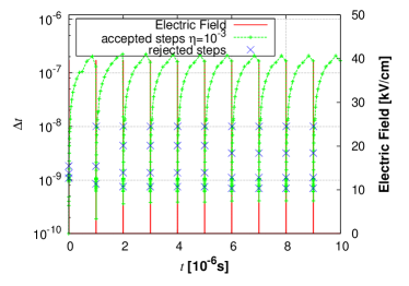
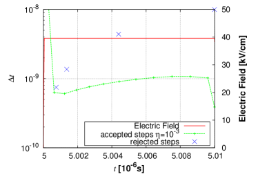
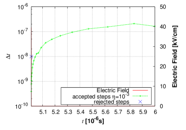
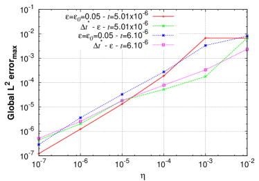
Figure 8: Repetitive gas discharge model. Time evolution of accepted and rejected splitting time steps, and imposed electric field for $t\in[0,10]\,\mu$s (top left), during pulse $t\in[5,5.01]\,\mu$s (top right) and post-discharge $t\in[5.01,6]\,\mu$s (bottom left). Bottom right: global $L^{2}$ errors at the end of the pulse ($t=5.01\,\mu$s) and the post-discharge phase ($t=6\,\mu$s) with and without $\Delta t^{\star}$ and $\varepsilon$ computation.

For this application, we compute critical $\Delta t^{\star}$ and possibly $\varepsilon$, for $N=10$ and $N=100$ in each period in order to perform these computations at least once during the discharge and post-discharge regimes. For example, for $t\in[5,6]\,\mu$s as in Figure 8, $\varepsilon=\varepsilon_{max}$ with $\Delta t^{\star}\approx 4.3\times 10^{-9}$ during the pulse, and $\varepsilon\approx 0.26$ with $\Delta t^{\star}\approx 1.6\times 10^{-7}$ for the rest of the period. Similar values are found for the other periods. Notice that after each pulse, $\Delta t^{\star}$ is automatically updated because $\Delta t$ increases and then $\Delta t$ gets equal to $\Delta t^{\star}$. In particular, the important difference between $\Delta t^{\star}$ for each region, comes naturally from the completely different modeling parameters and hence, physics description of each regime.

An effective error control is achieved for each part of the phenomenon, as we can deduce from the global error between splitting and reference solutions at the end of the pulse ($t=5.01\,\mu$s) and at the end of the post-discharge phase ($t=6\,\mu$s). If we compare these results with the ones obtained without estimating neither $\Delta t^{\star}$ nor $\varepsilon$ with $\varepsilon=\varepsilon_{0}=0.05$, we can draw the same conclusions as in the BZ application. For less accurate resolutions with high tolerances, the proposed strategy corrects the error in the local error estimates made with $\varepsilon=\varepsilon_{0}=0.05$; in particular, for $\eta=10^{-3}$ there is a ratio of about $10$ between both solutions. For higher tolerances, $\eta\geq 10^{-2}$, both methods yield a time step equal to the pulse duration, $\Delta t=10\,$ns. On the other hand, for the smallest tolerances, slightly more accurate solutions are obtained with a fixed $\varepsilon=\varepsilon_{0}$ because smaller splitting time steps are used.

7 Conclusions

The present work proposes a new resolution strategy for stiff evolutionary PDEs based on an efficient splitting scheme previously developed [9, 8] that considers high order dedicated integration methods for each subproblem in order to properly solve the fastest time scales associated with each one of them, and in such a way that the main source of error is led by the operator splitting error. Then, to control the error of the resolution, it relies on an adaptive splitting time technique that allows to discriminate the global time scales related to the coupled phenomenon, given a required level of accuracy of computations. Compared with a standard procedure for which accuracy is guaranteed by considering time steps of the order of the fastest scale, the error control featured by our method implies an effective accurate resolution for problems modeling various physical scenarios, independent of the fastest physical time scale, and an important improvement of computational efficiency whenever highly unsteady phenomena is simulated. In particular, we have successfully applied the proposed strategy to a simplified model of plasma discharges that nevertheless exhibits a broad time scale spectrum coming from the modeling equations and also important and discontinuous variation of parameters in time and in space that notably increase the numerical complexity of the problem.

A numerical analysis of the method has been developed in order to settle a solid mathematical background, and a complementary numerical procedure was conceived in order to overcome classical restrictions of adaptive time stepping schemes whenever asymptotic estimates fail to predict the dynamics of the problem. A both mathematical and numerical detailed study of the method has thus led to a fully complete adaptive time stepping strategy that guarantees an effective control of the errors of integration for a large range of time steps; a key issue for problems for which splitting time steps can go beyond the fastest physical scales of the problem. The contribution of this paper is then mainly given by a dedicated adaptive time splitting method for stiff PDEs, and by a complete study of the behavior of time stepping schemes based on lower order embedded methods, for the whole set of potential time steps. In this paper we have always considered fine enough spatial discretizations in order to perform an evaluation of the theoretical estimates introduced for the proposed time integration scheme. For higher dimensional problems, fine spatial discretization becomes a critical issue in terms of computational costs and a technique of local grid refinement might be a good solution to guarantee the theoretical behavior of the splitting schemes (see for instance [8]). Nevertheless, a mathematical study on the splitting errors with discretized operators will certainly be an useful tool to yet improve the performance of these techniques. This and other related theoretical aspects are particular topics of our current research.

References

- [1] A. Abdulle. Fourth order Chebyshev methods with recurrence relation. SIAM J. Sci. Comput., 23:2041–2054, 2002.
- [2] N. Y. Babaeva and G. V. Naidis. Two-dimensional modelling of positive streamer dynamics in non-uniform electric fields in air. J. Phys. D: Appl. Phys., 29:2423–2431, 1996.
- [3] S. Descombes, T. Dumont, V. Louvet, and M. Massot. On the local and global errors of splitting approximations of reaction-diffusion equations with high spatial gradients. Int. J. of Computer Mathematics, 84(6):749–765, 2007.
- [4] S. Descombes, T. Dumont, and M. Massot. Operator splitting for stiff nonlinear reaction-diffusion systems: Order reduction and application to spiral waves. In Patterns and waves (Saint Petersburg, 2002), pages 386–482. AkademPrint, St. Petersburg, 2003.
- [5] S. Descombes and M. Massot. Operator splitting for nonlinear reaction-diffusion systems with an entropic structure: Singular perturbation and order reduction. Numer. Math., 97(4):667–698, 2004.
- [6] S. Descombes and M. Thalhammer. The Lie-Trotter splitting method for nonlinear evolutionary problems involving critical parameters. An exact local error representation and application to nonlinear Schrödinger equations in the semi-classical regime. Preprint, available on HAL (http://hal.archives-ouvertes.fr/hal-00557593), 2010.
- [7] M. Duarte, M. Massot, S. Descombes, C. Tenaud, T. Dumont, V. Louvet, and F. Laurent. New resolution strategy for multi-scale reaction waves using time operator splitting and space adaptive multiresolution: Application to human ischemic stroke. ESAIM Proc. (to app.), 2011.
- [8] M. Duarte, M. Massot, S. Descombes, C. Tenaud, T. Dumont, V. Louvet, and F. Laurent. New resolution strategy for multi-scale reaction waves using time operator splitting, space adaptive multiresolution and dedicated high order implicit/explicit time integrators. Submitted to SIAM J. Sci. Comput., available on HAL (http://hal.archives-ouvertes.fr/hal-00457731), 2011.
- [9] T. Dumont, M. Duarte, S. Descombes, M.A. Dronne, M. Massot, and V. Louvet. Simulation of human ischemic stroke in realistic 3D geometry: A numerical strategy. Submitted to Bulletin of Math. Biology, available on HAL (http://hal.archives-ouvertes.fr/hal-00546223), 2011.
- [10] I. R. Epstein and J. A. Pojman. An Introduction to Nonlinear Chemical Dynamics. Oxford University Press, 1998. Oscillations, Waves, Patterns and Chaos.
- [11] P. Gray and S. K. Scott. Chemical oscillations and instabilites. Oxford University Press, 1994.
- [12] W. Gröbner. Die Liereihen und ihre Anwendungen. VEB Deutscher Verlag der Wiss., Berlin 1960, 1967. Second Edition.
- [13] E. Hairer, C. Lubich, and G. Wanner. Geometric Numerical Integration. Springer-Verlag, Berlin, second edition, 2006. Structure-Preserving Algorithms for Odinary Differential Equations.
- [14] E. Hairer, S. P. Nørsett, and G. Wanner. Solving ordinary differential equations I. Springer-Verlag, Berlin, second edition, 1993. Nonstiff problems.
- [15] E. Hairer and G. Wanner. Solving ordinary differential equations II. Springer-Verlag, Berlin, second edition, 1996. Stiff and differential-algebraic problems.
- [16] O. M. Knio, H. N. Najm, and P. S. Wyckoff. A semi-implicit numerical scheme for reacting flow. II. Stiff, operator-split formulation. J. Comput. Phys., 154:482–467, 1999.
- [17] O. Koch and M. Thalhammer. Embedded split-step formulae for the time integration of nonlinear evolution equations. Preprint, 2010.
- [18] A. N. Kolmogoroff, I. G. Petrovsky, and N. S. Piscounoff. Etude de l’équation de la diffusion avec croissance de la quantité de matière et son application a un problème biologique. Bulletin de l’Université d’état Moscou, Série Internationale Section A Mathématiques et Mécanique, 1:1–25, 1937.
- [19] I. A. Kossyi, A. Yu Kostinsky, A. A. Matveyev, and V. P. Silakov. Kinetic scheme of the non-equilibrium discharge in nitrogen-oxygen mixtures. Plasma Sources Sci. Technol., 1(3):207–220, 1992.
- [20] A. A. Kulikovsky. Positive streamer between parallel plate electrodes in atmospheric pressure air. J. Phys. D: Appl. Phys., 30:441–450, 1997.
- [21] R. Morrow and J. J. Lowke. Streamer propagation in air. J. Phys. D: Appl. Phys., 30:614–627, 1997.
- [22] E. S. Oran and J. P. Boris. Numerical simulation of reacting flows. Cambridge University Press, 2001. Second Edition.
- [23] G. Pilla, D. Galley, D. Lacoste, F. Lacas, D. Veynante, and C. O. Laux. Stabilization of a turbulent premixed flame using a nanosecond repetitively pulsed plasma. IEEE Trans. Plasma Sci., 34(6, Part 1):2471–2477, 2006.
- [24] M. A. Singer, S. B. Pope, and H. N. Najm. Modeling unsteady reacting flow with operator splitting and ISAT. Combustion and Flame, 147(1-2):150 – 162, 2006.
- [25] G. Strang. Accurate partial difference methods. I. Linear Cauchy problems. Arch. Ration. Mech. Anal., 12:392–402, 1963.
- [26] G. Strang. On the construction and comparison of difference schemes. SIAM J. Numer. Anal., 5:506–517, 1968.