Anisotropic Mobility Model for Polymers under Shear
and its Linear Response Functions

Abstract

We propose a simple dynamic model of polymers under shear with an anisotropic mobility tensor. We calculate the shear viscosity, the rheo-dielectric response function, and the parallel relaxation modulus under shear flow deduced from our model. We utilize recently developed linear response theories for nonequilibrium systems to calculate linear response functions. Our results are qualitatively consistent with experimental results. We show that our anisotropic mobility model can reproduce essential dynamical nature of polymers under shear qualitatively. We compare our model with other models or theories such as the convective constraint release model or nonequilibrium linear response theories.

I Introduction

The linear response theory gives a formula which relates a response function in equilibrium to an equilibrium time correlation function Kubo et al. (1991); Evans and Morris (2008); Risken (1989). In equilibrium, the response of a physical quantity $A$ at time $t$ to a weak external perturbation at time $t^{\prime}(\leq t)$, which is conjugate to $B$, is given as the following form.

$$\mathcal{R}_{AB}(t-t^{\prime})=\frac{1}{k_{B}T}\frac{d}{dt^{\prime}}\langle A(t)B(t^{\prime})\rangle_{\text{eq}}$$ (1)

Here $k_{B}$ is the Boltmzann constant, $T$ is the absolute temperature, and $\langle\dotsb\rangle_{\text{eq}}$ means the equilibrium statistical average. Eq (1) holds for a wide range of systems Kubo et al. (1991); Evans and Morris (2008); Risken (1989) as long as the system is in equilibrium. (In the followings, we call the response formula (1) as the Green-Kubo type formula.) From the view point of experiments, eq (1) can be utilized to obtain the correlation function from the response function. This enables us to extract information of microscopic and/or mesoscopic dynamics of molecules from macroscopic responses.

For polymeric systems, the viscoelastic response functions (especially the shear relaxation modulus or the storage and loss moduli) or the dielectric response function are useful. For example, the viscoelastic response functions can be related to the autocorrelation function of the microscopic stress tensor, and the stress tensor can be related to bond vectors Doi and Edwards (1986). The dielectric response functions of polymers with type A dipoles (polymer chains which have electric dipoles along the chain backbones) can be related to the autocorrelation functions of end-to-end vectors. The combination of the viscoelastic and dielectric measurements provides various information about dynamics of polymer chains Watanabe (1999); Matsumiya et al. (2000); Watanabe et al. (2000); Matsumiya and Watanabe (2001); Watanabe et al. (2002a).

Even out of equilibrium, it is possible to measure linear response functions. Then we expect that the measured response functions can be related to the correlation functions, or at least they reflect the information about the dynamics of polymer chains. Actually, several linear response measurements under steady shear, such as mechanical responses Osaki et al. (1965); de L. Costello (1997); Vermant et al. (1998); Isayev and Wong (1988); Wong and Isayev (1989); Somma et al. (2007); Boukany and Wang (2009); Li and Wang (2010) or dielectric responses Matsumiya et al. (1998); Watanabe et al. (1999, 2002b, 2003a, 2005) have been reported. However, unlike the equilibrium cases, it is not clear how we can analyze and interpret the nonequilibrium linear response functions. In several works, the Green-Kubo type relation (1) is utilized to analyze obtained experimental data, without justifications. But from the view point of nonequilibrium statistical physics, generally eq (1) does not hold except for some special or limited cases.

Fortunately, the Green-Kubo type relation approximately holds for the dielectric response of polymers in the shear gradient direction under shear (the rheo-dielectric response) Uneyama et al. (2009), and thus we can obtain the correlation function of the end-to-end vectors under shear. In this work we therefore concentrate on polymers with type A dipoles. The rheo-dielectric responses for polymers with type A dipoles has been systematically studied and analyzed for various systems and shear rates Matsumiya et al. (1998); Watanabe et al. (2002b, 2003a, 2005), The rheo-dielectric functions of linear polymers are reported to be insensitive to shear, even if the shear rate is large and the shear thinning is observed. This implies that the dynamics of polymer chains in the shear gradient direction is not affected largely by shear flow even under fast shear. So far, why and how such insensitivity occurs is not fully understood. Although attempts have been done by coarse-grained molecular simulations Masubuchi et al. (2004); Uneyama et al. (2009), simulations have failed to reproduce experimentally obtained rheo-dielectric behavior.

In the field of the constitutive equation models, many different approaches to nonequilibrium systems have been utilized, to reproduce nonlinear viscoelasticity well. Among them, the anisotropic mobility type models Curtiss and Bird (1980a, b); Giesekus (1982); Arsac et al. (1994); Stephanou et al. (2009); Beris and Edwards (1994) are particularly notable. In the anisotropic friction model, the friction coefficient (or almost equivalently, the relaxation time) of the model is expressed as a tensor quantity instead of a scalar quantity. This allows us to reproduce variety of models which can reproduce complex viscoelastic behavior with relatively simple constitutive equations.

Motivated by the anisotropic mobility type constitutive equation models, in this work we aim to propose a Langevin equation model with an anisotropic mobility tensor for dynamics of polymers under shear. Although the anisotropic mobility tensors are not utilized widely in the field of the nonequilibrium statistical mechanics, they can potentially model the dynamics under fast shear. A Langevin equation model with an anisotropic mobility tensor model was already proposed for a rather simple system McPhie et al. (2001) based on the projection operator method and molecular dynamics simulation data. We construct an anisotropic mobility model which is consistent with some molecular dynamics simulation results, in a similar way. We limit ourselves to an analytically solvable toy model to examine the characteristic properties of the anisotropic mobility model explicitly and simply. We explicitly calculate several linear response functions such as the rheo-dielectric response function and the moduli in the shear flow direction (parallel moduli) for our model. To calculate the linear response functions, we utilize recently developed linear response theories for nonequilibrium Langevin systems Baiesi et al. (2009a, b); Seifert and Speck (2001). Finally we discuss the properties of our model and its linear response functions under shear from several aspects. We compare our model with several pieces of previous work, and show the differences and similarities between our model and the other models.

II Model

In this section, we propose a simple and solvable model for dynamics of polymers under shear. We consider weakly entangled polymer melts or solutions, for which rheo-dielectric experiments have been carried out Matsumiya et al. (1998); Watanabe et al. (2002b, 2003a, 2005). There are several different approaches to model the dynamics of polymers Doi and Edwards (1986); Watanabe (1999); McLeish (2002); Kröger (2004). Thus at first, we should choose an appropriate model from candidates. We are interested in the qualitative and essential feature of the polymer dynamics under shear. We require the model to be simple and analytically solvable, so that we avoid unnecessary complexities and confusions, and make the model properties clear. From these requirements, we limit ourselves to the dynamics of the end-to-end vector of a single polymer chain $\bm{R}$, in the weakly entangled system. This reduces the degrees of freedom drastically. (This approximation gives so-called the dumbbell model Kröger (2004).) We also limit ourselves to the dynamics in the long time limit, where is no memory effect for the end-to-end vector dynamics. Then we can describe the dynamic equation for $\bm{R}$ in a closed, Markovian form. In equilibrium, this equation can be described as

$$\frac{d\bm{R}(t)}{dt}=-\frac{1}{\zeta_{0}}\frac{\partial\mathcal{F}(\bm{R}(t))}{\partial\bm{R}(t)}+\bm{\xi}_{0}(t)$$ (2)

where $\zeta_{0}$ is the friction coefficient which the end-to-end vector feels, $\mathcal{F}(\bm{R})$ is the free energy, and $\bm{\xi}_{0}(t)$ is the Gaussian noise. For a Gaussian chain, the free energy can be expressed in the following simple linear elasticity form.

$$\mathcal{F}(\bm{R})=\frac{3k_{B}T}{2\bar{R}^{2}}\bm{R}^{2}$$ (3)

$\bar{R}^{2}$ is the equilibrium mean square average end-to-end distance. The fluctuation-dissipation relation of the second kind Kubo et al. (1991) requires for the thermal noise $\bm{\xi}_{0}(t)$ to satisfy the following relations.

$$\langle\bm{\xi}_{0}(t)\rangle=0$$ (4)

$$\langle\bm{\xi}_{0}(t)\bm{\xi}_{0}(t^{\prime})\rangle=\frac{2k_{B}T}{\zeta_{0}}\delta(t-t^{\prime})\bm{1}$$ (5)

Here $\langle\dotsb\rangle$ denotes the statistical average and $\bm{1}$ is the unit tensor.

We consider a system under simple shear. The velocity gradient tensor $\bm{\kappa}$ is given as follows.

$$\kappa_{\alpha\beta}=\begin{cases}\dot{\gamma}&(\alpha=x,\beta=y)\\ 0&(\text{otherwise})\end{cases}$$ (6)

where $\dot{\gamma}$ is the shear rate. We assume that $\dot{\gamma}$ is smaller than $\tau_{R}^{-1}$ ($\tau_{R}$ is the Rouse time of the polymer chain) and the polymer chain is not so highly stretched. A schematic image of the system is shown in FIG. 1. Since the shear flow cannot be expressed in relation to a conservative potential force, the system is nonequilibrium under simple shear. As a simple extension of the equilibrium Langevin equation (2), one may consider the following Langevin equation.

$$\frac{d\bm{R}(t)}{dt}=-\frac{1}{\zeta_{0}}\frac{\partial\mathcal{F}(\bm{R}(t))}{\partial\bm{R}(t)}+\bm{\kappa}\cdot\bm{R}(t)+\bm{\xi}_{0}(t)$$ (7)

In the Langevin equation (7), the mobility, which is defined as the inverse of the friction coefficient, is scalar and thus isotropic. This is because we simply used the mobility (the friction tensor) in equilibrium. The system is isotropic in equilibrium, and the mobility should also be isotropic from the symmetry. However, if the system is not in or near equilibrium, it is generally not isotropic. This means that, in principle, the mobility could be an anisotropic, tensor quantity McPhie et al. (2001). Actually, in some constitutive equation models Giesekus (1982); Beris and Edwards (1994), the mobility tensors are designed to be anisotropic under flow. Thus we consider that eq (7) is an oversimplified dynamic equation model, which may lead physically incorrect results in particular under fast flow.

When the mobility tensor becomes anisotropic, we expect that some transport coefficient tensors also become anisotropic Sarman et al. (1991); Evans (1991); Evans et al. (1992). Anisotropic diffusion coefficient tensors are actually observed in nonequilibrium molecular dynamics (NEMD) simulations based on the SLLOD model Sarman et al. (1992); Hunt and Todd (2009). The diffusion tensor of Lennard-Jones (LJ) particles under shear is first reported by Sarman, Evans, and Baranyai Sarman et al. (1992). They studied the diffusion tensor of an LJ particle under shear, at various rates. Their simulation result clearly shows that the diffusion tensor becomes anisotropic and it depends on the shear rate. Quite recently, Hunt and Todd Hunt and Todd (2009) performed NEMD simulations for relatively short polymer melts (the Kremer-Grest chains Kremer and Grest (1990)) and measured the diffusion tensors under shear. Their result is qualitatively similar to the case of the LJ system. Namely, the diffusion tensor of the center of mass of a polymer chain becomes anisotropic and depends on the shear rate. Besides, the dependence of the diffusion tensor on the shear rate becomes strong as the polymerization index (number of beads in a chain) increases. Although their simulations are limited for rather short chains (unentangled chains), we expect that this trend will be qualitatively the same or even enhanced for well entangled chains.

Although there are several possible interpretations for these NEMD results Baranyai (2000); McPhie et al. (2001), in this work we interpret that the anisotropic diffusion is caused by anisotropic mobilities. Namely, if we model the dynamics of a polymer chain under shear by a Langevin equation, we should employ an anisotropic mobility tensor (or an anisotropic friction tensor). McPhie et al McPhie et al. (2001) proposed a Langevin equation with an anisotropic friction tensor to describe the coarse-grained motion of an LJ particle under shear. Although they proposed an underdamped Langevin equation, an overdamped Langevin equation (like eq (2)) seems to be more suitable for the end-to-end vector of a polymer. Then we express the Langevin equation under shear as follows.

$$\frac{d\bm{R}(t)}{dt}=-\bm{\Lambda}(\dot{\gamma})\cdot\frac{\partial\mathcal{F}(\bm{R})}{\partial\bm{R}}+\bm{\kappa}\cdot\bm{R}+\bm{\xi}(\dot{\gamma};t)$$ (8)

where $\bm{\Lambda}(\dot{\gamma})$ is the mobility tensor which depends on the shear rate $\dot{\gamma}$ and $\bm{\xi}(\dot{\gamma},t)$ is the Gaussian noise. We assume that the fluctuation-dissipation type relation between $\bm{\xi}(\dot{\gamma},t)$ and $\bm{\Lambda}(\dot{\gamma})$ is satisfied.

$$\langle\bm{\xi}(\dot{\gamma};t)\rangle=0$$ (9)

$$\langle\bm{\xi}(\dot{\gamma};t)\bm{\xi}(\dot{\gamma};t^{\prime})\rangle=2k_{B}T\bm{\Lambda}(\dot{\gamma})\delta(t-t^{\prime})$$ (10)

Eq (10) requires the mobility tensor $\bm{\Lambda}(\dot{\gamma})$ to be symmetric under the shear field given by eq (6). Quite recently, Ilg and Kröger Ilg (2010); Ilg and Kröger (2011) proposed a constitutive equation model with anisotropic mobility (friction coefficient) tensor for relatively short polymer chains, based on the NEMD results. Although their model is not equivalent to ours, it is qualitatively similar.

From NEMD simulation results and properties of a Langevin type equation, we consider the mobility tensor $\bm{\Lambda}(\dot{\gamma})$ under steady shear should have the following properties.

• The mobility tensor should be positive definite (all of its eigenvalues should be positive).

• The eigenvalues of $\bm{\Lambda}(\dot{\gamma})$ are unchanged under the transform $\dot{\gamma}\to-\dot{\gamma}$. That is, each eigenvalue is an even function of $\dot{\gamma}$.

• The $xx$-component ($\Lambda_{xx}$) decreases as $\dot{\gamma}$ increases, while other diagonal components ($\Lambda_{yy}$ and $\Lambda_{zz}$) are not so sensitive to $\dot{\gamma}$.

• The $xy$-component ($\Lambda_{xy}$) is non-zero but its value is smaller than diagonal elements. Thus it may be simply neglected ($\Lambda_{xy}\approx 0$).

• From the symmetry, $\Lambda_{xz}=\Lambda_{yz}=0$.

• The mobility tensor should reduce to the isotropic tensor at equilibrium ($\dot{\gamma}=0$).

In this work, we employ the following simple form which satisfies the above properties. (We discuss about the other possible forms later.)

$$\bm{\Lambda}(\dot{\gamma})=\frac{1}{\zeta_{0}}\begin{bmatrix}\tilde{\lambda}(\dot{\gamma})&0&0\\ 0&1&0\\ 0&0&1\end{bmatrix}$$ (11)

Here, $\zeta_{0}$ is the friction coefficient at equilibrium and $\tilde{\lambda}(\dot{\gamma})$ is a function of $\dot{\gamma}$. $\tilde{\lambda}(\dot{\gamma})$ is an even function of $\dot{\gamma}$, and it monotonically increases as $\dot{\gamma}^{2}$ increases. Further, since it should recover the equilibrium form in the absence of shear flow, $\tilde{\lambda}(\dot{\gamma})$ reduces to the equilibrium form, $\tilde{\lambda}(0)=1$, at the limit of $\dot{\gamma}\to 0$. For example, we can employ the following simple form for $\tilde{\lambda}(\dot{\gamma})$.

$$\tilde{\lambda}(\dot{\gamma})=\left[1+(\tau_{c}\dot{\gamma})^{2}\right]^{\alpha/2}$$ (12)

$\alpha$ is an exponent which satisfies $0\leq\alpha\leq 1$, and $\tau_{c}$ is a characteristic crossover time. Roughly speaking, the mobility tensor is isotropic for $|\tau_{c}\dot{\gamma}|\ll 1$ and anisotropic for $|\tau_{c}\dot{\gamma}|\gg 1$. As we show in the next section, eq (12) gives the power law type behavior of the shear viscosity. We call eq (12) as the power law type model. We can also employ the following form.

$$\tilde{\lambda}(\dot{\gamma})=1+\frac{\zeta_{0}-\zeta_{\infty}}{\zeta_{\infty}}\frac{(\tau_{c}\dot{\gamma})^{2}}{1+(\tau_{c}\dot{\gamma})^{2}}$$ (13)

$\zeta_{\infty}$ corresponds to the effective friction coefficient in the $x$-direction for $|\tau_{c}\dot{\gamma}|\gg 1$. Eq (13) may be preferred if the system exhibits the second Newtonian region for the shear viscosity. Eqs (12) and (13) are just possible candidates, and there are many other possible forms for $\tilde{\lambda}(\dot{\gamma})$. It is worth noting that our anisotropic mobility tensor is qualitatively similar to the model by Ilg and Kröger Ilg (2010); Ilg and Kröger (2011) (in their model, the dynamics of the $x$-direction is also accelerated under shear). Before we proceed, we should notice that the anisotropic mobility tensor (11) is designed for the simple shear flow, and it is not expected to be applicable for other flows such as elongational flows. In the following analysis, we consider the response around the steady state under the simple shear (expressed by eq (6)) and thus eq (11) is sufficient for our purpose.

Since the Langevin equation (8) is linear in $\bm{R}$, we can analytically integrate it and obtain explicit expression for several physical quantities. Thus we can analyze linear responses such as the rheo-dielectric response of our model explicitly. By substituting eq (11) into eq (8), we have the following equations for $R_{x},R_{y},$ and $R_{z}$.

$$\frac{dR_{x}(t)}{dt}=-\frac{\tilde{\lambda}(\dot{\gamma})}{\tau_{0}}R_{x}(t)+\dot{\gamma}R_{y}(t)+\xi_{x}(\dot{\gamma},t)$$ (14)

$$\frac{dR_{y}(t)}{dt}=-\frac{1}{\tau_{0}}R_{y}(t)+\xi_{y}(\dot{\gamma},t)$$ (15)

$$\frac{dR_{z}(t)}{dt}=-\frac{1}{\tau_{0}}R_{z}(t)+\xi_{z}(\dot{\gamma},t)$$ (16)

where we defined the characteristic time $\tau_{0}$.

$$\tau_{0}\equiv\frac{\zeta_{0}\bar{R}^{2}}{3k_{B}T}$$ (17)

The probability distribution defined via the following equation is useful for some calculations.

$$P(\bm{r},t)\equiv\langle\delta(\bm{r}-\bm{R}(t))\rangle$$ (18)

The probability density (18) follows the Fokker-Planck equation, which describes the time evolution due to the Langevin equation (8).

$$\frac{\partial P(\bm{r},t)}{\partial t}=\frac{\partial}{\partial\bm{r}}\cdot\bm{\Lambda}(\dot{\gamma})\cdot\left[\frac{\partial\mathcal{F}(\bm{r})}{\partial\bm{r}}P(\bm{r},t)+k_{B}T\frac{\partial P(\bm{r},t)}{\partial\bm{r}}\right]-\frac{\partial}{\partial\bm{r}}\cdot\left[\bm{\kappa}\cdot\bm{r}P(\bm{r},t)\right]$$ (19)

The steady state solution of the Fokker-Planck equation (19), $P_{\text{ss}}(\bm{r})$ satisfies

$$0=\frac{\partial}{\partial\bm{r}}\cdot\bm{\Lambda}(\dot{\gamma})\cdot\left[\frac{\partial\mathcal{F}(\bm{r})}{\partial\bm{r}}P_{\text{ss}}(\bm{r})+k_{B}T\frac{\partial P_{\text{ss}}(\bm{r})}{\partial\bm{r}}\right]-\frac{\partial}{\partial\bm{r}}\cdot\left[\bm{\kappa}\cdot\bm{r}P_{\text{ss}}(\bm{r})\right]$$ (20)

For a linear Fokker-Planck equation, the steady state probability distribution is known to be a Gaussian Risken (1989). Thus we can describe the explicit form of $P_{\text{ss}}(\bm{r})$ simply as follows.

$$P_{\text{ss}}(\bm{r})=\frac{1}{\sqrt{\det[2\pi\bm{C}(\dot{\gamma})]}}\exp\left[-\frac{1}{2}\bm{r}\cdot\bm{C}^{-1}(\dot{\gamma})\cdot\bm{r}\right]$$ (21)

Here $\bm{C}(\dot{\gamma})$ is the covariance matrix.

$$\bm{C}(\dot{\gamma})\equiv\frac{\bar{R}^{2}}{3}\begin{bmatrix}\displaystyle 1+\frac{(\tau_{0}\dot{\gamma})^{2}}{\tilde{\lambda}(1+\tilde{\lambda})}&\displaystyle\frac{\tau_{0}\dot{\gamma}}{1+\tilde{\lambda}}&0\\ \displaystyle\frac{\tau_{0}\dot{\gamma}}{1+\tilde{\lambda}}&1&0\\ 0&0&1\end{bmatrix}$$ (22)

For any physical quantity determined by $\bm{R}$, the statistical average of a function of $\bm{R}$ in the steady state can be evaluated easily with the aid of the steady state probability distribution (21). Also, we can construct the constitutive equation of the anisotropic mobility model from the Fokker-Planck equation (19). We show the constitutive equation and compare it with some conventional constitutive equation models in Appendix A.

III Results

III.1 Shear Viscosity

In our model, the stress tensor is expressed as follows.

$$\bm{\sigma}(\bm{R})=\frac{3\nu_{0}k_{B}T}{\bar{R}^{2}}\bm{R}\bm{R}$$ (23)

where $\nu_{0}$ is the number density of polymer chains. The steady state statistical average of eq (23) can be evaluated easily by using eqs (21) and (22). The shear viscosity at the steady state is expressed as

$$\eta(\dot{\gamma})\equiv\frac{\langle\sigma_{xy}\rangle_{\text{ss}}}{\dot{\gamma}}$$ (24)

where $\langle\dotsb\rangle_{\text{ss}}$ denotes the statistical average in the steady state (under shear). Finally we have the following expression for the steady state shear viscosity $\eta(\dot{\gamma})$.

$$\eta(\dot{\gamma})=\frac{3\nu_{0}k_{B}T}{\bar{R}^{2}\dot{\gamma}}C_{xx}(\dot{\gamma})=\eta_{0}\frac{2}{1+\tilde{\lambda}}$$ (25)

Here $\eta_{0}$ is the Newtonian viscosity in the limit of $\dot{\gamma}\to 0$, $\eta_{0}\equiv\nu_{0}k_{B}T\tau_{0}/2$. Eq (25) is a monotonically decreasing function of $\dot{\gamma}^{2}$. Thus we find that our model can reproduce the shear thinning behavior.

Here we note that the shear thinning mechanism of our model is somehow similar to ones of the Giesekus model Giesekus (1982) or the Johnson-Segalman (JS) model Johnson and Segalman (1977); Wu and Schümmer (1990). Both the Giesekus model and the JS model are kind of linear dumbbell model which describes the dynamic behavior of viscoelastic fluids. (We briefly compare our model with the Giesekeus model or the JS model in Appendix A.) In the Giesekus model, the anisotropic mobility comes from the hydrodynamic interaction from surrounding polymer chains. The anisotropic mobility tensor depends on the average conformation, which leads the effective acceleration of the relaxation and the shear thinning behavior. (The hydrodynamic interaction for a linear dumbbell model and the resulting shear thinning behavior have been extensively studied Zylka and Öttinger (1989); Wedgewood (1989); Prabhakar and Prakash (2001).) On the other hand, the characteristic feature of the JS model is the slippage effect, which allows a dumbbell to locally slip and effectively reduces shear deformation. In both models, a dumbbell apparently relaxes faster as we increase the shear rate, independent of their detail mechanisms. Our model behaves in a similar way. However, in our model, we did not explicitly consider the origin of the anisotropic mobility tensor (11). (In our model, the mobility tensor is designed based on the MD results, whereas in the conventional models it is usually designed from specific kinetic interactions.) We also note that nonlinear elasticity models (such as the finite extensibility nonlinear elasticity models Kröger (2004)) can reproduce similar shear thinning behavior. It is difficult to identify the molecular level mechanism of shear thinning behavior only from the shear viscosity data.

The first normal stress difference coefficient can be calculated in a similar way.

$$\Psi_{1}(\dot{\gamma})\equiv\frac{\langle\sigma_{xx}-\sigma_{yy}\rangle_{\text{ss}}}{\dot{\gamma}^{2}}=\frac{\nu_{0}k_{B}T\tau_{0}^{2}}{2}\frac{2}{\tilde{\lambda}(1+\tilde{\lambda})}$$ (26)

This also exhibits the thinning behavior. However, the dependences on the shear rate of $\eta(\dot{\gamma})$ and $\Psi_{1}(\dot{\gamma})$ are different. If we employ the power law type model for $\tilde{\lambda}$ (eq (12)), at the high shear rate region we have

$$\eta(\dot{\gamma})\propto\dot{\gamma}^{-\alpha}\qquad(\dot{\gamma}\to\infty)$$ (27)

$$\Psi_{1}(\dot{\gamma})\propto\dot{\gamma}^{-2\alpha}\qquad(\dot{\gamma}\to\infty)$$ (28)

The shear viscosity and the first normal stress difference coefficient for the power law type model (with $\alpha=9/11$ Graessley (1967)) are shown in FIG. 2.

III.2 Rheo-Dielectric Response Function

In dielectric measurements, we impose the time-dependent electric field in the $y$-direction (shear gradient direction), $E_{y}(t)$, and we measure the $y$-component of the electric flux density density. For a polymer chain which has a type-A dipole, the electric flux density (strictly speaking, the $y$-component of the electric flux density) $D_{y}$ can be expressed as follows Kubo et al. (1991).

$$D_{y}(\bm{R})=\varepsilon_{\infty}E_{y}+4\pi\nu_{0}\tilde{\mu}R_{y}$$ (29)

where $\varepsilon_{\infty}$ is the effective dielectric constant due to the fast dynamics which is not resolved in our model, and $\tilde{\mu}$ is the effective dipole intensity per unit backbone length of a polymer chain. At equilibrium, the Green-Kubo type formula (which is also referred as the Cole formula) gives

$$\varphi(t-t^{\prime})=\frac{1}{k_{B}T}\bigg{\langle}[4\pi\nu_{0}\tilde{\mu}R_{y}(t)]\frac{d}{dt^{\prime}}[\tilde{\mu}R_{y}(t^{\prime})]\bigg{\rangle}_{\text{eq}}=\frac{4\pi\nu_{0}\tilde{\mu}^{2}}{k_{B}T}\bigg{\langle}R_{y}(t)\frac{dR_{y}(t^{\prime})}{dt^{\prime}}\bigg{\rangle}_{\text{eq}}$$ (30)

Here, for simplicity we assumed that the correction factor for the internal electric field is unity. In equilibrium, our model (which reduces to eq (2)) gives a single Debye type dielectric relaxation function. The result is

$$\varphi(t)=\Delta\varepsilon_{0}\frac{1}{\tau_{0}}e^{-t/\tau_{0}}$$ (31)

where we defined the dielectric intensity $\Delta\varepsilon_{0}$ as $\Delta\varepsilon_{0}\equiv 4\pi\nu_{0}\tilde{\mu}^{2}\bar{R}^{2}/3k_{B}T$.

Under shear, generally we cannot use the Green-Kubo type response formula (30). Although it is already shown that the Green-Kubo type formula can be used reasonably as a good approximation Uneyama et al. (2009), here we calculate the rheo-dielectric response function exactly to investigate the model properties precisely. Recently, Baiesi, Maes and Wynants Baiesi et al. (2009a, b) derived a linear response formula in nonequilibrium states. Their formula does not involve any unclear approximations, and it can be applied to various nonequilibrium systems. Moreover, it is expressed as a simple form which enables us to evaluate linear response functions easily. We show a simple derivation of the Baiesi-Maes-Wynants formula in Appendix B. The Baiesi-Maes-Wynants formula gives the following form as the rheo-dielectric response function.

$$\varphi(\dot{\gamma},t-t^{\prime})=\frac{4\pi\nu_{0}\tilde{\mu}^{2}}{k_{B}T}\bigg{[}\frac{1}{2}\frac{d}{dt^{\prime}}\langle R_{y}(t)R_{y}(t^{\prime})\rangle_{\text{ss}}+\frac{1}{2}\bigg{\langle}R_{y}(t)\frac{1}{\zeta_{0}}\frac{\partial\mathcal{F}(\bm{R}(t^{\prime}))}{\partial R_{y}(t^{\prime})}\bigg{\rangle}_{\text{ss}}\bigg{]}$$ (32)

After straightforward calculations, finally the rheo-dielectric response function becomes a single Debye type decay function as follows.

$$\varphi(\dot{\gamma},t)=\Delta\varepsilon_{0}\frac{1}{\tau_{0}}e^{-t/\tau_{0}}$$ (33)

Now we find that the rheo-dielectric response function (33) is independent of shear rate $\dot{\gamma}$, and thus it coincides with the equilibrium dielectric response function, eq (31). Then the rheo-dielectric intensity $\Delta\varepsilon(\dot{\gamma})$ and the rheo-dielectric relaxation time $\tau_{\varepsilon}(\dot{\gamma})$ simply become

$$\Delta\varepsilon(\dot{\gamma})=\Delta\varepsilon_{0}=\frac{4\pi\nu_{0}\tilde{\mu}^{2}\bar{R}^{2}}{3k_{B}T}$$ (34)

$$\tau_{\varepsilon}(\dot{\gamma})=\tau_{0}$$ (35)

Both are equivalent to equilibrium forms. This result is consistent with experimental data Watanabe et al. (2002b, 2003a, 2005). Strictly speaking, the term “relaxation” should be used to describe “an approach” from a nonequilibrium state to an equilibrium state. But in this work, for convenience, we also call “an approach” to a perturbed state to a nonequilibrium steady state as “relaxation”.

Experimentally, it is convenient to use in the frequency domain expression (Fourier transform) of the rheo-dielectric expression, rather than the time domain expression (33) Kubo et al. (1991). The real and imaginary parts of Fourier transform of (33) become as $\varepsilon^{\prime}(\dot{\gamma},\omega)-\varepsilon_{\infty}=\Delta\varepsilon_{0}/[1+(\omega\tau_{0})^{2}]$ and $\varepsilon^{\prime\prime}(\dot{\gamma},\omega)=\Delta\varepsilon_{0}\omega\tau_{0}/[1+(\omega\tau_{0})^{2}]$.

These results are rather trivial, because the $y$-component of the Langevin equation, eq (15), is closed and contains only $R_{y}(t)$ (no $R_{x}$ and $R_{z}$ contamination) and thus it is independent of the shear rate. If dynamics of $x$- and $y$-components are coupled, the rheo-dielectric function can be affected by the shear rate (as shown in Appendix C). But we should be careful that even if there are no difference between the equilibrium dielectric response and the rheo-dielectric response under shear, the system is subjected to shear flow and thus not in equilibrium. Actually, as we showed in the previous subsection, the shear viscosity drastically decreased even when the rheo-dielectric response is not affected.

III.3 Parallel and Perpendicular Moduli

We consider the situation where a small, time dependent deformation is imposed to the constant-rate simple shear flow (6). Experimentally, so-called parallel or orthogonal superpositions are often utilized. In the case of the parallel superposition, the shear rate $\dot{\gamma}$ is modulated in time. This can be interpreted that we impose the perturbation velocity gradient tensor which has only the $xy$-component to the system. The excess contribution for the $xy$-component of the stress tensor is then measured. On the other hand, in the case of the perpendicular superposition, the $xy$-component is fixed to be constant and a small $zy$-component velocity gradient is imposed. The $zy$-component of the stress tensor is measured as the linear response. In the absent of the shear flow, these response functions coincide with the shear relaxation modulus $G(t)$. The linear response theory gives

$$G(t-t^{\prime})=\frac{1}{k_{B}T}\bigg{\langle}\sigma_{xy}(t)\left[\frac{3k_{B}T}{\bar{R}^{2}}R_{x}(t^{\prime})R_{y}(t^{\prime})\right]\bigg{\rangle}_{\text{eq}}=\frac{9\nu_{0}k_{B}T}{\bar{R}^{4}}\langle R_{x}(t)R_{y}(t)R_{x}(t^{\prime})R_{y}(t^{\prime})\rangle_{\text{eq}}$$ (36)

In our model, eq (36) reduces to a single Maxwell model.

$$G(t)=G_{0}e^{-2t/\tau_{0}}$$ (37)

where we defined the characteristic modulus $G_{0}$ as $G_{0}\equiv\nu_{0}k_{B}T$.

Now we calculate the linear response of the stress tensor to the perturbation velocity gradient tensor, under steady shear. Unfortunately, the Baiesi-Maes-Wynants formula is limited for perturbations which can be expressed as perturbation potentials, and cannot be used in this case. Here we utilize the formula given by Seifert and Speck Seifert and Speck (2001) instead. The Seifert-Speck formula can be applied for non-potential type perturbations. We show a brief derivation of the formula in Appendix B. The Seifert-Speck formula gives the following expressions for the parallel and perpendicular moduli.

$$G_{\parallel}(\dot{\gamma},t-t^{\prime})=\frac{1}{k_{B}T}\bigg{\langle}\sigma_{xy}(\bm{R}(t))\left[R_{y}(t^{\prime})\frac{1}{\Lambda_{xx}(\dot{\gamma})}\left[\frac{dR_{x}(t^{\prime})}{dt^{\prime}}+\Lambda_{xx}(\dot{\gamma})\frac{\partial\mathcal{F}(\bm{R}(t^{\prime}))}{\partial R_{x}(t^{\prime})}-\dot{\gamma}R_{y}(t^{\prime})\right]\right]\bigg{\rangle}_{\text{ss}}$$ (38)

$$G_{\perp}(\dot{\gamma},t-t^{\prime})=\frac{1}{k_{B}T}\bigg{\langle}\sigma_{zy}(\bm{R}(t))\left[R_{y}(t^{\prime})\frac{1}{\Lambda_{zz}(\dot{\gamma})}\left[\frac{dR_{z}(t^{\prime})}{dt^{\prime}}+\Lambda_{zz}(\dot{\gamma})\frac{\partial\mathcal{F}(\bm{R}(t^{\prime}))}{\partial R_{z}(t^{\prime})}\right]\right]\bigg{\rangle}_{\text{ss}}$$ (39)

After straightforward calculations, we find eqs (38) and (39) reduce to simple Maxwellian forms as follows

$$G_{\parallel}(\dot{\gamma},t)=G_{0}e^{-(1+\tilde{\lambda})t/\tau_{0}}$$ (40)

$$G_{\perp}(\dot{\gamma},t)=G_{0}e^{-2t/\tau_{0}}$$ (41)

We find that the parallel modulus (40) differs from the equilibrium shear relaxation modulus $G(t)$ while the perpendicular modulus (41) is identical to $G(t)$. Both $G_{\parallel}(\dot{\gamma},t)$ and $G_{\perp}(\dot{\gamma},t)$ approach $G_{0}$ at the short time limit. The parallel and perpendicular relaxation times under shear are given by

$$\tau_{\parallel}(\dot{\gamma})=\frac{\tau_{0}}{1+\tilde{\lambda}}$$ (42)

$$\tau_{\perp}(\dot{\gamma})=\frac{\tau_{0}}{2}$$ (43)

The parallel relaxation time depends on the shear rate in the same way as the shear viscosity. We find that, in our model, the effect of the shear rate to the parallel relaxation modulus is observed only as the acceleration of the relaxation time. As we increase the shear rate, the parallel relaxation time decreases. This is in contrast to the rheo-dielectric function where we have no effect of the shear rate. Theoretically, the parallel modulus depends on the shear rate because it involves the correlation function of the $x$-component.

As in the case of the rheo-dielectric response, it is convenient to use the Fourier transformed response functions in the frequency domain Doi and Edwards (1986). From eqs (40) and (41), the real and imaginary parts (storage and loss) moduli become $G_{\parallel}^{\prime}(\dot{\gamma},\omega)=G_{0}(\omega\tau_{\parallel}(\dot{\gamma}))^{2}/[1+(\omega\tau_{\parallel}(\dot{\gamma}))^{2}]$, $G_{\parallel}^{\prime\prime}(\dot{\gamma},\omega)=G_{0}\omega\tau_{\parallel}(\dot{\gamma})/[1+(\omega\tau_{\parallel}(\dot{\gamma}))^{2}]$, $G_{\perp}^{\prime}(\dot{\gamma},\omega)=G_{0}(\omega\tau_{0}/2)^{2}/[1+(\omega\tau_{0}/2)^{2}]$, and $G_{\perp}^{\prime\prime}(\dot{\gamma},\omega)=G_{0}(\omega\tau_{0}/2)/[1+(\omega\tau_{0}/2)^{2}]$. We show parallel storage and loss moduli for several values of $\tau_{c}\dot{\gamma}$ with the power law model (eq (12)) in FIG. 3.

Experimentally, both parallel and perpendicular relaxation times, $\tau_{\parallel}$ and $\tau_{\perp}$, decrease as the shear rate increases, and the decrease is more systematic for $\tau_{\parallel}$ Vermant et al. (1998). Our model predicts the decrease of the parallel relaxation time, which is consistent with the experimental data. On the other hand, the perpendicular relaxation time in our model is independent of the shear rate. This is because the dynamics of $y$- and $z$-components are not coupled to one of $x$-component. Thus we conclude that our model can reproduce the parallel modulus qualitatively but cannot reproduce the perpendicular modulus. (This is due to the oversimplification.) Although the parallel or perpendicular moduli have been analyzed or explained mainly on the basis of constitutive equation models Macdonald and Bird (1966); Tanner (1968); Yamamoto (1971); Vermant et al. (1998), as far as we know, there is no analysis/explanation on the basis of the linear response theory.

IV Discussions

IV.1 Anisotropic Mobility Tensor

Although our model is too simple to apply practical analyses, it still specifies some characteristic features of polymer dynamics under shear. We may comment that the anisotropic mobility tensor model proposed in this work can be understood as a simplified model studied in a previous theoretical work on the rheo-dielectric response Uneyama et al. (2009). In the previous work, we have studied the rheo-dielectric response function of a linearized Langevin equation for an entangled polymer. The anisotropic mobility tensor model is linear and has the same properties as the linearized Langevin equation model. (The expression of the rheo-dielectric response function is not affected significantly by the shear rate.) Our anisotropic mobility model reinforces the validity of the linearized Langevin equation model. Further, we expect that the linearized Langevin model will reproduce similar properties as the anisotropic mobility model (such as the acceleration of the parallel relaxation time).

To model the dynamics of entangled polymers under fast shear, currently the convective constraint release (CCR) model Marrucci (1996) is widely employed. The CCR model claims that the effective relaxation time is accelerated under shear flow, due to the enhancement of the constraint release. Theories or simulations which take account the CCR effect achieved success to explain or reproduce rheological behaviour of entangled polymers under shear Marrucci (1996); Ianniruberto and Marrucci (1996); Mead et al. (1998); Ianniruberto and Marrucci (2001); Masubuchi et al. (2001); Graham et al. (2003). While the CCR model originally gives the expression for the relaxation time, here we interpret the modification of the relaxation time as the modification of the mobility (or the friction coefficient). Then the CCR model is interpreted as the shear rate dependent mobility model. The expression of the CCR mobility becomes as follows.

$$\bm{\Lambda}_{\text{CCR}}(\dot{\gamma})=\left[\frac{1}{\zeta_{0}}+\frac{\beta_{\text{CCR}}}{k_{B}T}\bm{\kappa}:\langle\bm{R}\bm{R}\rangle\right]\bm{1}=\left[\frac{1}{\zeta_{0}}+\frac{\beta_{\text{CCR}}}{k_{B}T}\dot{\gamma}\langle R_{x}R_{y}\rangle\right]\bm{1}$$ (44)

where $\beta_{\text{CCR}}$ is a positive constant of the order of unity and $\langle\dots\rangle$ represents the statistical (ensemble) average. In the steady state, $\langle\bm{R}\bm{R}\rangle$ can be replaced by the steady state average $\langle\bm{R}\bm{R}\rangle_{\text{ss}}$, which is determined self-consistently.

It is obvious that the CCR mobility (44) is isotropic, and thus accelerates chain motion in all directions. As a result, linear response functions such as rheo-dielectric response function or the parallel modulus are affected by the shear flow. Although experimental data of parallel moduli can be reproduced well by the CCR model Somma et al. (2007); Boukany and Wang (2009); Li and Wang (2010), the rheo-dielectric response data Matsumiya et al. (1998); Watanabe et al. (2002b, 2003a, 2005) cannot be reproduced. In other words, the isotropic acceleration by the CCR is not consistent with the experimental data for the rheo-dielectric responses. As we have shown in the previous section, the anisotropic model can naturally overcome this difficulty. Therefore we consider that the CCR model needs to be modified to reproduce the anisotropic chain motion (or the anisotropic acceleration). For example, we may introduce a phenomenological anisotropic relaxation time tensor instead of a scalar relaxation time. Then the resulting model will reproduce the rheo-dielectric function which is insensitive to the shear rate, as well as the shear thinning. One simple possible modification is shown in Appendix D.

To compare the CCR model with our anisotropic mobility model from a different aspect, here we consider a general form for the mobility tensor. We consider the mobility tensor under shear flow in general flow and gradient directions. From the symmetry of the Langevin equation under rotational transform, the mobility tensor $\bm{\Lambda}$ should be invariant for rotational transform. That means, we can expand $\bm{\Lambda}$ into a power series of scalar and tensor invariants if the shear rate is not high. Then, up to the second order in $\dot{\gamma}$, the expansion form of $\bm{\Lambda}$ is given as

$$\bm{\Lambda}(\bm{\kappa})=\frac{1}{\zeta_{0}}\left[\bm{1}+\tilde{L}_{1}(\bm{\kappa}+\bm{\kappa}^{t})+\tilde{L}_{2}\operatorname{tr}(\bm{\kappa}\cdot\bm{\kappa}^{t})\bm{1}+\tilde{L}_{3}\bm{\kappa}\cdot\bm{\kappa}^{t}+\tilde{L}_{4}\bm{\kappa}^{t}\cdot\bm{\kappa}+O(\dot{\gamma}^{3})\right]$$ (45)

Here $\{\tilde{L}_{i}\}$ is a set of expansion coefficients. We find that the CCR mobility model (44) can be reproduced by setting $\tilde{L}_{1}=\tilde{L}_{3}=\tilde{L}_{4}=0$, while our anisotropic mobility model can be reproduced by setting $\tilde{L}_{1}=\tilde{L}_{2}=\tilde{L}_{4}=0$. (If $\dot{\gamma}$ is sufficiently small, we can set $\langle R_{x}R_{y}\rangle=\dot{\gamma}\tau_{0}\bar{R}^{2}/6+O(\dot{\gamma}^{2})$ in eq (44). If $\bm{\kappa}$ is given by eq (6), only the $xx$-component of $\bm{\kappa}\cdot\bm{\kappa}^{t}$ is nonzero.) Therefore both the CCR model and our model are allowed from the symmetry argument. The mobility tensor should be modelled so that the resulting dynamics reproduces required properties (such as the insensitivity of the rheo-dielectric response function to the shear rate). We may employ a different mobility tensor model which is reduce to eq (45). For example, by setting $\tilde{L}_{2}=\tilde{L}_{3}=\tilde{L}_{4}=0$, we have a nondiagonal mobility tensor model which takes account of the kinetic coupling effect. (See Appendix C.) Here we should note that in the conventional approach Beris and Edwards (1994), the mobility tensor is expressed as a function of the average conformation tensor (not as a function of the velocity gradient tensor), and thus it is expanded into a power series of the conformation tensor. However, from the view point of the nonequilibrium statistical physics McPhie et al. (2001), in principle, the mobility tensor can depend on the velocity gradient tensor and can be modelled as eq (11) or eq (45). (We should also note that the current approach is limited for simple shear flows, and for other flows, such as elongational flows, we need to construct the mobility tensor model.)

One may argue that if an isotropic mobility (which can be utilized near equilibrium) should be replaced by an anisotropic mobility for nonequilibrium systems, then an equilibrium free energy (3) should also be replaced by a nonequilibrium effective free energy. This is indeed correct in general. Nevertheless, for polymeric systems we can use the equilibrium free energy (3) safely even under fast shear. This is because in polymeric systems, the stress-optical rule Doi and Edwards (1986); Inoue and Osaki (1996) is known to be hold even under fast shear. (Although it is known that the stress-optical rule fails for some cases, such as systems under fast extensional flow Sridhar et al. (2000); Luap et al. (2005), it is valid under the current situation.) The stress-optical rule relates the chain conformation and the force exerted by the chain, and holds only when the force is proportional to the bond vector. This gives the linear entropic elasticity model for the free energy, and as long as the stress-optical rule holds we can justify the use of the equilibrium free energy (3) even under fast shear.

At the end of this subsection, we may comment on one assumption used in our model. We have assumed the fluctuation-dissipation like relation for the thermal noise (eq (10)). Such a relation does not necessarily hold in the nonequilibrium states, and thus we can employ nondiagonal mobility tensor model. From the view point of the linear response theory, whether the mobility tensor is diagonal or not is not so essential (see Appendix B). Although we do not discuss further in detail about the nondiagonal mobility tensor because it is beyond the scope of this work, we expect it may be required to describe polymer dynamics precisely under general flow conditions.

IV.2 Entropy Production and Steady State Probability Current

We have derived expressions for several linear response functions. In several pieces of theoretical work, the violation of the fluctuation-dissipation relation is interpreted as the entropy production rate Harada and Sasa (2005); Speck and Seifert (2006), the steady state probability current Chetrite et al. (2008); Chetrite and Gawȩdzki (2009); Ohta and Ohkuma (2008), or other related physical quantities. Here we calculate the entropy production rate for our model and investigate how it is related to the response functions.

Following the standard definition Lebowitz and Spohn (1999); Qian (2001); Maes et al. (2008) we define the steady state entropy production rate per unit volume as follows.

$$\Sigma(\dot{\gamma})\equiv\frac{\nu_{0}}{T}\int d\bm{r}\,\frac{\bm{J}_{\text{ss}}(\bm{r})\cdot\bm{\Lambda}^{-1}(\dot{\gamma})\cdot\bm{J}_{\text{ss}}(\bm{r})}{P_{\text{ss}}(\bm{r})}$$ (46)

where $\bm{J}_{\text{ss}}(\bm{r})$ is the steady state probability current defined as

$$\bm{J}_{\text{ss}}(\bm{r})\equiv-\bm{\Lambda}(\dot{\gamma})\cdot\left[\frac{\partial\mathcal{F}(\bm{r})}{\partial\bm{r}}P_{\text{ss}}(\bm{r})+k_{B}T\frac{\partial P_{\text{ss}}(\bm{r})}{\partial\bm{r}}\right]+\bm{\kappa}\cdot\bm{r}P_{\text{ss}}(\bm{r})$$ (47)

The steady state probability current (47) satisfies the steady state condition, $(\partial/\partial\bm{r})\cdot\bm{J}_{\text{ss}}(\bm{r})=0$. After the straightforward calculation, we have the explicit expression for the steady state entropy production rate in our model.

$$\begin{split}\Sigma(\dot{\gamma})&=\frac{\nu_{0}}{T}\bm{\Lambda}(\dot{\gamma}):\int d\bm{r}\,P_{\text{ss}}(\bm{r})\bigg{[}\frac{3k_{B}T}{\bar{R}^{2}}\bm{r}-\bm{\Lambda}^{-1}(\dot{\gamma})\cdot\bm{\kappa}\cdot\bm{r}\bigg{]}\bigg{[}\frac{3k_{B}T}{\bar{R}^{2}}\bm{r}-\bm{\Lambda}^{-1}(\dot{\gamma})\cdot\bm{\kappa}\cdot\bm{r}\bigg{]}-\frac{3\nu_{0}k_{B}^{2}T}{\bar{R}^{2}}\bm{\Lambda}(\dot{\gamma}):\bm{1}\\ &=\frac{\nu_{0}\zeta_{0}^{2}\tilde{\lambda}}{T}\bigg{(}\frac{1}{\tau_{0}^{2}}C_{xx}-\frac{2\dot{\gamma}}{\tau_{0}\tilde{\lambda}}C_{xy}+\frac{\dot{\gamma}^{2}}{\tilde{\lambda}^{2}}C_{yy}\bigg{)}+\frac{\nu_{0}\zeta_{0}^{2}}{T\tau_{0}^{2}}(C_{yy}+C_{zz})-\frac{\nu_{0}k_{B}}{\tau_{0}}(\tilde{\lambda}+2)\\ &=\frac{\nu_{0}k_{B}}{\tau_{0}}\frac{(\tau_{0}\dot{\gamma})^{2}}{\tilde{\lambda}(1+\tilde{\lambda})}\end{split}$$ (48)

As expected, the entropy production rate (48) is the even function of $\dot{\gamma}$, and it is nonzero unless $\dot{\gamma}=0$. We show the entropy production rate for the power law type model ($\alpha=9/11$ and $\tau_{c}=\tau_{0}$) in FIG. 4. We can employ another definition for the entropy production rate, $\Sigma\equiv\dot{\gamma}\langle\sigma_{xy}\rangle_{\text{ss}}/T$ Evans and Searles (2002). This gives a slightly different form from eq (48), but the result is qualitatively the same.

Some nonequilibrium linear response theories state that, the entropy production rate (which may be interpreted as the distance from equilibrium) is related to the violation of the Green-Kubo type response formulae. We call such a picture as the entropy production picture. In the entropy production picture, one expects that if the system is not in equilibrium, there should be the correction terms in the linear response formulae which is directly related to the entropy production rate. However, as we have already shown, the rheo-dielectric response function is unchanged even under shear in our model. Besides, in the previous work Uneyama et al. (2009), the Green-Kubo type formula was shown to be approximately valid for the rheo-dielectric response. These results mean that, some linear response functions do not change their forms even in the nonequilibrium states. This may sound inconsistent with the entropy production picture. This is because what appears in linear response formulae is not the entropy production rate itself but the derivative of the entropy production rate with respect to an external perturbation field.

The situation may be clearer if we employ another picture, which focus on the steady state probability current. A linear response function in nonequilibrium steady state can be expressed as the sum of the Green-Kubo type equilibrium form and the correction term, which involves the probability current. We call this picture as the Lagrangian moving frame picture Chetrite et al. (2008); Chetrite and Gawȩdzki (2009). The Lagrangian moving frame picture gives the following response formula.

$$\mathcal{R}_{AB}(t-t^{\prime})=\frac{1}{k_{B}T}\frac{d}{dt^{\prime}}\langle A(t)B(t^{\prime})\rangle_{\text{ss}}-\frac{1}{k_{B}T}\bigg{\langle}A(t)\bm{v}_{\text{ss}}(\bm{R}(t^{\prime}))\cdot\frac{\partial B(t^{\prime})}{\partial\bm{R}(t^{\prime})}\bigg{\rangle}_{\text{ss}}$$ (49)

where $\bm{v}_{\text{ss}}(\bm{r})$ is the mean steady state streaming velocity defined as $\bm{v}_{\text{ss}}(\bm{r})\equiv\bm{J}_{\text{ss}}(\bm{r})/P_{\text{ss}}(\bm{r})$. The second term in the right hand side of eq (49) is the correction term due to the nonzero steady state probability current. The correction term can be zero even if $\bm{J}_{\text{ss}}(\bm{r})\neq 0$. In the case of the rheo-dielectric response in our model, the correction term is exactly equal to zero. This can be shown straightforwardly.

$$\begin{split}\bigg{\langle}[4\pi\nu_{0}\tilde{\mu}R_{y}(t)]\bm{v}_{\text{ss}}(\bm{R}(t^{\prime}))\cdot\frac{\partial[\tilde{\mu}R_{y}(t^{\prime})]}{\partial\bm{R}(t^{\prime})}\bigg{\rangle}_{\text{ss}}&\propto\bigg{\langle}R_{y}(t)\left[R_{x}(t^{\prime})-\frac{\tau_{0}\dot{\gamma}}{1+\tilde{\lambda}}R_{y}(t^{\prime})\right]\bigg{\rangle}_{\text{ss}}\\ &=e^{-(t-t^{\prime})/\tau_{0}}\left[\langle R_{y}R_{x}\rangle_{\text{ss}}-\frac{\tau_{0}\dot{\gamma}}{1+\tilde{\lambda}}\langle R_{y}^{2}\rangle_{\text{ss}}\right]\\ &=0\end{split}$$ (50)

Moreover, it is quite difficult to separate an experimentally measured response function into two terms as eq (49). This is because the first term in the right hand side of eq (49) (the Green-Kubo type term) can also depend on the shear rate.

From the results and discussions above, we consider that even if we measure the rheo-dielectric function and the entropy production rate of the same system under shear simultaneously, we will not be able to verify the violation of the Green-Kubo type formula precisely. Thus we consider that the entropy production or the Lagrangian moving frame pictures are not so useful to analyze rheo-dielectric responses or other linear responses under shear. To investigate dynamics of polymer chains under shear in detail, we consider it is better to measure other linear response functions, such as the parallel modulus, instead of the entropy production rate (or the corresponding heat flow). Combination of several linear response functions will provide us detail information about the dynamics of polymer chain Watanabe (1999); Matsumiya et al. (2000); Watanabe et al. (2000); Matsumiya and Watanabe (2001); Watanabe et al. (2002a).

To be fair, we should mention that for microscopic systems (such as a colloid particle driven by an optical trap Blickle et al. (2007); Gomez-Solano et al. (2009)) the entropy production rate or related quantities can be utilized successfully to characterize the nonequilibrium features. For carefully designed microscopic systems we can measure correlation functions or the steady state probability current directly by microscopes. These physical quantities are essential in the entropy production or Lagrangian moving frame pictures. But in macroscopic systems, it is quite difficult or practically impossible to measure several physical quantities. Thus a different approach for macroscopic systems is naturally required.

IV.3 Dependence on Architecture of Polymers

We have shown that our anisotropic mobility tensor model can reproduce rheo-dielectric response behavior qualitatively. That is, the rheo-dielectric response functions of linear polymers are insensitive to the shear rate. However, rheo-dielectric response functions of star polymers are reported to slightly depend on the shear rate Watanabe et al. (2002b). This cannot be explained by our model. In this subsection, we consider why our model fails to describe star polymers and possible ways to improve the model.

Arsac et al Arsac et al. (1994) fit experimental rheology data to the JS model and determined the slip factors (the fitting parameters in the JS model). They found that the slip factors for linear polymers are nearly independent of the flow regime (transient or steady state) or the molecular weight distribution. This means that the JS model can reproduce dynamics of linear polymers in spite of its very simple form. However, for branched polymers the slip parameters depend on various factors. We may say that the dynamics of entangled linear polymers is rather simple, in a sense. Thus we consider that the dynamics of star polymers cannot be described well by a simple model like the JS model.

Matsumiya, Watanabe and coworkers Matsumiya et al. (2000); Watanabe et al. (2000); Matsumiya and Watanabe (2001); Watanabe et al. (2002a) measured and analyzed the linear viscoelasticities and dielectric responses of entangled linear and star polymers. They quantitatively tested the dynamic tube dilation (DTD) model Marrucci (1985) for linear and star polymers. They reported that the simple DTD model explains the experimental data for linear polymers well Matsumiya et al. (2000), while it fails for star polymers Watanabe et al. (2000); Matsumiya and Watanabe (2001); Watanabe et al. (2002a). This failure is attributed to the overestimate of the equilibration by the constraint release at the long time region Watanabe et al. (2003b, 2006); Watanabe (2008), or the events that newly created entanglements push out the old entanglements toward chain ends Shanbhag et al. (2001). These experimental results indicate that a rather simple model can describe the dynamic behavior of entangled linear polymers but not of star polymers.

Thus we expect linear polymers have rather simple dynamic properties even under fast flow while star polymers do not. This implies that our simple anisotropic mobility model will be able to describe dynamics of linear polymers qualitatively well. On the other hand, the dynamics of branched polymers (including star polymers) is much more complicated compared with linear polymers and too simplified models (like ours) cannot explain dynamics of branched polymers. Then we can conclude that our model should not be applied for star polymers directly, and some modifications are required.

There are several possible ways to improve our model. For example, we can employ the nondiagonal mobility tensor model, which represents the kinetic coupling between dynamics of different directions (the kinetic coupling model). Such a model can reproduce the dependence of the rheo-dielectric response to the shear rate to some extent. We show the rheo-dielectric response function for a simple and weak kinetic coupling model in Appendix C. Similarly, we can employ the conformation dependent mobility tensor model Curtiss and Bird (1980a, b); Giesekus (1982); Phan-Thien et al. (1984); Baxandall (1987); Biller and Petruccione (1988). The conformation dependent mobility kinetically couples the dynamics for different directions, and will give similar results as simple kinetic coupling models.

Another possible way is to employ a fine scale description such as the full bead-spring type model with topological constraints Likhtman (2005). Integrating our anisotropic mobility model into bead-spring type models will allow us to study the dependence of the rheo-dielectric behavior on the polymer architecture. Anyway, the rheo-dielectric behavior and dynamics of entangled star polymers are still not fully understood and further theoretical developments are required.

V Conclusion

In this work, we proposed the anisotropic mobility model for polymers under shear. In the anisotropic mobility model, the mobility tensor or the friction coefficient tensor becomes anisotropic and dependent on the shear rate. The anisotropic mobility tensor model is consistent with NEMD simulation results and thus we expect that our model captures qualitative and essential nature of polymer dynamics under shear.

We calculated the shear viscosity, the rheo-dielectric response function, or the parallel and perpendicular moduli. Our model gives the rheo-dielectric function which is independent of the shear rate, even when the shear rate is sufficiently high and shear thinning is exhibited. This is qualitatively consistent with the experimental results. Our model gives the parallel relaxation time which decreases with increasing the shear rate. This is also qualitatively consistent with the experimental results. Of course, the shear-rate insensitive rheo-dielectric relaxation and acceleration of the parallel relaxation observed in experiments may result from not only the anisotropic mobility but also from other factors (such as full DTD in the linear response regime). However, the current study demonstrates that the anisotropic mobility could play an important role in the relaxation processes.

To examine the properties of our model in detail, we compared our model with other models or theories. We compare our model with the CCR model. Both our model and the CCR model accelerate the dynamics of polymers under shear. Our model accelerate the dynamics anisotropically while the CCR model accelerate the dynamics isotropically. Judging from the experimental results, we consider our model is more suitable to describe the dynamics of polymers under shear.

We also compared our result with the recent linear response theories for nonequilibrium systems. Although the entropy production rate or the steady state probability current are widely utilized in recent models, we showed that they are not so useful to analyze or understand the rheo-dielectric response function. We consider that the combination of several different linear response functions will be reasonable to investigate polymer dynamics under shear.

Although our model can explain the essential feature of linear polymers under shear, it should be improved or modified further. For example, our model can not explain the experimental results for star polymers under shear. We did not explicitly consider the effect of entanglements, which will be important for star polymers. The integration of our anisotropic mobility model into fine scale models or the generalization of our model to general flow conditions is considered to be an interesting subject of future work.

Appendix A Constitutive Equation for Anisotropic Mobility Model

In this appendix, we derive the constitutive equation from the anisotropic mobility model and compare it with some conventional models. For simplicity, we assume that the system is homogeneous in this appendix. (The generalization for inhomogeneous systems is straightforward.) We consider to express the constitutive equation as the dynamic equation for the following time-dependent conformation tensor.

$$\bm{C}(t)\equiv\langle\bm{R}(t)\bm{R}(t)\rangle=\int d\bm{r}\,\bm{r}\bm{r}P(\bm{r},t)$$ (51)

The time evolution equation for the conformation tensor can be easily calculated from the Fokker-Planck equation (19). After a straightforward calculation, we have the following constitutive equation for the anisotropic mobility model (eq (8) together with eq (11) or eq (45)).

$$\overset{\nabla}{\bm{C}}(t)=-\frac{3k_{B}T}{\bar{R}^{2}}[\bm{C}\cdot\bm{\Lambda}(\bm{\kappa})+\bm{\Lambda}(\bm{\kappa})\cdot\bm{C}]+2k_{B}T\bm{\Lambda}(\bm{\kappa})$$ (52)

where we defined the upper-convected derivative as $\overset{\nabla}{\bm{C}}\equiv d\bm{C}/dt-\bm{\kappa}\cdot\bm{C}-\bm{C}\cdot\bm{\kappa}^{t}$. It should be noticed that the anisotropic mobility model is designed around the steady state under simple shear and thus the corresponding constitutive equation (52) is also applicable around the steady state. (It is not suitable to calculate, for example, the start-up shear flow. To study such transient phenomena, we will need to describe the time evolution of the the mobility tensor $\bm{\Lambda}$ explicitly.)

It is informative to compare eq (52) with other constitutive equation models. Although there are many constitutive equation models for polymeric systems Beris and Edwards (1994), for the sake of simplicity, here we limit ourselves to rather simple models. One of the simplest constitutive equation models with anisotropic mobilities is the Giesekus model. The Giesekus model Giesekus (1982) employs the conformation tensor dependent mobility, whereas the anisotropic mobility model employs the mobility which does not depend on the conformation tensor. The Giesekus constitutive equation can be expressed as follows.

$$\overset{\nabla}{\bm{C}}(t)=\frac{2}{\zeta_{0}}\left[(1-\alpha)\bm{1}+\frac{3\alpha}{\bar{R}^{2}}\bm{C}\right]\cdot\left[-\frac{3k_{B}T}{\bar{R}^{2}}\bm{C}+k_{B}T\bm{1}\right]$$ (53)

where $\alpha$ is a phenomenological constant ($0\leq\alpha\leq 1$). (The Giesekus model corresponds to the pre-averaged and linearized Curtiss-Bird model Curtiss and Bird (1980a, b); Giesekus (1982).) Eq (53) can be obtained by replacing $\bm{\Lambda}(\bm{\kappa})$ in eq (52) by $[(1-\alpha)\bm{1}+(3\alpha/\bar{R}^{2})\bm{C}]/\zeta_{0}$. Inversely we can replace $[(1-\alpha)\bm{1}+(3\alpha/\bar{R}^{2})\bm{C}]/\zeta_{0}$ by $\bm{\Lambda}(\bm{\kappa})$ to obtain eq (52) from eq (53). One may interpret the anisotropic mobility model as the conventional anisotropic tensor model with some approximations, for example, the pre-averaging around the steady-state. (We note that it is not simple to analyze eq (53) due to its nonlinearity, unlike eq (52). The conformation tensor independent mobility tensor makes analyses in the main text simple and tractable.)

Another simple constitutive equation model is the Johnson-Segalman (JS) model Johnson and Segalman (1977). The JS model employs the Gordon-Schowalter derivative Gordon and Schowalter (1972) to produce the non-affine motion, which can be interpreted as the slippage effect. Here we rewrite the JS model by using the upper-convected derivative, to compare it with eq (52).

$$\overset{\nabla}{\bm{C}}(t)=\frac{2}{\zeta_{0}}\left[-\frac{3k_{B}T}{\bar{R}^{2}}\bm{C}+k_{B}T\bm{1}\right]+\frac{a-1}{2}[(\bm{\kappa}+\bm{\kappa}^{t})\cdot\bm{C}+\bm{C}\cdot(\bm{\kappa}+\bm{\kappa}^{t})]$$ (54)

Here $a$ is a phenomenological constant ($-1\leq a\leq 1$), which is sometimes called the slip parameter. We find that the form of the JS model (54) is somehow similar to the anisotropic mobility model (52). The last term in the right hand side of eq (54) is mathematically similar to the first term in the right hand side of eq (52). Thus we expect that the anisotropic mobility model and the JS model will show qualitatively similar dynamical behavior in some cases. However, the origin of that term in the JS model is the non-affine motion (or the slippage). Unlike the case of the Giesekus model, we cannot obtain the anisotropic mobility model (52) by simply replacing a part (such as the mobility tensor) in eq (54).

Appendix B Derivation of the Baiesi-Maes-Wynants Formula by the Path Integral Formalism

In this appendix, we show the derivation of the Baiesi-Maes-Wynants formula Baiesi et al. (2009a, b) in steady state based on the path integral formalism. The derivation of the linear response formula in nonequilibrium steady state based on the path integral formalism is first shown by Seifert and Speck Seifert and Speck (2001). Here we mainly follow their derivation. It is worth noting that the path integral formalism had already utilized by Ohta and Ohkuma Ohta and Ohkuma (2008) to derive a similar but slightly different formula, in prior to the Seifert-Speck theory.

The Seifert-Speck formula reduces to the Baiesi-Maes-Wynants formula if the perturbation is expressed as an perturbation potential. As far as we know, an explicit derivation of the Baiesi-Maes-Wynants formula by the path integral formalism has not been presented.

Here we consider a general nonequilibrium system, of which dynamics follows the Langevin equation. We denote the dynamic variables which obey the Langevin equation as $X_{1},X_{2},\dots,X_{n}$ (with $n$ being the number of independent stochastic variables). For convenience, we use the Ito stochastic calculus Gardiner (2004) for the stochastic differential equation. (One can employ the Stratonovich calculus instead of the Ito calculus. Although the calculation below becomes somehow complicated, the result is essentially the same.) For simplicity we introduce the shorthand notation $\bm{X}\equiv(X_{1},X_{2},\dots,X_{n})$. Because many physical quantities depend on $\bm{X}(t)$, we also introduce a shorthand notation for a function of $\bm{X}(t)$ as $\hat{f}(t)\equiv f(\bm{X}(t))$. The Langevin equation for $\bm{X}(t)$ is described as

$$\frac{d\bm{X}(t)}{dt}=\hat{\bm{V}}(t,h(t))+k_{B}T\frac{\partial}{\partial\bm{X}(t)}\cdot\hat{\bm{\Lambda}}(t)+\hat{\bm{\xi}}(t)$$ (55)

where $\hat{\bm{V}}(t,h(t))$ is the average change rate of $\bm{X}$ (which may be understood as a sort of velocity), $h(t)$ is the external perturbation, $\hat{\bm{\Lambda}}$ is a positive definite symmetric tensor, and $\hat{\bm{\xi}}(t)$ is the Gaussian noise. $\hat{\bm{V}}(t,h(t))$ is decomposed into the reference part which is independent of $h(t)$ and the perturbation part which is linear in $h(t)$.

$$\hat{\bm{V}}(t,h(t))=\hat{\bm{V}}_{0}(t)+\hat{\bm{V}}_{1}(t)h(t)$$ (56)

where $\hat{\bm{V}}_{0}(t)$ is the average velocity exerted by the interaction potential or the external force, and $\hat{\bm{V}}_{1}(t)h(t)$ is the perturbation term. We assume that $h(t)$ is sufficiently small to neglect higher order terms in $h(t)$. The third term in the right hand side of eq (55) is the stochastic drift term which cancels unphysical probability current Risken (1989). $\hat{\bm{\xi}}(t)$ satisfies the following equations.

$$\langle\hat{\bm{\xi}}(t)\rangle=0$$ (57)

$$\langle\hat{\bm{\xi}}(t)\hat{\bm{\xi}}(t^{\prime})\rangle=2k_{B}T\hat{\bm{\Lambda}}(t)\delta(t-t^{\prime})$$ (58)

Eqs (57) and (58) can be interpreted as the fluctuation dissipation type relation. Or, inversely we can define $\hat{\bm{\Lambda}}(t)$ via eq (58).

The probability that a trajectory $\bm{X}(t)$ is realized, which we may call the path probability (or the path weight), can be calculated from the distribution of the noise $\hat{\bm{\xi}}(t)$. Because $\hat{\bm{\xi}}(t)$ obeys the Gaussian distribution, the path probability $\mathcal{P}[\bm{X}(\cdot)]$ can be calculated as follows Kleinert (2004).

$$\begin{split}\mathcal{P}[\bm{X}(\cdot)]\mathcal{D}\bm{X}&=\mathcal{N}\exp\bigg{[}-\frac{1}{4k_{B}T}\int dt\,\left[\frac{d\bm{X}(t)}{dt}-\hat{\bm{V}}(t,h(t))-k_{B}T\frac{\partial}{\partial\bm{X}(t)}\cdot\hat{\bm{\Lambda}}(t)\right]\\ &\qquad\cdot\hat{\bm{\Lambda}}^{-1}(t)\cdot\left[\frac{d\bm{X}(t)}{dt}-\hat{\bm{V}}(t,h(t))-k_{B}T\frac{\partial}{\partial\bm{X}(t)}\cdot\hat{\bm{\Lambda}}(t)\right]\bigg{]}\mathcal{D}\bm{X}\\ &=\bigg{[}1+\frac{1}{2k_{B}T}\int dt\,\hat{\bm{V}}_{1}(t)\cdot\hat{\bm{\Lambda}}^{-1}(t)\\ &\qquad\cdot\left[\frac{d\bm{X}(t)}{dt}-\hat{\bm{V}}_{0}(t)-k_{B}T\frac{\partial}{\partial\bm{X}(t)}\cdot\hat{\bm{\Lambda}}(t)\right]h(t)+O(h^{2})\bigg{]}\mathcal{P}_{0}[\bm{X}(\cdot)]\mathcal{D}\bm{X}\end{split}$$ (59)

where $\mathcal{N}$ is the normalization factor and $\mathcal{P}_{0}[\bm{X}(\cdot)]$ is the path probability at the reference state (without any perturbations). The time derivative is interpreted as the retarded derivative Kleinert (2004) (which is consistent with the Ito calculus), and thus $\mathcal{N}$ is independent of $h(t)$. The path probability at the reference is defined as

$$\begin{split}\mathcal{P}_{0}[\bm{X}(\cdot)]\mathcal{D}\bm{X}&\equiv\mathcal{N}\exp\bigg{[}-\frac{1}{4k_{B}T}\int dt\,\left[\frac{d\bm{X}(t)}{dt}-\hat{\bm{V}}_{0}(t)-k_{B}T\frac{\partial}{\partial\bm{X}(t)}\cdot\hat{\bm{\Lambda}}(t)\right]\\ &\qquad\cdot\hat{\bm{\Lambda}}^{-1}(t)\cdot\left[\frac{d\bm{X}(t)}{dt}-\hat{\bm{V}}_{0}(t)-k_{B}T\frac{\partial}{\partial\bm{X}(t)}\cdot\hat{\bm{\Lambda}}(t)\right]\bigg{]}\mathcal{D}\bm{X}\end{split}$$ (60)

By using the path probability (60), we can define the steady state statistical average as the following path integral.

$$\langle\dotsb\rangle_{\text{ss}}\equiv\int\mathcal{D}\bm{X}\dotsb\mathcal{P}_{0}[\bm{X}(\cdot)]$$ (61)

Since we are interested in the linear response, the $O(h^{2})$ term in eq (59) can be safely neglected. Then, the statistical average of a physical quantity $A$ at time $t$ with perturbation can be expressed as

$$\begin{split}\langle\hat{A}(t)\rangle&\equiv\int\mathcal{D}\bm{X}\,\hat{A}(t)\mathcal{P}[\bm{X}(\cdot)]\\ &=A_{\text{ss}}+\frac{1}{2k_{B}T}\int_{-\infty}^{t}dt^{\prime}\,\bigg{\langle}\hat{A}(t)\hat{\bm{V}}_{1}(t^{\prime})\cdot\hat{\bm{\Lambda}}^{-1}(t^{\prime})\cdot\left[\frac{d\bm{X}(t^{\prime})}{dt^{\prime}}-\hat{\bm{V}}_{0}(t^{\prime})-k_{B}T\frac{\partial}{\partial\bm{X}(t^{\prime})}\cdot\hat{\bm{\Lambda}}(t^{\prime})\right]\bigg{\rangle}_{\text{ss}}h(t^{\prime})\end{split}$$ (62)

Here, $A_{\text{ss}}\equiv\langle\hat{A}(t)\rangle_{\text{ss}}$ is the steady state statistical average at the reference state (without perturbation). From time translational symmetry, $A_{\text{ss}}$ is independent of time $t$. We have the following expression as the response function of $A(t)$ to the perturbation $h(t^{\prime})$ from eq (62).

$$\mathcal{R}_{A}(t-t^{\prime})=\frac{1}{2k_{B}T}\bigg{\langle}\hat{A}(t)\hat{\bm{V}}_{1}(t^{\prime})\cdot\hat{\bm{\Lambda}}^{-1}(t^{\prime})\cdot\left[\frac{d\bm{X}(t^{\prime})}{dt^{\prime}}-\hat{\bm{V}}_{0}(t^{\prime})-k_{B}T\frac{\partial}{\partial\bm{X}(t^{\prime})}\cdot\hat{\bm{\Lambda}}(t^{\prime})\right]\bigg{\rangle}_{\text{ss}}$$ (63)

Especially, if the perturbation is caused by a perturbation potential, the perturbation term can be rewritten by using just a single scalar quantity. If we assume the fluctuation-dissipation type relation, then $\hat{\bm{V}}_{1}(t)$ can be rewritten as follows.

$$\hat{\bm{V}}_{1}(t)=\hat{\bm{\Lambda}}(t)\cdot\frac{\partial\hat{B}(t)}{\partial\bm{X}(t)}$$ (64)

Where $B$ is the scalar quantity which is conjugate to $h$. Eq (63) can be simplified as follows.

$$\begin{split}\mathcal{R}_{AB}(t-t^{\prime})&=\frac{1}{2k_{B}T}\bigg{\langle}\hat{A}(t)\bigg{[}\frac{d\hat{B}(t^{\prime})}{dt^{\prime}}-\mathcal{L}^{\dagger}\hat{B}(t^{\prime})\bigg{]}\bigg{\rangle}_{\text{ss}}\\ &=\frac{1}{2k_{B}T}\frac{d}{dt^{\prime}}\langle\hat{A}(t)\hat{B}(t^{\prime})\rangle_{\text{ss}}-\frac{1}{2k_{B}T}\langle\hat{A}(t)\mathcal{L}^{\dagger}\hat{B}(t^{\prime})\rangle_{\text{ss}}\end{split}$$ (65)

where we have utilized the Ito formula

$$\frac{d\hat{B}(t)}{dt}=\frac{d\bm{X}(t)}{dt}\cdot\frac{\partial\hat{B}(t)}{\partial\bm{X}(t)}+k_{B}T\hat{\bm{\Lambda}}(t):\frac{\partial^{2}\hat{B}(t)}{\partial\bm{X}(t)\partial\bm{X}(t)}$$ (66)

and defined the backward generator $\mathcal{L}^{\dagger}$ (which has the same form as the associate Fokker-Planck operator) as follows.

$$\mathcal{L}^{\dagger}\hat{B}(t)\equiv\hat{\bm{V}}_{0}(t)\cdot\frac{\partial\hat{B}(t)}{\partial\bm{X}(t)}+k_{B}T\frac{\partial}{\partial\bm{X}(t)}\cdot\bigg{[}\hat{\bm{\Lambda}}(t^{\prime})\cdot\frac{\partial\hat{B}(t)}{\partial\bm{X}(t)}\bigg{]}$$ (67)

Eq (65) is nothing but the Baiesi-Maes-Wynants formula Baiesi et al. (2009a, b). Although eq (65) is simpler than eq (63), we should notice that eq (65) can be utilized only when the perturbation is given as a perturbation potential and the fluctuation-dissipation type relation holds. We should directly use eq (63) if these conditions are not satisfied.

Appendix C Weak Kinetic Coupling Between Different Directions

In this appendix, we consider the kinetic coupling effect between the $x$- and $y$-direction dynamics. From the NEMD simulation results Sarman et al. (1992); Hunt and Todd (2009), we expect that the $xy$-element of the mobility tensor is sufficiently small compared with the diagonal elements. We can employ the following nondiagonal mobility tensor model as a simple kinetic coupling model.

$$\bm{\Lambda}(\dot{\gamma})=\frac{1}{\zeta_{0}}\begin{bmatrix}1&a\tau_{0}\dot{\gamma}&0\\ a\tau_{0}\dot{\gamma}&1&0\\ 0&0&1\end{bmatrix}$$ (68)

Here $a\ll 1$ is a parameter which represents the coupling strength. (Eq (68) is obtained by setting $\tilde{L}_{2}=\tilde{L}_{3}=\tilde{L}_{4}=0$ in eq (45).) Unlike the model considered in the main text, this mobility model does not accelerate the dynamics in $x$-direction explicitly. Nonetheless, this model can be used to demonstrate how the kinetic coupling affects the rheo-dielectric behavior.

We consider $a$ as the perturbation parameter, and expand physical quantities into the power series of $a$. To see how the kinetic coupling affects the viscoelastic or dielectric properties, it is sufficient to consider only the leading order terms (which are proportional to $a$). First we consider the steady state probability distribution. Since the Fokker-Planck equation is linear, the steady state probability distribution can be expressed as a Gaussian. Then the covariance matrix can be expressed as follows.

$$\bm{C}(\dot{\gamma})=\frac{\bar{R}^{2}}{3}\begin{bmatrix}\displaystyle 1+\frac{(\tau_{0}\dot{\gamma})^{2}}{2}&\displaystyle\frac{\tau_{0}\dot{\gamma}}{2}&0\\ \displaystyle\frac{\tau_{0}\dot{\gamma}}{2}&1&0\\ 0&0&1\end{bmatrix}-\frac{\bar{R}^{2}}{3}\frac{a(\tau_{0}\dot{\gamma})^{2}}{2}\begin{bmatrix}1+(\tau_{0}\dot{\gamma})^{2}&\tau_{0}\dot{\gamma}&0\\ \tau_{0}\dot{\gamma}&1&0\\ 0&0&0\end{bmatrix}+O(a^{2})$$ (69)

$$\begin{split}\langle R_{y}(t)R_{y}(0)\rangle_{\text{ss}}&=C_{yy}e^{-t/\tau_{0}}-a\dot{\gamma}\int_{0}^{t}dt^{\prime}\,e^{-(t-t^{\prime})/\tau_{0}}\langle R_{x}(t^{\prime})R_{y}(0)\rangle_{\text{ss}}\\ &=C_{yy}e^{-t/\tau_{0}}-a\left[C_{xy}\dot{\gamma}te^{-t/\tau_{0}}+\frac{1}{2}C_{yy}\dot{\gamma}^{2}t^{2}e^{-t/\tau_{0}}\right]+O(a^{2})\\ \end{split}$$ (70)

$$\langle R_{y}(t)R_{x}(0)\rangle_{\text{ss}}=C_{xy}e^{-t/\tau_{0}}+O(a)$$ (71)

From the Baiesi-Maes-Wynants formula, the rheo-dielectric response function becomes as follows.

$$\begin{split}\varphi(\dot{\gamma},t)&=\frac{3\Delta\varepsilon_{0}}{2\bar{R}^{2}}\bigg{[}-\frac{d}{dt}\langle R_{y}(t)R_{y}(0)\rangle_{\text{ss}}+\frac{1}{\tau_{0}}\langle R_{y}(t)[R_{y}(0)+a\tau_{0}\dot{\gamma}R_{x}(0)]\rangle_{\text{ss}}\bigg{]}\\ &=\Delta\varepsilon_{0}\frac{1}{\tau_{0}}e^{-t/\tau_{0}}\left[1-\frac{1}{2}a\dot{\gamma}^{2}t^{2}+O(a^{2})\right]\end{split}$$ (72)

The rheo-dielectric intensity can be calculated to be

$$\Delta\varepsilon(\dot{\gamma})=\int_{0}^{\infty}dt\,\varphi(t,\dot{\gamma})=\Delta\varepsilon_{0}[1-a(\tau_{0}\dot{\gamma})^{2}+O(a^{2})]$$ (73)

From eq (73) we find that the rheo-dielectric intensity is decreased by the kinetic coupling. This is in contrast to the case of the anisotropic mobility model, where the rheo-dielectric intensity is independent of the shear rate. By performing the Fourier transform for eq (72), we have the following real and imaginary parts of the rheo-dielectric response function in the frequency domain.

$$\varepsilon^{\prime}(\dot{\gamma},\omega)-\varepsilon_{\infty}=\Delta\varepsilon_{0}\bigg{[}\frac{1}{1+(\tau_{0}\omega)^{2}}-a(\tau_{0}\dot{\gamma})^{2}\frac{1-3(\tau_{0}\omega)^{2}}{[1+(\tau_{0}\omega)^{2}]^{3}}+O(a^{2})\bigg{]}$$ (74)

$$\varepsilon^{\prime\prime}(\dot{\gamma},\omega)=\Delta\varepsilon_{0}\bigg{[}\frac{\tau_{0}\omega}{1+(\tau_{0}\omega)^{2}}-a(\tau_{0}\dot{\gamma})^{2}\frac{3\tau_{0}\omega-(\tau_{0}\omega)^{3}}{[1+(\tau_{0}\omega)^{2}]^{3}}+O(a^{2})\bigg{]}$$ (75)

From eqs (74) and (75), we find that the effects of the kinetic coupling and the shear rate can be represented by an effective coupling constant, $a(\tau_{0}\dot{\gamma})^{2}$. We show $\epsilon^{\prime}(\dot{\gamma},\omega)$ and $\epsilon^{\prime\prime}(\dot{\gamma},\omega)$ by eqs (74) and (75) in FIG. 5. We can observe that the dielectric loss $\epsilon^{\prime\prime}(\dot{\gamma},\omega)$ for $\tau_{0}\omega\lesssim 1$ decreases as the effective coupling constant $a(\tau_{0}\dot{\gamma})^{2}$ increases. On the other hand, we can observe that the rheo-dielectric response functions are insensitive to the shear rate for $\tau_{0}\omega\gtrsim 1$. These are qualitatively similar to experimentally observed rheo-dielectric behavior of entangled star polymers Watanabe et al. (2002b).

Appendix D Anisotropic Version of the Convective Constraint Release Model

As we discussed in the main text, the convective constraint release (CCR) model isotropically accelerates the dynamics of a polymer chain. In order to reproduce the rheo-dielectric response behavior, we need to modify the CCR model to be anisotropic. In this appendix, we consider a simple anisotropic version of the CCR model, as a possible modification for the CCR model.

The key feature of the CCR model is that the characteristic relaxation time is accelerated by the product of the velocity gradient tensor and the chain conformation tensor. To make the CCR model anisotropic, here we employ the following mobility tensor.

$$\bm{\Lambda}_{\text{CCR}}(\dot{\gamma})=\frac{1}{\zeta_{0}}\bm{1}+\frac{\beta_{\text{CCR}}^{\prime}}{2k_{B}T}\big{[}\bm{\kappa}\cdot(\langle\bm{R}\bm{R}\rangle-\langle\bm{R}\bm{R}\rangle_{\text{eq}})+(\langle\bm{R}\bm{R}\rangle-\langle\bm{R}\bm{R}\rangle_{\text{eq}})\cdot\bm{\kappa}^{t}\big{]}$$ (76)

where $\beta_{\text{CCR}}^{\prime}$ is a positive constant of the order of unity and the velocity gradient tensor $\bm{\kappa}$ is given by eq (6). Eq (76) is similar to eq (44) but the scalar diadic product $\bm{\kappa}:\langle\bm{R}\bm{R}\rangle$ is replaced by second rank tensor products. For the steady state under shear, the ensemble average $\langle\bm{R}\bm{R}\rangle$ is replaced by the steady state average $\langle\bm{R}\bm{R}\rangle_{\text{ss}}$, and we can obtain the steady state probability distribution explicitly. The anisotropic CCR model (76) has the Gaussian form steady state probability distribution (21) with the following covariance matrix.

$$\bm{C}(\dot{\gamma})\equiv\frac{\bar{R}^{2}}{3}\begin{bmatrix}\displaystyle 1+\frac{\sqrt{\beta_{\text{CCR}}^{\prime}(\tau_{0}\dot{\gamma})^{2}+1}-1}{\beta_{\text{CCR}}^{\prime}\sqrt{\beta_{\text{CCR}}^{\prime}(\tau_{0}\dot{\gamma})^{2}+1}}&\displaystyle\frac{\sqrt{\beta_{\text{CCR}}^{\prime}(\tau_{0}\dot{\gamma})^{2}+1}-1}{\beta_{\text{CCR}}^{\prime}\tau_{0}\dot{\gamma}}&0\\[11.99998pt] \displaystyle\frac{\sqrt{\beta_{\text{CCR}}^{\prime}(\tau_{0}\dot{\gamma})^{2}+1}-1}{\beta_{\text{CCR}}^{\prime}\tau_{0}\dot{\gamma}}&1&0\\[11.99998pt] 0&0&1\end{bmatrix}$$ (77)

It is straightforward to show that eqs (21), (76), and (77) satisfy the steady state condition (20). The steady state viscosity is expressed as follows.

$$\eta(\dot{\gamma})=\eta_{0}\frac{2\big{[}\sqrt{\beta_{\text{CCR}}^{\prime}(\tau_{0}\dot{\gamma})^{2}+1}-1\big{]}}{\beta_{\text{CCR}}^{\prime}(\tau_{0}\dot{\gamma})^{2}}$$ (78)

Eq (78) is a monotonically decreasing function of $\dot{\gamma}^{2}$, and thus the anisotropic CCR model shows the shear thinning behavior. Eq (78) is similar to that for the steady state shear viscosity in the original CCR model. At the high shear rate region, eq (78) approaches to the following asymptotic form.

$$\eta(\dot{\gamma})\to\eta_{0}\frac{2}{\sqrt{\beta_{\text{CCR}}^{\prime}}\tau_{0}\dot{\gamma}}\qquad(\dot{\gamma}\to\infty)$$ (79)

As in the original CCR model Marrucci (1996), eq (79) becomes consistent with the Cox-Merz rule when we set $\beta_{\text{CCR}}^{\prime}=4$. We can straightforwardly show that the first normal stress difference coefficient by the anisotropic CCR model is also similar to one by the original CCR model.

The steady state covariance matrix (77) looks similar to the steady state covariance matrix for the anisotropic mobility model (22). In fact, the anisotropic CCR model reduces to the anisotropic mobility tensor model (11). Substituting eq (77) into eq (76), we have

$$\bm{\Lambda}_{\text{CCR}}(\dot{\gamma})=\frac{1}{\zeta_{0}}\begin{bmatrix}\sqrt{\beta_{\text{CCR}}^{\prime}(\tau_{0}\dot{\gamma})^{2}+1}&0&0\\ 0&1&0\\ 0&0&1\end{bmatrix}$$ (80)

This has the same form as the power law type anisotropic mobility tensor model (eqs (11) and (12)) with $\tau_{c}=\sqrt{\beta_{\text{CCR}}^{\prime}}\tau_{0}$ and $\alpha=1$. Then it is clear that the anisotropic CCR model successfully reproduces essential properties of our anisotropic mobility tensor model. However, it should be noticed that the anisotropic CCR mobility tensor (76) depends on $\langle\bm{R}\bm{R}\rangle$ in the presence of the external perturbation field. Because $\langle\bm{R}\bm{R}\rangle$ generally depends on the applied perturbation field implicitly, the anisotropic CCR mobility tensor gives additional contributions for linear response functions. Thus the linear response properties of the anisotropic CCR model will be slightly different from ones of our anisotropic mobility model. We should carefully calculate the contribution from the mobility tensor to get the linear response functions for the anisotropic CCR model. (Fortunately, even if the mobility tensor depends on the perturbation field, the path integral formulation shown in Appendix B is still valid.)

Figure Captions

FIG. 1. Schematic image of a polymer chain under shear. The solid curve and the solid arrow represents the polymer chain and its end-to-end vector of the chain, respectively. The dotted arrows represent the flow field given by eq (6). $\bm{R}$ and $\dot{\gamma}$ are the end-to-end vector and the shear rate, respectively.

FIG. 2. The shear viscosity $\eta(\dot{\gamma})$ and the first normal stress difference coefficient $\Psi_{1}(\dot{\gamma})$ calculated by the power law type model (eq (12)). The exponent is set to $\alpha=9/11$.

FIG. 3 The parallel storage and loss moduli $G^{\prime}_{\parallel}(\dot{\gamma},\omega)$ and $G^{\prime\prime}_{\parallel}(\dot{\gamma},\omega)$, calculated by the power law type mobility model (eq (12)). The exponent is set to $\alpha=9/11$.

FIG. 4 The entropy production rate $\Sigma(\dot{\gamma})$ calculated by the power law type model (eq (12)). The exponent and the characteristic crossover time are set to $\alpha=9/11$ and $\tau_{c}=\tau_{0}$, respectively.

FIG. 5 The rheo-dielectric response functions for the weak kinetic coupling model. The effective coupling constant is varied as $a(\tau_{0}\dot{\gamma})^{2}=0,0.1,0.2$. The case of $a(\tau_{0}\dot{\gamma})^{2}=0$ corresponds to the equilibrium dielectric response.

Figures

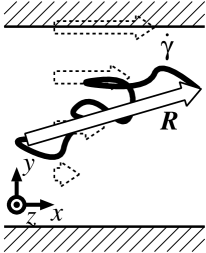
Figure 1:

Figure 2:

Figure 3:

Figure 4:

Figure 5:

References

- Kubo et al. (1991) R. Kubo, M. Toda, and N. Hashitsume, Statistical Physics II (Springer, Heidelberg, 1991).
- Evans and Morris (2008) D. J. Evans and G. P. Morris, Statistical Mechanics of Nonequilibrium Liquids, 2nd ed. (Cambridge University Press, Cambridge, 2008).
- Risken (1989) H. Risken, The Fokker-Planck Equation, 2nd ed. (Springer, Berlin, 1989).
- Doi and Edwards (1986) M. Doi and S. F. Edwards, The Theory of Polymer Dynamics (Oxford University Press, Oxford, 1986).
- Watanabe (1999) H. Watanabe, Prog. Polym. Sci. 24, 1253 (1999).
- Matsumiya et al. (2000) Y. Matsumiya, H. Watanabe, and K. Osaki, Macromolecules 33, 499 (2000).
- Watanabe et al. (2000) H. Watanabe, Y. Matsumiya, and K. Osaki, J. Polym. Sci. B: Polym. Phys. 38, 1024 (2000).
- Matsumiya and Watanabe (2001) Y. Matsumiya and H. Watanabe, Macromolecules 34, 5702 (2001).
- Watanabe et al. (2002a) H. Watanabe, Y. Matsumiya, and T. Inoue, Macromolecules 35, 2339 (2002a).
- Osaki et al. (1965) K. Osaki, M. Tamura, M. Kurata, and T. Kotaka, J. Phys. Chem. 69, 4183 (1965).
- de L. Costello (1997) B. A. de L. Costello, J. Non-Newtonian Fluid Mech. 68, 303 (1997).
- Vermant et al. (1998) J. Vermant, L. Walker, P. Moldenears, and J. Mewis, J. Non-Newtonian Fluid Mech. 79, 173 (1998).
- Isayev and Wong (1988) A. I. Isayev and C. M. Wong, J. Polym. Sci. B: Polym. Phys. 26, 2303 (1988).
- Wong and Isayev (1989) C. M. Wong and A. I. Isayev, Rheol. Acta 28, 176 (1989).
- Somma et al. (2007) E. Somma, O. Valentino, G. Titomanlio, and G. Ianniruberto, J. Rheol. 51, 987 (2007).
- Boukany and Wang (2009) P. E. Boukany and S.-Q. Wang, J. Rheol. 53, 1425 (2009).
- Li and Wang (2010) X. Li and S.-Q. Wang, Macromolecules 43, 5904 (2010).
- Matsumiya et al. (1998) Y. Matsumiya, H. Watanabe, T. Inoue, K. Osaki, and M.-L. Yao, Macromolecules 31, 7973 (1998).
- Watanabe et al. (1999) H. Watanabe, T. Sato, Y. Matsumiya, T. Inoue, and K. Osaki, Nihon Reoroji Gakkaishi (J. Soc. Rheol. Jpn.) 27, 121 (1999).
- Watanabe et al. (2002b) H. Watanabe, S. Ishida, and Y. Matsumiya, Macromolecules 35, 8802 (2002b).
- Watanabe et al. (2003a) H. Watanabe, Y. Matsumiya, and T. Inoue, J. Phys.: Cond. Matt. 15, S909 (2003a).
- Watanabe et al. (2005) H. Watanabe, Y. Matsumiya, and T. Inoue, Macromol. Symp. 228, 51 (2005).
- Uneyama et al. (2009) T. Uneyama, Y. Masubuchi, K. Horio, Y. Matsumiya, H. Watanabe, J. A. Pathak, and C. M. Roland, J. Polym. Sci. B: Polym. Phys. 47, 1039 (2009).
- Masubuchi et al. (2004) Y. Masubuchi, H. Watanabe, G. Ianniruberto, F. Greco, and G. Marrucci, Nihon Reoroji Gakkaishi (J. Soc. Rheol. Jpn.) 32, 192 (2004).
- Curtiss and Bird (1980a) C. F. Curtiss and R. B. Bird, J. Chem. Phys. 74, 2016 (1980a).
- Curtiss and Bird (1980b) C. F. Curtiss and R. B. Bird, J. Chem. Phys. 74, 2026 (1980b).
- Giesekus (1982) H. Giesekus, J. Non-Newtonian Fluid Mech. 11, 69 (1982).
- Arsac et al. (1994) A. Arsac, C. Carrot, J. Guillet, and P. Revenu, J. Non-Newtonian Fluid Mech. 55, 21 (1994).
- Stephanou et al. (2009) P. S. Stephanou, C. Baig, and V. G. Mavrantzas, J. Rheol. 53, 309 (2009).
- Beris and Edwards (1994) A. N. Beris and B. J. Edwards, Thermodynamics of Flowing Systems (Oxford University Press, Oxford, 1994).
- McPhie et al. (2001) M. G. McPhie, P. J. Daivis, I. K. Snook, J. Ennis, and D. J. Evans, Physica A 299, 412 (2001).
- Baiesi et al. (2009a) M. Baiesi, C. Maes, and B. Wynants, Phys. Rev. Lett. 103, 010602 (2009a).
- Baiesi et al. (2009b) M. Baiesi, C. Maes, and B. Wynants, J. Stat. Phys. 137, 1094 (2009b).
- Seifert and Speck (2001) U. Seifert and T. Speck, Europhys. Lett. 89, 10007 (2001).
- McLeish (2002) T. C. B. McLeish, Adv. Phys. 51, 1379 (2002).
- Kröger (2004) M. Kröger, Phys. Rep. 390, 453 (2004).
- Sarman et al. (1991) S. Sarman, D. J. Evans, and P. T. Cummings, J. Chem. Phys. 95, 8675 (1991).
- Evans (1991) D. J. Evans, Phys. Rev. A 44 (1991).
- Evans et al. (1992) D. J. Evans, A. Baranyai, and S. Sarman, Mol. Phys. 76 (1992).
- Sarman et al. (1992) S. Sarman, D. J. Evans, and A. Baranyai, Phys. Rev. A 46, 893 (1992).
- Hunt and Todd (2009) T. A. Hunt and B. D. Todd, J. Chem. Phys. 131, 054904 (2009).
- Kremer and Grest (1990) K. Kremer and G. S. Grest, J. Chem. Phys. 92, 5057 (1990).
- Baranyai (2000) A. Baranyai, Phys. Rev. E 62, 5989 (2000).
- Ilg (2010) P. Ilg, J. Non-Newtonian Fluid Mech. 165, 973 (2010).
- Ilg and Kröger (2011) P. Ilg and M. Kröger, J. Rheol. 55, 69 (2011).
- Johnson and Segalman (1977) M. W. Johnson and D. Segalman, J. Non-Newtonian Fluid Mech. 2, 255 (1977).
- Wu and Schümmer (1990) Q. Wu and P. Schümmer, Rheol. Acta 29, 23 (1990).
- Zylka and Öttinger (1989) W. Zylka and H. C. Öttinger, J. Chem. Phys. 90, 474 (1989).
- Wedgewood (1989) L. E. Wedgewood, J. Non-Newtonian Fluid Mech. 31, 127 (1989).
- Prabhakar and Prakash (2001) R. Prabhakar and J. R. Prakash, J. Rheol. 46, 1191 (2001).
- Graessley (1967) W. W. Graessley, J. Chem. Phys. 47, 1942 (1967).
- Macdonald and Bird (1966) I. F. Macdonald and R. B. Bird, J. Phys. Chem. 70, 2098 (1966).
- Tanner (1968) R. I. Tanner, Trans. Soc. Rheol. (J. Rheol.) 12, 155 (1968).
- Yamamoto (1971) M. Yamamoto, Trans. Soc. Rheol. (J. Rheol.) 15, 331 (1971).
- Marrucci (1996) G. Marrucci, J. Non-Newtonian Fluid Mech. 62, 279 (1996).
- Ianniruberto and Marrucci (1996) G. Ianniruberto and G. Marrucci, J. Non-Newtonian Fluid Mech. 65, 241 (1996).
- Mead et al. (1998) D. W. Mead, R. G. Larson, and M. Doi, Macromolecules 31, 7895 (1998).
- Ianniruberto and Marrucci (2001) G. Ianniruberto and G. Marrucci, J. Rheol. 45, 1305 (2001).
- Masubuchi et al. (2001) Y. Masubuchi, J. Takimoto, K. Koyama, G. Ianniruberto, F. Greco, and G. Marrucci, J. Chem. Phys. 115, 4387 (2001).
- Graham et al. (2003) R. S. Graham, A. E. Likhtman, T. C. B. McLeish, and S. T. Milner, J. Rheol. 47, 1171 (2003).
- Inoue and Osaki (1996) T. Inoue and K. Osaki, Macromolecules 29, 1595 (1996).
- Sridhar et al. (2000) T. Sridhar, D. A. Nguyen, and G. G. Fuller, J. Non-Newtonian Fluid Mech. 99, 299 (2000).
- Luap et al. (2005) C. Luap, C. Müller, T. Schweizer, and D. C. Venerus, Rheol. Acta 45, 83 (2005).
- Harada and Sasa (2005) T. Harada and S. Sasa, Phys. Rev. Lett. 95, 130602 (2005).
- Speck and Seifert (2006) T. Speck and U. Seifert, Europhys. Lett. 74, 391 (2006).
- Chetrite et al. (2008) R. Chetrite, G. Falkovich, and K. Gawȩdzki, J. Stat. Mech. 2008, P08005 (2008).
- Chetrite and Gawȩdzki (2009) R. Chetrite and K. Gawȩdzki, J. Stat. Phys. 137, 890 (2009).
- Ohta and Ohkuma (2008) T. Ohta and T. Ohkuma, J. Phys. Soc. Jpn. 77, 074004 (2008).
- Lebowitz and Spohn (1999) J. L. Lebowitz and H. Spohn, J. Stat. Phys. 95, 333 (1999).
- Qian (2001) H. Qian, Phys. Rev. E 65, 016102 (2001).
- Maes et al. (2008) C. Maes, K. Netočný, and B. Wynants, Physica A 387, 2675 (2008).
- Evans and Searles (2002) D. J. Evans and D. J. Searles, Adv. Phys. 51, 1529 (2002).
- Blickle et al. (2007) V. Blickle, T. Speck, C. Lutz, U. Siefert, and C. Bechinger, Phys. Rev. Lett. 98, 210601 (2007).
- Gomez-Solano et al. (2009) J. R. Gomez-Solano, A. Petrosyan, S. Ciliberto, R. Chetrite, and K. Gawȩdzki, Phys. Rev. Lett. 103, 040601 (2009).
- Marrucci (1985) G. Marrucci, J. Polym. Sci. B: Polym. Phys. 23, 159 (1985).
- Watanabe et al. (2003b) H. Watanabe, S. Ishida, Y. Matsumiya, and T. Inoue, Macromolecules 37, 6619 (2003b).
- Watanabe et al. (2006) H. Watanabe, T. Sawada, and Y. Matsumiya, Macromolecules 39, 2553 (2006).
- Watanabe (2008) H. Watanabe, Prog. Theor. Phys. Suppl. 175, 17 (2008).
- Shanbhag et al. (2001) S. Shanbhag, R. G. Larson, J. Takimoto, and M. Doi, Phys. Rev. Lett. 87, 195502 (2001).
- Phan-Thien et al. (1984) N. Phan-Thien, O. Manero, and L. G. Leal, Rheol. Acta 23 (1984).
- Baxandall (1987) L. G. Baxandall, J. Chem. Phys. 87, 2297 (1987).
- Biller and Petruccione (1988) P. Biller and F. Petruccione, J. Chem. Phys. 89, 2412 (1988).
- Likhtman (2005) A. E. Likhtman, Macromolecules 38, 6128 (2005).
- Gordon and Schowalter (1972) R. J. Gordon and W. R. Schowalter, Trans. Soc. Rheol. (J. Rheol.) 16, 79 (1972).
- Gardiner (2004) C. W. Gardiner, Handbook of Stochastic Methods, 3rd ed. (Springer, Berlin, 2004).
- Kleinert (2004) H. Kleinert, Path Integrals in Quantum Mechanics, Statistics, Polymer Physics, and Finantial Markets, 3rd ed. (World Scientific, Singapore, 2004).