Causal signal transmission by quantum fields.
Phase-space approach to quantum electrodynamics.

Abstract

Phase-space techniques are generalised to nonlinear quantum electrodynamics beyond the rotating wave approximation, resulting in an essentially classical picture of radiation dynamics.

This is an early version of Plimak et al. (2015), with a number of formal details omitted there.

I Introduction

The goal of this paper is to generalise phase-space techniques to nonlinear quantum electrodynamics. A systematic introduction to conventional phase-space concepts may be found, e.g., in Mandel and Wolf Wolf and Mandel (1995). For our methods we owe a lot to Agarwal and Wolf Agarwal and Wolf (1970). It is advisable for the reader to familiarise himself with section II of our paper Plimak and Stenholm (2011a) before continuing with this one.

Coherent states of the harmonic oscillator, which traditionally serve as an entry point to phase-space approaches, were introduced by Schrödinger as early as 1926 Schrödinger (1926). That quantum dynamics of free bosonic systems maps to classical dynamics irrespective of the quantum state was firstly noticed by Feynman in his review on path integrals Feynman (1948). This understanding was instrumental in developing quantum theory of photodetection by Glauber Glauber (1963). Glauber’s theory was initially formulated for free electromagnetic fields. It was extended to interacting fields by Kelley and Kleiner Kelley and Kleiner (1964); Glauber (1965). However, de Haan de Haan (1985) and later Bykov and Tatarskii Bykov and Tatarskii (1989); Tatarskii (1990) pointed out that Kelley-Kleiner’s results are limited to the resonance, or rotating wave, approximation (RWA). Taking them outside the RWA leads to causality violations. In this paper, we lift this last restriction, generalising phase-space concepts to an arbitrary case of electromagnetic interaction.

Our approach Plimak and Stenholm (2008a, b, 2009, 2011b, 2011a) (see also Refs. Belinicher and Tikhodeev (1988); Plimak (1994); Plimak et al. (2003)) hinges on explicit causality as a guiding principle. It originates in the observation that the commutator of free electromagnetic-field operators depends only on the linear response function, or, which is the same, retarded Green function, of the free field. In Ref. Plimak (1994) the formula relating commutator to response was called the wave quantisation relation. In Ref. Plimak and Stenholm (2008a), we demonstrated that the wave quantisation relation leads to the so called response transformation of linear quantum dynamics. It was shown that the latter serves as an alternative entry point to conventional phase-space approaches, revealing the profound connection between causality (inherent in response of the field) and such formal concepts as normal ordering of bosonic operators. In Refs. Plimak and Stenholm (2008b, 2009), we postulated response transformations for Heisenberg field operators and showed that it results in a natural response formulation of quantum fields, which is at the same time a phase-space formulation generalised beyond the RWA.

Analyses in Ref. Plimak and Stenholm (2008a) were limited to linear systems, while those in Refs. Plimak and Stenholm (2008b, 2009) were to a large extent kinematical. Response transformation of nonlinear quantum dynamics was developed in Refs. Plimak and Stenholm (2011b, a). In Ref. Plimak and Stenholm (2011b) we applied response transformation to Wick’s theorem. The emerging relations were called causal Wick theorems. In Ref. Plimak and Stenholm (2011a) the causal Wick theorem for the electromagnetic field was combined with Dyson’s standard perturbative approach of quantum field theory Schweber (2005). In this paper, we put results of Refs. Plimak and Stenholm (2008a, b, 2009, 2011b, 2011a) together. We encounter perfect consistency of generalised phase-space concepts introduced in Refs. Plimak and Stenholm (2008b, 2009) with quantum dynamics in response representation devised in Refs. Plimak and Stenholm (2011b, a) — not quite unexpectedly, given that all results are ultimately due to the wave quantisation formula.

The result of this paper in a nutshell is that, expressed in phase-space terms, dynamics of the electromagnetic field becomes classical. In particular, propagation of the field in space and time is always subject to strict causality. Formally, this is due to properties of the free field (ultimately, to Feynman’s observation) and to the bilinear structure of the electromagnetic interaction.

The paper is organised as follows. In section II we recall conventional Kelley and Kleiner (1964); Glauber (1965) and amended Plimak and Stenholm (2008b, 2009) definitions of the time-normal ordering. In section III, we reiterate results of Ref. Plimak and Stenholm (2011a). Sections IV and V are concerned with parallelism between classical stochastic and quantum electrodynamics. In section IV, we rewrite results of Ref. Plimak and Stenholm (2011a) in terms of time-normally ordered operator averages, and show that this leads to an essentially classical picture of electromagnetic interactions. In section V, we introduce the concept of P-functional, which generalises the conventional P-function Wolf and Mandel (1995) to multitime quantum averages of Heisenberg operators, and show that any relation for time-normal operator averages and P-functionals coincides with some relation for classical stochastic averages and probability distributions. In section VI we demonstrate that P-functionals also give a natural, and in essense classical, insight into the electromagnetic self-action (“dressing”) problem. In section VII we briefly discuss mathematical complications hidden behind the apparent simplicity of our formulae. The appendix is concerned with functional probability distributions and related issues.

II Time-normal ordering of operators

II.1 Preliminary remarks

We start from refreshing our memory on the concepts of time-normal operator product and time-normal average. As in Ref. Plimak and Stenholm (2011a) we distinguish the narrow-band and broad-band case s, which differ in whether the resonance, or rotating wave, approximation (RWA) is or is not made in dynamics. In the narrow-band case, definition of the time-normal ordering follows Kelley and Kleiner Kelley and Kleiner (1964); Glauber (1965). In the broad-band case, we adhere to the amended definition of Refs. Plimak and Stenholm (2008b, 2009). For formal justifications and discussions see Refs. Plimak and Stenholm (2008a, b, 2009, 2011b, 2011a) (cf. also Refs. Plimak (1994); Plimak et al. (2003)).

To be specific, we talk about the Heisenberg dipole-momentum operator ${\hat{\mathcal{D}}}(t)$ and its Hermitian-adjoint ${\hat{\mathcal{D}}}^{{\dagger}}(t)$ in the narrow-band case, and about the Heisenberg current operator ${\hat{\mathcal{J}}}(t)$ in the broad-band case. For brevity we drop all arguments of the operators except time. As dynamical quantities, the dipole and current operators will be defined in section III.1. For purposes of this section, their physical nature is irrelevant. Hermiticity of ${\hat{\mathcal{J}}}(t)$ does not matter either, with the only exception of reality conditions in section II.4.

II.2 The narrow-band case

In the narrow-band case, time-normal operator ordering is an operation which places all ${\hat{\mathcal{D}}}^{{\dagger}}(t)$’s to the left of all ${\hat{\mathcal{D}}}(t)$’s. Among themselves, the ${\hat{\mathcal{D}}}(t)$ operators are time-ordered, which means setting them from left to right in the order of decreasing time arguments. The ${\hat{\mathcal{D}}}^{{\dagger}}(t)$ operators are reverse-time-ordered, which means setting them from left to right in the order of increasing time arguments. These two types of time-ordering are denoted as $T_{+}$ and $T_{-}$, respectively. That is,

$$\hskip 86.72267pt{\mathcal{T}}{\mbox{\rm\boldmath$:$}}{\hat{\mathcal{D}}}^{{\dagger}}(t_{1})\cdots{\hat{\mathcal{D}}}^{{\dagger}}(t_{m}){\hat{\mathcal{D}}}(t_{1}^{\prime})\cdots{\hat{\mathcal{D}}}(t_{n}^{\prime}){\mbox{\rm\boldmath$:$}}\\ =T_{-}{\hat{\mathcal{D}}}^{{\dagger}}(t_{1})\cdots{\hat{\mathcal{D}}}^{{\dagger}}(t_{m})\,T_{+}{\hat{\mathcal{D}}}(t_{1}^{\prime})\cdots{\hat{\mathcal{D}}}(t_{n}^{\prime}).\hskip 86.72267pt$$ (1)

The notation ${\mathcal{T}}{\mbox{\rm\boldmath$:$}}\cdots{\mbox{\rm\boldmath$:$}}$ for the time-normal ordering is borrowed from Mandel and Wolf Wolf and Mandel (1995).

In quantum field theory and condensed matter physics Schwinger (1961); Konstantinov and Perel (1960); Keldysh (1964), the double-time-ordered structure as in (1) is commonly expressed as a closed-time-loop, or C-contour, ordering, which we denote $T_{C}$. Formally, one marks operators under the $T_{\pm}$-orderings by _± indices, and allows them to commute freely. So, eq. (1) in terms of the $T_{C}$-ordering becomes,

$$\hskip 86.72267pt{\mathcal{T}}{\mbox{\rm\boldmath$:$}}{\hat{\mathcal{D}}}^{{\dagger}}(t_{1})\cdots{\hat{\mathcal{D}}}^{{\dagger}}(t_{m}){\hat{\mathcal{D}}}(t_{1}^{\prime})\cdots{\hat{\mathcal{D}}}(t_{n}^{\prime}){\mbox{\rm\boldmath$:$}}\\ =T_{C}{\hat{\mathcal{D}}}_{-}^{{\dagger}}(t_{1})\cdots{\hat{\mathcal{D}}}_{-}^{{\dagger}}(t_{m}){\hat{\mathcal{D}}}_{+}(t_{1}^{\prime})\cdots{\hat{\mathcal{D}}}_{+}(t_{n}^{\prime}),\\ =T_{C}{\hat{\mathcal{D}}}_{+}(t_{1}^{\prime})\cdots{\hat{\mathcal{D}}}_{+}(t_{n}^{\prime}){\hat{\mathcal{D}}}_{-}^{{\dagger}}(t_{1})\cdots{\hat{\mathcal{D}}}_{-}^{{\dagger}}(t_{m}).\hskip 86.72267pt$$ (2)

etc. For more details see, e.g., our Ref. Plimak and Stenholm (2009).

Of actual interest to us are the time-normal averages of the dipole operators,

$$\hskip 86.72267pt\big{\langle}{\mathcal{T}}{\mbox{\rm\boldmath$:$}}{\hat{\mathcal{D}}}^{{\dagger}}(t_{1})\cdots{\hat{\mathcal{D}}}^{{\dagger}}(t_{m}){\hat{\mathcal{D}}}(t_{1}^{\prime})\cdots{\hat{\mathcal{D}}}(t_{n}^{\prime}){\mbox{\rm\boldmath$:$}}\big{\rangle}\\ =\frac{i^{m}(-i)^{n}\delta^{m+n}\Phi\big{(}\nu,\nu^{*}\big{)}}{\delta\nu(t_{1})\cdots\delta\nu(t_{m})\delta\nu^{*}(t^{\prime}_{1})\cdots\delta\nu^{*}(t^{\prime}_{n})}\raisebox{-2.70003pt}{$\big{|}_{\nu=0}$}.\hskip 86.72267pt$$ (3)

We have immediately introduced their generating, or characteristic, functional,

$$\hskip 86.72267pt\Phi\big{(}\nu,\nu^{*}\big{)}=\bigg{\langle}{\mathcal{T}}{\mbox{\rm\boldmath$:$}}\exp\bigg{\{}i\int dt\big{[}\nu^{*}(t){\hat{\mathcal{D}}}(t)-\nu(t){\hat{\mathcal{D}}}^{{\dagger}}(t)\big{]}\bigg{\}}{\mbox{\rm\boldmath$:$}}\bigg{\rangle}\\ =\bigg{\langle}T_{C}\exp\bigg{\{}i\int dt\big{[}\nu^{*}(t){\hat{\mathcal{D}}}_{+}(t)-\nu(t){\hat{\mathcal{D}}}_{-}^{{\dagger}}(t)\big{]}\bigg{\}}\bigg{\rangle},\hskip 86.72267pt$$ (4)

where $\nu(t)$ is an auxiliary complex c-number function. The same in terms of the double-time-ordering reads,

$$\hskip 86.72267pt\Phi\big{(}\nu,\nu^{*}\big{)}=\bigg{\langle}T_{-}\exp\bigg{[}-i\int dt\nu(t){\hat{\mathcal{D}}}^{{\dagger}}(t)\bigg{]}\\ \times T_{+}\exp\bigg{[}i\int dt\nu^{*}(t){\hat{\mathcal{D}}}(t)\bigg{]}\bigg{\rangle}.\hskip 86.72267pt$$ (5)

The averaging in eqs. (3)–(5) is over the initial (Heisenberg) state of the system,

$${{\begin{aligned} \big{\langle}\cdots\big{\rangle}=\text{Tr}\hat{\rho}(\cdots),\end{aligned}}}$$ (6)

where the ellipsis stands for an arbitrary operator. Unlike in Refs. Plimak and Stenholm (2008a, b, 2009); Plimak et al. (2003), we define (4) with a complex-conjugate pair of arguments $\nu(t),\nu^{*}(t)$ in place of a pair of independent functions $\nu(t),\bar{\nu}(t)$. The reason for this was clarified in Plimak and Stenholm (2011a), section VB.

A word of extreme caution is in place here. The time-normal ordering (1), (2) is defined only for products of (more generally speaking, for quantities that may be regarded functionals of) ${\hat{\mathcal{D}}}(t),{\hat{\mathcal{D}}}^{{\dagger}}(t)$. Ignoring this reservation leads to confusion and plain nonsense. For example, in physical models, dipole operators are commonly defined as,

$${{\begin{aligned} {\hat{\mathcal{D}}}(t)=\hat{\psi}^{{\dagger}}_{\mathrm{g}}(t)\hat{\psi}_{\mathrm{e}}(t),\end{aligned}}}$$ (7)

where $\hat{\psi}^{{\dagger}}_{\mathrm{g}}(t)$ and $\hat{\psi}_{\mathrm{e}}(t)$ are creation and annihilation operators for the ground and excited states (say) of an atom. Definitions like (1), (2) may then be given for the atomic operators. To maintain rigour, one has to introduce two symbols, e.g., $\mathcal{T}^{{\hat{\mathcal{D}}}}{\mbox{\rm\boldmath$:$}}\cdots{\mbox{\rm\boldmath$:$}}$ and $\mathcal{T}^{\hat{\psi}}{\mbox{\rm\boldmath$:$}}\cdots{\mbox{\rm\boldmath$:$}}$, for time-normal orderings with respect to dipole momenta and to atomic operators. Then, for the dipole operators,

$$\hskip 86.72267pt\mathcal{T}^{{\hat{\mathcal{D}}}}{\mbox{\rm\boldmath$:$}}{\hat{\mathcal{D}}}^{{\dagger}}(t){\hat{\mathcal{D}}}(t^{\prime}){\mbox{\rm\boldmath$:$}}={\hat{\mathcal{D}}}^{{\dagger}}(t){\hat{\mathcal{D}}}(t^{\prime})\\ =\hat{\psi}^{{\dagger}}_{\mathrm{g}}(t)\hat{\psi}_{\mathrm{e}}(t)\hat{\psi}^{{\dagger}}_{\mathrm{g}}(t^{\prime})\hat{\psi}_{\mathrm{e}}(t^{\prime}),\hskip 86.72267pt$$ (8)

whereas for the atomic operators end ,

$$\hskip 86.72267pt\mathcal{T}^{\hat{\psi}}{\mbox{\rm\boldmath$:$}}{\hat{\mathcal{D}}}^{{\dagger}}(t){\hat{\mathcal{D}}}(t^{\prime}){\mbox{\rm\boldmath$:$}}=\mathcal{T}^{\hat{\psi}}{\mbox{\rm\boldmath$:$}}\hat{\psi}^{{\dagger}}_{\mathrm{g}}(t)\hat{\psi}_{\mathrm{e}}(t)\hat{\psi}^{{\dagger}}_{\mathrm{g}}(t^{\prime})\hat{\psi}_{\mathrm{e}}(t^{\prime}){\mbox{\rm\boldmath$:$}}\\ =\bar{T}\hat{\psi}^{{\dagger}}_{\mathrm{g}}(t^{\prime})\hat{\psi}^{{\dagger}}_{\mathrm{g}}(t)\,T\hat{\psi}_{\mathrm{e}}(t)\hat{\psi}_{\mathrm{e}}(t^{\prime}).\hskip 86.72267pt$$ (9)

These two quantities are distinct for $t\neq t^{\prime}$ (recall that ${\hat{\mathcal{D}}}(t),\hat{\psi}_{\mathrm{g}}(t),\hat{\psi}_{\mathrm{e}}(t)$ are Heisenberg operators). By ignoring the difference between $\mathcal{T}^{{\hat{\mathcal{D}}}}{\mbox{\rm\boldmath$:$}}\cdots{\mbox{\rm\boldmath$:$}}$ and $\mathcal{T}^{\hat{\psi}}{\mbox{\rm\boldmath$:$}}\cdots{\mbox{\rm\boldmath$:$}}$ one can “prove” that quantities (8) and (9) coincide. This is one example of the aforementioned “plain nonsense.” Similar reservations apply to other cases of time-normal ordering.

II.3 The broad-band case

In the broad-band case, the time-normal averages of the current operator are defined through their generating functional,

$${{\begin{aligned} \big{\langle}{\mathcal{T}}{\mbox{\rm\boldmath$:$}}{\hat{\mathcal{J}}}(t_{1})\cdots{\hat{\mathcal{J}}}(t_{m}){\mbox{\rm\boldmath$:$}}\big{\rangle}=\frac{(-i)^{m}\delta^{m}\Phi\big{(}\zeta\big{)}}{\delta\zeta(t_{1})\cdots\delta\zeta(t_{m})}\raisebox{-2.70003pt}{$\big{|}_{\zeta=0}$},\end{aligned}}}$$ (10)

which is postulated to be Plimak and Stenholm (2008a, b, 2009),

$$\hskip 86.72267pt\Phi(\zeta)\equiv\bigg{\langle}{\mathcal{T}}{\mbox{\rm\boldmath$:$}}\exp\bigg{[}i\int dt\zeta(t){\hat{\mathcal{J}}}(t)\bigg{]}{\mbox{\rm\boldmath$:$}}\bigg{\rangle}\\ =\bigg{\langle}T_{C}\exp\bigg{\{}i\int dt\big{[}\zeta^{(-)}(t){\hat{\mathcal{J}}}_{+}(t)+\zeta^{(+)}(t){\hat{\mathcal{J}}}_{-}(t)\big{]}\bigg{\}}\bigg{\rangle}.\hskip 86.72267pt$$ (11)

The symbols ^(±) denote separation of the frequency-positive and negative parts of functions,

$${{\begin{aligned} &f(t)=f^{(+)}(t)+f^{(-)}(t),\\ &f^{(\pm)}(t)=\int_{-\infty}^{+\infty}\frac{d\omega}{2\pi}\mathrm{e}^{-i\omega t}\theta(\pm\omega)f_{\omega},&&f_{\omega}=\int_{-\infty}^{+\infty}dt\mathrm{e}^{i\omega t}f(t).\end{aligned}}}$$ (12)

This operation is alternatively expressed as an integral transformation,

$${{\begin{aligned} f^{(\pm)}(t)=\int dt^{\prime}\delta^{(\pm)}(t-t^{\prime})f(t^{\prime}),\end{aligned}}}$$ (13)

where

$${{\begin{aligned} \delta^{(\pm)}(t)=\delta^{(\mp)}(-t)=\big{[}\delta^{(\mp)}(t)\big{]}^{*}=\pm\frac{1}{2\pi i(t\mp i0^{+})}\end{aligned}}}$$ (14)

are the frequency-positive and negative parts of the delta-function. For more details on this operation see Ref. Plimak and Stenholm (2008b), appendix A.

Accounting for (13), eq. (11) reads,

$$\hskip 86.72267pt\Phi(\zeta)=\bigg{\langle}T_{C}\exp\bigg{\{}i\int dtdt^{\prime}\zeta(t)\Big{[}\delta^{(-)}(t-t^{\prime}){\hat{\mathcal{J}}}_{-}(t^{\prime})\\ +\delta^{(+)}(t-t^{\prime}){\hat{\mathcal{J}}}_{+}(t^{\prime})\Big{]}\bigg{\}}\bigg{\rangle}.\hskip 86.72267pt$$ (15)

Differentiating (15) as per eq. (10) we find the explicit formula,

$$\hskip 86.72267pt\big{\langle}{\mathcal{T}}{\mbox{\rm\boldmath$:$}}{\hat{\mathcal{J}}}(t_{1})\cdots{\hat{\mathcal{J}}}(t_{m}){\mbox{\rm\boldmath$:$}}\big{\rangle}\\ =\bigg{\langle}T_{C}\int dt^{\prime}_{1}\cdots dt^{\prime}_{m}\prod_{l=1}^{m}\Big{[}\delta^{(-)}(t_{l}-t^{\prime}_{l}){\hat{\mathcal{J}}}_{-}(t^{\prime}_{l})\\ +\delta^{(+)}(t_{l}-t^{\prime}_{l}){\hat{\mathcal{J}}}_{+}(t^{\prime}_{l})\Big{]}\bigg{\rangle}.\hskip 86.72267pt$$ (16)

The GKK definition is recovered applying separation of the frequency-positive and negative parts to the operators,

$$\hskip 86.72267pt\big{\langle}{\mathcal{T}}{\mbox{\rm\boldmath$:$}}{\hat{\mathcal{J}}}(t_{1})\cdots{\hat{\mathcal{J}}}(t_{m}){\mbox{\rm\boldmath$:$}}\big{\rangle}\raisebox{-2.25002pt}{$|_{\mathrm{GKK}}$}\\ =\bigg{\langle}T_{C}\prod_{l=1}^{m}\big{[}{\hat{\mathcal{J}}}^{(-)}_{-}(t_{l})+{\hat{\mathcal{J}}}^{(+)}_{+}(t_{l})\big{]}\bigg{\rangle},\ \ \mathrm{(RWA\ only)}\hskip 86.72267pt$$ (17)

which coincides with (1) up to the replacements,

$${{\begin{aligned} &{\hat{\mathcal{J}}}^{(+)}(t)\leftrightarrow{\hat{\mathcal{D}}}(t),&&{\hat{\mathcal{J}}}^{(-)}(t)\leftrightarrow{\hat{\mathcal{D}}}^{{\dagger}}(t).\end{aligned}}}$$ (18)

In general, eq. (17) is incorrect, because separation of the frequency-positive and negative parts in (16) applies to $T_{C}$-ordered products of the operators and not to the operators themselves. It becomes a valid approximation under the RWA. For a detailed discussion see Refs. Plimak and Stenholm (2008b, 2011a).

II.4 Reality and causality

Consistency of all physical interpretations in this paper hinge on reality and causality properties of time-normal products and averages. Using that Hermitian conjugation reverts the order of operators we find,

$$\hskip 86.72267pt\big{[}{\mathcal{T}}{\mbox{\rm\boldmath$:$}}\hat{D}^{{\dagger}}(t_{1})\cdots\hat{D}^{{\dagger}}(t_{m})\hat{D}(t_{1}^{\prime})\cdots\hat{D}(t_{n}^{\prime}){\mbox{\rm\boldmath$:$}}\big{]}^{{\dagger}}\\ ={\mathcal{T}}{\mbox{\rm\boldmath$:$}}\hat{D}(t_{1})\cdots\hat{D}(t_{m})\hat{D}^{{\dagger}}(t_{1}^{\prime})\cdots\hat{D}^{{\dagger}}(t_{n}^{\prime}){\mbox{\rm\boldmath$:$}}.\hskip 86.72267pt$$ (19)

Adding eq. (14) to the argument and assuming Hermiticity of ${\hat{\mathcal{J}}}(t)$ it is also straightforward to show that,

$${{\begin{aligned} \big{[}{\mathcal{T}}{\mbox{\rm\boldmath$:$}}{\hat{\mathcal{J}}}(t_{1})\cdots{\hat{\mathcal{J}}}(t_{m}){\mbox{\rm\boldmath$:$}}\big{]}^{{\dagger}}={\mathcal{T}}{\mbox{\rm\boldmath$:$}}{\hat{\mathcal{J}}}(t_{1})\cdots{\hat{\mathcal{J}}}(t_{m}){\mbox{\rm\boldmath$:$}}.\end{aligned}}}$$ (20)

The time-normal averages of the current operator are therefore real,

$${{\begin{aligned} \big{\langle}{\mathcal{T}}{\mbox{\rm\boldmath$:$}}{\hat{\mathcal{J}}}(t_{1})\cdots{\hat{\mathcal{J}}}(t_{m}){\mbox{\rm\boldmath$:$}}\big{\rangle}^{*}=\big{\langle}{\mathcal{T}}{\mbox{\rm\boldmath$:$}}{\hat{\mathcal{J}}}(t_{1})\cdots{\hat{\mathcal{J}}}(t_{m}){\mbox{\rm\boldmath$:$}}\big{\rangle},\end{aligned}}}$$ (21)

while those of the dipole operators obey the natural property,

$$\hskip 86.72267pt\big{\langle}{\mathcal{T}}{\mbox{\rm\boldmath$:$}}\hat{D}^{{\dagger}}(t_{1})\cdots\hat{D}^{{\dagger}}(t_{m})\hat{D}(t_{1}^{\prime})\cdots\hat{D}(t_{n}^{\prime}){\mbox{\rm\boldmath$:$}}\big{\rangle}^{*}\\ =\big{\langle}{\mathcal{T}}{\mbox{\rm\boldmath$:$}}\hat{D}(t_{1})\cdots\hat{D}(t_{m})\hat{D}^{{\dagger}}(t_{1}^{\prime})\cdots\hat{D}^{{\dagger}}(t_{n}^{\prime}){\mbox{\rm\boldmath$:$}}\big{\rangle}.\hskip 86.72267pt$$ (22)

As to causality, the following “no-peep-into-the-future” theorem holds: a time-normal product depends on the Heisenberg operators it comprises only for times not later than the latest time argument of these operators Plimak and Stenholm (2011c). If dependence of some operators on a perturbation is causal, dependence of their time-normal products on this perturbation is also causal. The question of causality of time-normal products reduces to that of quantum equations of motion. The “no-peep-into-the-future theorem” extends the causality conditions verified in Plimak and Stenholm (2008b) from additive external sources in equations of motion to arbitrary perturbations. It holds trivially in the narrow-band case, but becomes nontrivial in the broad-band case, because separation of the frequency-positive and negative parts smears functions all over the time axis. In fact, the “future tail” in eq. (16) cancels. For a proof see Ref. Plimak and Stenholm (2011c).

III Quantum electrodynamics in response representation revisited

III.1 The Hamiltonian

In this section, we reiterate key results of our previous paper Plimak and Stenholm (2011a). In Ref. Plimak and Stenholm (2011a), we considered a quantum device interacting with a collection of oscillator modes, with the Hamiltonian in the interaction picture being,

$${{\begin{aligned} &\hat{H}(t)=\hbar\sum_{\kappa=1}^{N}\omega_{\kappa}\hat{a}_{\kappa}^{{\dagger}}\hat{a}_{\kappa}+\hat{H}_{\mathrm{dev}}(t)+\hat{H}_{\text{I}}(t).\end{aligned}}}$$ (23)

The oscillators, represented by the standard creation and annihilation operators,

$${{\begin{aligned} &\big{[}\hat{a}_{\kappa},\hat{a}_{\kappa^{\prime}}^{{\dagger}}\big{]}=\delta_{k\kappa^{\prime}},&&\kappa,\kappa^{\prime}=1,\cdots,N.\end{aligned}}}$$ (24)

are organised in two quantised fields,

$$\hat{E}(x,t) =i\sum_{\kappa=1}^{M}\sqrt{\frac{\hbar\omega_{\kappa}}{2}}u_{\kappa}(x)\hat{a}_{\kappa}\mathrm{e}^{-i(\omega_{\kappa}-\omega_{0})t},$$ (25)

$$\hat{E}^{{\dagger}}(x,t) =-i\sum_{\kappa=1}^{M}\sqrt{\frac{\hbar\omega_{\kappa}}{2}}u^{*}_{\kappa}(x)\hat{a}_{\kappa}^{{\dagger}}\mathrm{e}^{i(\omega_{\kappa}-\omega_{0})t},$$

$$\hat{A}(x,t) =\sum_{\kappa=M+1}^{N}\sqrt{\frac{\hbar}{2\omega_{\kappa}}}u_{\kappa}(x)\hat{a}_{\kappa}\mathrm{e}^{-i\omega_{\kappa}t}+\mathrm{H.c.}\,,$$ (26)

where $u_{k}(x)$ are complex mode functions, and variable $x$ comprises all field arguments except time. Electromagnetic interaction in (23) is split accordingly,

$${{\begin{aligned} \hat{H}_{\text{I}}(t)=\hat{H}_{\text{I}}^{(1)}(t)+\hat{H}_{\text{I}}^{(2)}(t).\end{aligned}}}$$ (27)

The narrow-band, or resonant, field $\hat{E}(x,t)$ interacts with the device according to the resonant Hamiltonian,

$$\hskip 86.72267pt\hat{H}_{\text{I}}^{(1)}(t)=-\int dx\big{[}\hat{D}(x,t)\hat{E}^{{\dagger}}(x,t)+\hat{D}(x,t)E^{*}_{\mathrm{e}}(x,t)\\ +D_{\mathrm{e}}(x,t)\hat{E}^{{\dagger}}(x,t)\big{]}+\mathrm{H.c.}\,,\hskip 86.72267pt$$ (28)

while the broad-band, or nonresonant, field $\hat{A}(x,t)$ — according to the nonresonant Hamiltonian,

$$\hskip 86.72267pt\hat{H}_{\text{I}}^{(2)}(t)=-\int dx\big{[}\hat{J}(x,t)\hat{A}(x,t)+\hat{J}(x,t)A_{\mathrm{e}}(x,t)\\ +J_{\mathrm{e}}(x,t)\hat{A}(x,t)\big{]}.\hskip 86.72267pt$$ (29)

The Hamiltonian $\hat{H}_{\mathrm{dev}}(t)$, the dipole momentum $\hat{D}(x,t)$ and the current operator $\hat{J}(x,t)$ describe the device. They commute with $\hat{a}_{\kappa},\hat{a}_{\kappa}^{{\dagger}}$ and otherwise remain arbitrary. The initial state of all oscillators is vacuum, while that of the device is also arbitrary. The c-number external sources $E_{\mathrm{e}}(x,t)$, $D_{\mathrm{e}}(x,t)$, $A_{\mathrm{e}}(x,t)$, and $J_{\mathrm{e}}(x,t)$ are added for formal purposes.

Hamiltonian (23) may be adjusted to any conceivable case of electromagnetic interaction. From our perspective, this Hamiltonian is a structural model of a quantum-optical experiment involving photodetection. For justification and discussion of this model see sections II and III in Ref. Plimak and Stenholm (2011a).

III.2 Condensed notation

To keep the bulk of formulae under the lid and make their structure more transparent, we make extensive use of condensed notation,

$$fg=\int dxdtf(x,t)g(x,t),$$ (30)

$$fKg=\int dxdx^{\prime}dtdt^{\prime}f(x,t)K(x,x^{\prime},t-t^{\prime})g(x^{\prime},t^{\prime}),$$ (31)

$$(Kg)(x,t)=\int dx^{\prime}dt^{\prime}K(x,x^{\prime},t-t^{\prime})g(x^{\prime},t^{\prime}),$$ (32)

$$(fK)(x,t)=\int dx^{\prime}dt^{\prime}g(x^{\prime},t^{\prime})K(x^{\prime},x,t^{\prime}-t),$$ (33)

where $f(x,t)$ and $g(x,t)$ are c-number or q-number functions, and $K(x,x^{\prime},t-t^{\prime})$ is a c-number kernel. The “products” $fg$ and $fKg$ denote scalars, while $Kg$ and $fK$ — functions (fields).

III.3 Closed-time-loop formalism and response transformation

Fields, currents and dipoles in eqs. (25)–(29) are interaction-picture operators. Their Heisenberg counterparts will be denoted by calligraphic letters as ${\hat{\mathcal{E}}}(x,t)$, ${\hat{\mathcal{A}}}(x,t)$, ${\hat{\mathcal{D}}}(x,t)$, and ${\hat{\mathcal{J}}}(x,t)$. We solve for the characteristic functional of the $T_{C}$-ordered products of the Heisenberg operators written in causal variables,

$$\Phi\big{(}\eta,\mu,\mu^{*},\zeta,\nu,\nu^{*}\big{|}j_{\mathrm{e}},d_{\mathrm{e}},d_{\mathrm{e}}^{*},a_{\mathrm{e}},e_{\mathrm{e}},e_{\mathrm{e}}^{*}\big{|}J_{\mathrm{e}},D_{\mathrm{e}},D_{\mathrm{e}}^{*},A_{\mathrm{e}},E_{\mathrm{e}},E_{\mathrm{e}}^{*}\big{)}\\ =\Big{\langle}T_{C}\exp\big{(}i{\eta}_{+}{\hat{\mathcal{A}}}_{+}-i{\eta}_{-}{\hat{\mathcal{A}}}_{-}+i{\zeta}_{+}{\hat{\mathcal{J}}}_{+}-i{\zeta}_{-}{\hat{\mathcal{J}}}_{-}\big{)}\\ \times\exp\big{(}i\bar{\mu}_{+}{\hat{\mathcal{E}}}_{+}+i\mu_{+}{\hat{\mathcal{E}}}_{+}^{{\dagger}}-i\bar{\mu}_{-}{\hat{\mathcal{E}}}_{-}-i\mu_{-}{\hat{\mathcal{E}}}_{-}^{{\dagger}}+i\bar{\nu}_{+}{\hat{\mathcal{D}}}_{+}+i\nu_{+}{\hat{\mathcal{D}}}_{+}^{{\dagger}}-i\bar{\nu}_{-}{\hat{\mathcal{D}}}_{-}-i\nu_{-}{\hat{\mathcal{D}}}_{-}^{{\dagger}}\big{)}\Big{\rangle}\raisebox{-2.70003pt}{$\big{|}_{\mathrm{c.v.}}$},$$ (34)

where $\eta_{\pm}(x,t)$, $\zeta_{\pm}(x,t)$, $\mu_{\pm}(x,t)$, $\bar{\mu}_{\pm}(x,t)$, $\nu_{\pm}(x,t)$, and $\bar{\nu}_{\pm}(x,t)$ in (34) are auxiliary complex c-number functions, and c.v. refers to the set of response substitutions, (with arguments dropped for clarity)

$${{\begin{aligned} \eta_{\pm}&=\frac{j_{\mathrm{e}}}{\hbar}\pm\eta^{(\mp)},&\zeta_{\pm}&=\frac{a_{\mathrm{e}}}{\hbar}\pm\zeta^{(\mp)},\\ \mu_{+}&=\frac{d_{\mathrm{e}}}{\hbar},&\bar{\mu}_{+}&=\mu^{*}+\frac{d_{\mathrm{e}}^{*}}{\hbar},&\bar{\mu}_{-}&=\frac{d_{\mathrm{e}}^{*}}{\hbar},&\mu_{-}&=\mu+\frac{d_{\mathrm{e}}}{\hbar},\\ \nu_{+}&=\frac{e_{\mathrm{e}}}{\hbar},&\bar{\nu}_{+}&=\nu^{*}+\frac{e_{\mathrm{e}}^{*}}{\hbar},&\bar{\nu}_{-}&=\frac{e_{\mathrm{e}}^{*}}{\hbar},&\nu_{-}&=\nu+\frac{e_{\mathrm{e}}}{\hbar}.\end{aligned}}}$$ (35)

We use notation (30). The symbols ^(±) denote separation of the frequency-positive and negative parts, cf. eq. (12). $T_{C}$-ordering was defined in section II.2. The averaging in (34) is over the initial (Heisenberg) state of the system, cf. eq. (6). We remind that the initial state of all oscillators is vacuum,

$${{\begin{aligned} \hat{\rho}=\hat{\rho}_{\mathrm{dev}}\otimes\big{|}0\big{\rangle}\big{\langle}0\big{|},\end{aligned}}}$$ (36)

Not to be lost in these definitions, note the following. The Heisenberg operators are by construction dependent (conditional) on the sources; in (34), this dependence is made explicit. Furthermore, operators in (34) are organised in repetitive structures. So, the current operator ${\hat{\mathcal{J}}}(x,t)$ and variables $\zeta(x,t)$, $a_{\textrm{e}}(x,t)$ emerge as a combination,

$$i\zeta^{(-)}{\hat{\mathcal{J}}}_{+}+i\zeta^{(+)}{\hat{\mathcal{J}}}_{-}+\frac{ia_{\textrm{e}}\big{(}{\hat{\mathcal{J}}}_{+}-{\hat{\mathcal{J}}}_{-}\big{)}}{\hbar}\\ =i\int dxdt\bigg{\{}\zeta^{(-)}(x,t){\hat{\mathcal{J}}}_{+}(x,t)+\zeta^{(+)}(x,t){\hat{\mathcal{J}}}_{-}(x,t)\\ +\frac{a_{\textrm{e}}(x,t)\big{[}{\hat{\mathcal{J}}}_{+}(x,t)-{\hat{\mathcal{J}}}_{-}(x,t)\big{]}}{\hbar}\bigg{\}}.$$ (37)

To better orient the reader, we have also expanded the condensed notation. The nonresonant part of the field ${\hat{\mathcal{A}}}(x,t)$ and variables $\eta(x,t)$, $j_{\textrm{e}}(x,t)$ are organised in a similar combination. The dipole operator ${\hat{\mathcal{D}}}(x,t)$ and variables $\nu(x,t)$, $e_{\textrm{e}}(x,t)$ enter as a structure,

$${{\begin{aligned} i\nu^{*}{\hat{\mathcal{D}}}_{+}-i\nu{\hat{\mathcal{D}}}^{{\dagger}}_{-}+\frac{ie_{\textrm{e}}^{*}\big{(}{\hat{\mathcal{D}}}_{+}-{\hat{\mathcal{D}}}_{-}\big{)}+ie_{\textrm{e}}\big{(}{\hat{\mathcal{D}}}^{{\dagger}}_{+}-{\hat{\mathcal{D}}}^{{\dagger}}_{-}\big{)}}{\hbar}.\end{aligned}}}$$ (38)

The resonant part of the field ${\hat{\mathcal{E}}}(x,t)$ and variables $\mu(x,t)$, $d_{\textrm{e}}(x,t)$ are organised similarly. Formal patterns characteristic of the narrow-band case are in fact a resonance approximation to those characteristic of the broad-band case, cf. Ref. Plimak and Stenholm (2011a), appendix B.

III.4 Consistency conditions

The critical property of functional (34) is that it depends only on sums of the external sources $A_{\mathrm{e}}$, $J_{\mathrm{e}}$, $E_{\mathrm{e}}$, $D_{\mathrm{e}}$ and the corresponding auxiliary variables $a_{\mathrm{e}}$, $j_{\mathrm{e}}$, $e_{\mathrm{e}}$, $d_{\mathrm{e}}$ Plimak and Stenholm (2011a):

$$\Phi\big{(}\eta,\mu,\mu^{*},\zeta,\nu,\nu^{*}\big{|}j_{\mathrm{e}},d_{\mathrm{e}},d_{\mathrm{e}}^{*},a_{\mathrm{e}},e_{\mathrm{e}},e_{\mathrm{e}}^{*}\big{|}J_{\mathrm{e}},D_{\mathrm{e}},D_{\mathrm{e}}^{*},A_{\mathrm{e}},E_{\mathrm{e}},E_{\mathrm{e}}^{*}\big{)}\\ =\Phi\big{(}\eta,\mu,\mu^{*},\zeta,\nu,\nu^{*}\big{|}0,0,0,0,0,0\big{|}J_{\mathrm{e}}+j_{\mathrm{e}},D_{\mathrm{e}}+d_{\mathrm{e}},D_{\mathrm{e}}^{*}+d_{\mathrm{e}}^{*},A_{\mathrm{e}}+a_{\mathrm{e}},E_{\mathrm{e}}+e_{\mathrm{e}},E_{\mathrm{e}}^{*}+e_{\mathrm{e}}^{*}\big{)}.$$ (39)

Alternatively,

$$\Phi\big{(}\eta,\mu,\mu^{*},\zeta,\nu,\nu^{*}\big{|}j_{\mathrm{e}},d_{\mathrm{e}},d_{\mathrm{e}}^{*},a_{\mathrm{e}},e_{\mathrm{e}},e_{\mathrm{e}}^{*}\big{|}J_{\mathrm{e}},D_{\mathrm{e}},D_{\mathrm{e}}^{*},A_{\mathrm{e}},E_{\mathrm{e}},E_{\mathrm{e}}^{*}\big{)}\\ =\Phi\big{(}\eta,\mu,\mu^{*},\zeta,\nu,\nu^{*}\big{|}J_{\mathrm{e}}+j_{\mathrm{e}},D_{\mathrm{e}}+d_{\mathrm{e}},D_{\mathrm{e}}^{*}+d_{\mathrm{e}}^{*},A_{\mathrm{e}}+a_{\mathrm{e}},E_{\mathrm{e}}+e_{\mathrm{e}},E_{\mathrm{e}}^{*}+e_{\mathrm{e}}^{*}\big{|}0,0,0,0,0,0\big{)}.$$ (40)

These relations are a generalisation of consistency conditions derived in Refs. Plimak and Stenholm (2008b, 2009). Equations (39) and (40) express the same functional but much differ in their interpretation. Equation (40) shows that, mathematically, external c-number sources in quantum equations of motion are redundant. Information contained in the Heisenberg operators conditional on the sources is already present in the operators defined without the sources. This is an important fact, because c-number sources are formal and, strictly speaking, unphysical quantities. At the same time, quantum system evolving under the influence of external sources is a very convenient formal viewpoint; in many cases, it is also a valid macroscopic approximation. This response viewpoint, expressed by eq. (39), is the one we adhere to in this paper.

In view of eq. (39) we may set the redundant auxiliary variables to zero,

$${{\begin{aligned} a_{\mathrm{e}}(x,t)=j_{\mathrm{e}}(x,t)=e_{\mathrm{e}}(x,t)=d_{\mathrm{e}}(x,t)=0.\end{aligned}}}$$ (41)

Formal description of the system is then given by the reduced characteristic functional,

$${{\begin{aligned} \Phi\big{(}\eta,\mu,\mu^{*},\zeta,\nu,\nu^{*}\big{|}J_{\mathrm{e}},D_{\mathrm{e}},D_{\mathrm{e}}^{*},A_{\mathrm{e}},E_{\mathrm{e}},E_{\mathrm{e}}^{*}\big{)}=\Phi\big{(}\eta,\mu,\mu^{*},\zeta,\nu,\nu^{*}\big{|}0,0,0,0,0,0\big{|}J_{\mathrm{e}},D_{\mathrm{e}},D_{\mathrm{e}}^{*},A_{\mathrm{e}},E_{\mathrm{e}},E_{\mathrm{e}}^{*}\big{)}.\end{aligned}}}$$ (42)

This does not lead to any loss of generality. Full quantum formulae may be recovered replacing,

$${{\begin{aligned} &A_{\mathrm{e}}\to a_{\mathrm{e}}+A_{\mathrm{e}},&&J_{\mathrm{e}}\to j_{\mathrm{e}}+J_{\mathrm{e}},\\ &E_{\mathrm{e}}\to e_{\mathrm{e}}+E_{\mathrm{e}},&&D_{\mathrm{e}}\to d_{\mathrm{e}}+D_{\mathrm{e}}.\end{aligned}}}$$ (43)

III.5 Reduction to currents and dipoles

Full electromagnetic properties of the quantum device may be expressed by the properties of the Heisenberg (“dressed”) current and dipole operators. They are contained in the functional,

$$\hskip 86.72267pt\Phi_{\mathrm{dev}}\big{(}\zeta,\nu,\nu^{*}\big{|}A_{\mathrm{e}},E_{\mathrm{e}},E_{\mathrm{e}}^{*}\big{)}\\ =\Phi\big{(}0,0,0,\zeta,\nu,\nu^{*}\big{|}0,0,0,A_{\mathrm{e}},E_{\mathrm{e}},E_{\mathrm{e}}^{*}\big{)}.\hskip 86.72267pt$$ (44)

A formula reducing (34) to (44) was found in Ref. Plimak and Stenholm (2011a). Under conditions (41) it reads,

$$\Phi\big{(}\eta,\mu,\mu^{*},\zeta,\nu,\nu^{*}\big{|}J_{\mathrm{e}},D_{\mathrm{e}},D_{\mathrm{e}}^{*},A_{\mathrm{e}},E_{\mathrm{e}},E_{\mathrm{e}}^{*}\big{)}\\ =\exp\big{(}i\eta\Delta_{\text{R}}J_{\mathrm{e}}+i\mu^{*}G_{\text{R}}D_{\mathrm{e}}-i\mu G_{\text{R}}^{*}D_{\mathrm{e}}^{*}\big{)}\\ \times\Phi_{\mathrm{dev}}\big{(}\zeta+\eta\Delta_{\text{R}},\nu+\mu G_{\text{R}}^{*},\nu^{*}+\mu^{*}G_{\text{R}}\big{|}A_{\mathrm{ext}},E_{\mathrm{ext}},E_{\mathrm{ext}}^{*}\big{)}.$$ (45)

We use here abbreviated notation (31) and (33). The kernels $\Delta_{\text{R}}$ and $G_{\text{R}}$ given by the formulae,

$$\Delta_{\text{R}}(x,x^{\prime},t-t^{\prime})=\frac{i}{\hbar}\theta(t-t^{\prime})\big{[}\hat{A}(x,t),\hat{A}(x^{\prime},t^{\prime})\big{]},$$ (46)

$$G_{\text{R}}(x,x^{\prime},t-t^{\prime})=\frac{i}{\hbar}\theta(t-t^{\prime})\big{[}\hat{E}(x,t),\hat{E}^{{\dagger}}(x^{\prime},t^{\prime})\big{]},$$ (47)

and the external fields are combinations of the sources,

$${{\begin{aligned} A_{\mathrm{ext}}(x,t)&=A_{\mathrm{e}}(x,t)+\int dx^{\prime}dt^{\prime}\Delta_{\text{R}}(x,x^{\prime},t-t^{\prime})J_{\mathrm{e}}(x^{\prime},t^{\prime}),\\ E_{\mathrm{ext}}(x,t)&=E_{\mathrm{e}}(x,t)+\int dx^{\prime}dt^{\prime}G_{\text{R}}(x,x^{\prime},t-t^{\prime})D_{\mathrm{e}}(x^{\prime},t^{\prime}).\end{aligned}}}$$ (48)

Definitions (46), (47) are Kubo’s formulae for linear response functions Kubo (1966); for more details see Ref. Plimak and Stenholm (2008a). Commutators in (47) and (46) are c-numbers so that quantum averaging present in Kubo’s formula is dropped. In other words, response of a linear system does not depend on its state. Explicit expressions for $G_{\text{R}}$ and $\Delta_{\text{R}}$ are found from definitions (25) and (26), see Ref. Plimak and Stenholm (2011a).

III.6 “Dressing” of currents and dipoles

Nontrivial part of perturbative calculations is formally expressed by the dressing formula Plimak and Stenholm (2011a),

$$\hskip 86.72267pt\Phi_{\mathrm{dev}}\big{(}\zeta,\nu,\nu^{*}\big{|}a_{\mathrm{e}},e_{\mathrm{e}},e_{\mathrm{e}}^{*}\big{)}\\ =\exp\bigg{(}-i\frac{\delta}{\delta a_{\mathrm{e}}}\Delta_{\text{R}}\frac{\delta}{\delta\zeta}-i\frac{\delta}{\delta e_{\mathrm{e}}}G_{\text{R}}\frac{\delta}{\delta\nu^{*}}+i\frac{\delta}{\delta e_{\mathrm{e}}^{*}}G_{\text{R}}^{*}\frac{\delta}{\delta\nu}\bigg{)}\\ \times\Phi_{\mathrm{dev}}^{\mathrm{I}}\big{(}\zeta,\nu,\nu^{*}\big{|}a_{\mathrm{e}},e_{\mathrm{e}},e_{\mathrm{e}}^{*}\big{)},\hskip 86.72267pt$$ (49)

where $\Phi_{\mathrm{dev}}^{\mathrm{I}}$ contains properties of the interaction-picture (“bare”) current and dipole operators,

$$\hskip 86.72267pt\Phi_{\mathrm{dev}}^{\mathrm{I}}\big{(}\zeta,\nu,\nu^{*}\big{|}a_{\mathrm{e}},e_{\mathrm{e}},e_{\mathrm{e}}^{*}\big{)}=\text{Tr}\hat{\rho}_{\mathrm{dev}}T_{C}\exp\big{(}i{\zeta}_{+}\hat{J}_{+}-i{\zeta}_{-}\hat{J}_{-}\\ +i\bar{\nu}_{+}\hat{D}_{+}+i\nu_{+}\hat{D}_{+}^{{\dagger}}-i\bar{\nu}_{-}\hat{D}_{-}-i\nu_{-}\hat{D}_{-}^{{\dagger}}\big{)}\raisebox{-2.70003pt}{$\big{|}_{\mathrm{c.v.}}$},\hskip 86.72267pt$$ (50)

and c.v. refers to a suitable subset of eqs. (35).

Of importance for consistency of all our interpretations is that $\Phi_{\mathrm{dev}}^{\mathrm{I}}$ may equally be written in a response form,

$$\hskip 86.72267pt\Phi_{\mathrm{dev}}^{\mathrm{I}}\big{(}\zeta,\nu,\nu^{*}\big{|}A_{\mathrm{e}},E_{\mathrm{e}},E_{\mathrm{e}}^{*}\big{)}\\ =\text{Tr}\hat{\rho}_{\mathrm{dev}}{\mathcal{T}}{\mbox{\rm\boldmath$:$}}\exp\big{(}i{\zeta}\hat{J}^{\prime}+i\bar{\nu}^{*}\hat{D}^{\prime}-i\nu\hat{D}^{\prime{\dagger}}\big{)}{\mbox{\rm\boldmath$:$}},\hskip 86.72267pt$$ (51)

where the primed operators are defined as Heisenberg ones with respect to the Hailtonian,

$$\hskip 86.72267pt\hat{H}^{\prime}(t)=\hat{H}_{\textrm{dev}}(t)-\int dx\big{[}A_{\textrm{e}}(x,t)\hat{J}(x,t)\\ +E^{*}_{\textrm{e}}(x,t)\hat{D}(x,t)+E_{\textrm{e}}(x,t)\hat{D}^{{\dagger}}(x,t)\big{]}.\hskip 86.72267pt$$ (52)

This is Hamiltonian (23) with field operators set to zero. Consequently, equivalence of definitions (50) and (51) is a particular case of consistency condition (39), with all arguments related to fields dropped.

IV Conditional time-normal averages

IV.1 Characteristic functionals as time-normal averages

An astonishing feature of eqs. (45) and (49) is that they lack Planck’s constant. These equations provide an exact, albeit formal, solution to the problem of electromagnetic interaction in quantum mechanics. Planck’s constant is present in the definition of the fields (25), (26) and of the response functions (47), (46), and in the response substitutions (35), but falls out of the final formulae. Equations (45) and (49) survive the classical limit $\hbar\to 0$ without changes, and must therefore exist in classical statistical electrodynamics.

The most natural correspondence between quantum and classical electrodynamics emerges if we rewrite the key equation (45) in terms of the time-normal averages introduced in section II. Taking notice of eqs. (37), (38) we find the explicit q-number formula for the reduced functional (42),

$$\Phi\big{(}\eta,\mu,\mu^{*},\zeta,\nu,\nu^{*}\big{|}J_{\mathrm{e}},D_{\mathrm{e}},D_{\mathrm{e}}^{*},A_{\mathrm{e}},E_{\mathrm{e}},E_{\mathrm{e}}^{*}\big{)}\\ =\Big{\langle}T_{C}\exp\big{[}i\eta^{(-)}{\hat{\mathcal{A}}}_{+}+i\eta^{(+)}{\hat{\mathcal{A}}}_{-}+i\zeta^{(-)}{\hat{\mathcal{J}}}_{+}+i\zeta^{(+)}{\hat{\mathcal{J}}}_{-}\\ +i\mu^{*}{\hat{\mathcal{E}}}_{+}-i\mu{\hat{\mathcal{E}}}^{{\dagger}}_{-}+i\nu^{*}{\hat{\mathcal{D}}}_{+}-i\nu{\hat{\mathcal{D}}}^{{\dagger}}_{-}\big{]}\Big{\rangle}.$$ (53)

We remind that the Heisenberg operators are by construction conditional on the external sources in Hamiltonian (23). Comparing (53) to eqs. (4) and (11) we find,

$$\Phi\big{(}\eta,\mu,\mu^{*},\zeta,\nu,\nu^{*}\big{|}J_{\mathrm{e}},D_{\mathrm{e}},D_{\mathrm{e}}^{*},A_{\mathrm{e}},E_{\mathrm{e}},E_{\mathrm{e}}^{*}\big{)}\\ =\Big{\langle}{\mathcal{T}}{\mbox{\rm\boldmath$:$}}\exp\big{(}i\eta{\hat{\mathcal{A}}}+i\zeta{\hat{\mathcal{J}}}+i\mu^{*}{\hat{\mathcal{E}}}-i\mu{\hat{\mathcal{E}}}^{{\dagger}}+i\nu^{*}{\hat{\mathcal{D}}}-i\nu{\hat{\mathcal{D}}}^{{\dagger}}\big{)}{\mbox{\rm\boldmath$:$}}\Big{\rangle}.$$ (54)

That is, under conditions (41) functional $\Phi$ turns into a generating one of quantum averages of time-normally ordered products (time-normal averages, for short) of the Heisenberg operators conditional on the sources. This unifies the kinematical analyses of Refs. Plimak and Stenholm (2008b, 2009) and the dynamical ones of Refs. Plimak and Stenholm (2011b, a).

Setting $\eta(x,t)=\mu(x,t)=0$ in (45) we have,

$$\hskip 86.72267pt\Phi\big{(}0,0,0,\zeta,\nu,\nu^{*}\big{|}J_{\mathrm{e}},D_{\mathrm{e}},D_{\mathrm{e}}^{*},A_{\mathrm{e}},E_{\mathrm{e}},E_{\mathrm{e}}^{*}\big{)}\\ =\Phi_{\mathrm{dev}}\big{(}\zeta,\nu,\nu^{*}\big{|}A_{\mathrm{ext}},E_{\mathrm{ext}},E_{\mathrm{ext}}^{*}\big{)}.\hskip 86.72267pt$$ (55)

This relation shows that, unlike fields, currents and dipoles depend only on the natural combinations (48). Comparing it to eq. (54) we find,

$$\hskip 86.72267pt\Phi_{\mathrm{dev}}\big{(}\zeta,\nu,\nu^{*}\big{|}A_{\mathrm{ext}},E_{\mathrm{ext}},E_{\mathrm{ext}}^{*}\big{)}\\ =\Big{\langle}{\mathcal{T}}{\mbox{\rm\boldmath$:$}}\exp\big{(}i\zeta{\hat{\mathcal{J}}}+i\nu^{*}{\hat{\mathcal{D}}}-i\nu{\hat{\mathcal{D}}}^{{\dagger}}\big{)}{\mbox{\rm\boldmath$:$}}\Big{\rangle}.\hskip 86.72267pt$$ (56)

In turn, this allows us to rewrite eq. (45) as a relation between time-normal averages of the field, dipole and current operators,

$$\Big{\langle}{\mathcal{T}}{\mbox{\rm\boldmath$:$}}\exp\big{(}i\eta{\hat{\mathcal{A}}}+i\mu^{*}{\hat{\mathcal{E}}}-i\mu{\hat{\mathcal{E}}}^{{\dagger}}+i\zeta{\hat{\mathcal{J}}}+i\nu^{*}{\hat{\mathcal{D}}}-i\nu{\hat{\mathcal{D}}}^{{\dagger}}\big{)}{\mbox{\rm\boldmath$:$}}\Big{\rangle}\\ =\Big{\langle}{\mathcal{T}}{\mbox{\rm\boldmath$:$}}\exp\big{[}i\eta\Delta_{\text{R}}\big{(}{\hat{\mathcal{J}}}+J_{\textrm{e}}\big{)}+i\mu^{*}G_{\text{R}}\big{(}{\hat{\mathcal{D}}}+D_{\mathrm{e}}\big{)}\\ -i\mu G_{\text{R}}^{*}\big{(}{\hat{\mathcal{D}}}^{{\dagger}}+D_{\mathrm{e}}^{*}\big{)}+i\zeta{\hat{\mathcal{J}}}+i\nu^{*}{\hat{\mathcal{D}}}-i\nu{\hat{\mathcal{D}}}^{{\dagger}}\big{]}{\mbox{\rm\boldmath$:$}}\Big{\rangle}.$$ (57)

We moved the c-number factors inside the time-normal average. Formula (57) is the starting point of all analyses in this paper.

IV.2 Classical phenomenology of radiation scattering

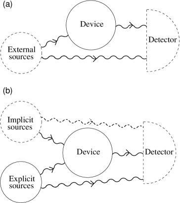
Figure 1: Schematics of eqs. (64) and (69). (a) In eq. (64), radiation of external sources is scattered by a device, and full radiation is measured by a detector. (b) In eq. (69), the sources are initially divided into implicit and explicit ones, and the detector is insensitive to the radiation of the implicit sources. To achieve full correspondence between the classical and quantum formulations, radiation of the implicit sources is added to the detected field by hand. Radiation of implicit sources which does ot does not reach the detector is shown schematically as a dashed wavy line, while all other types of radiation — as solid wavy lines. Devices drawn with dashed lines occur implicitly.

As a yardstick for quantum interactions, consider a classical scattering problem depicted in Fig. 1a. For simplicity we confine our discussion to the nonresonant field and current (the broad-band case). The general case will be restored in section V.2. In the arrangement in Fig. 1a, radiation of some external sources $A_{\mathrm{ext}}(x,t)$ is incident on a device. Full radiation $A_{\mathrm{tot}}(x,t)$ seen by a detector includes $A_{\mathrm{ext}}(x,t)$ and radiation of the device,

$${{\begin{aligned} A_{\mathrm{tot}}(x,t)=A_{\mathrm{ext}}(x,t)+\int dt^{\prime}\Delta_{\text{R}}(x,x^{\prime},t-t^{\prime})J(x^{\prime},t^{\prime}).\end{aligned}}}$$ (58)

The random current $J(x,t)$ describes the device. Sources of $A_{\mathrm{ext}}(x,t)$ and the detector occur implicitly; in Fig. 1a, they are drawn with dashed lines.

External radiation is by definition regular (nonstochastic). The only source of randomness is stochasticity of the current $J(x,t)$. Its most general characterisation is given by a conditional functional probability distribution,

$${{\begin{aligned} p\big{(}J\big{|}A_{\mathrm{ext}}\big{)}\geq 0.\end{aligned}}}$$ (59)

We stress that $p\big{(}J\big{|}A_{\mathrm{ext}}\big{)}$ is a functional of two c-number functions $J(x,t)$ and $A_{\mathrm{ext}}(x,t)$ and not a function of two scalar variables. An alternative characterisation of the device is given by the generating functional of stochastic averages of the random current conditional on the incident field,

$$\overline{\hskip 0.43057ptJ(x_{1},t_{1})\cdots J(x_{m},t_{m})\hskip 0.43057pt}\raisebox{-2.25002pt}{$|_{A_{\mathrm{ext}}}$}=\frac{\delta^{m}\Phi_{\mathrm{dev}}\big{(}\zeta\big{|}A_{\mathrm{ext}}\big{)}}{\delta\zeta(x_{1},t_{1})\cdots\delta\zeta(x_{m},t_{m})},$$

$$\Phi_{\mathrm{dev}}\big{(}\zeta\big{|}A_{\mathrm{ext}}\big{)}=\overline{\hskip 0.43057pt\exp\bigg{[}i\int dt\zeta(x,t)J(x,t)\bigg{]}\hskip 0.43057pt}\raisebox{-3.60004pt}{$\Big{|}_{A_{\mathrm{ext}}}$}.$$ (60)

For a general non-Markovian system, the conditional average $\overline{\hskip 0.43057pt\cdots\hskip 0.43057pt}\raisebox{-2.25002pt}{$|_{A_{\mathrm{ext}}}$}$ is written explicitly as a path integral,

$${{\begin{aligned} \Phi_{\mathrm{dev}}\big{(}\zeta\big{|}A_{\mathrm{ext}}\big{)}=\prod_{x,t}\bigg{\{}\int dJ(x,t)\bigg{\}}p\big{(}J\big{|}A_{\mathrm{ext}}\big{)}\exp\big{(}i\zeta J\big{)}.\end{aligned}}}$$ (61)

We again resort to condensed notation (30).

We do not introduce path integrals formally, thinking of them as multidimensional integrals in discretised time. This makes their algebraic manipulation straightforward. In particular, inverting the multidimensional Fourier-transformation (61) we find the formula,

$$\hskip 86.72267ptp\big{(}J\big{|}A_{\mathrm{ext}}\big{)}=\prod_{x,t}\bigg{\{}\frac{dtdx}{2\pi}\int d\zeta(x,t)\bigg{\}}\exp\big{(}-i\zeta J\big{)}\\ \times\Phi_{\mathrm{dev}}\big{(}\zeta\big{|}A_{\mathrm{ext}}\big{)},\hskip 86.72267pt$$ (62)

cf. eq. (114) in the appendix. The infinitesimal scaling factor $\Pi_{x,t}dxdt$ emphasises that our formulae are only symbolic. For more details see section VII and the appendix.

Full characterisation of the scattering experiment in Fig. 1a is given by the generating functional of joint stochatic averages of the field and current,

$$\hskip 86.72267pt\overline{\hskip 0.43057pt{\exp\big{(}i\eta A_{\mathrm{tot}}+i\zeta J\big{)}}\hskip 0.43057pt}\raisebox{-2.25002pt}{$|_{A_{\mathrm{ext}}}$}\\ =\overline{\hskip 0.43057pt\exp\big{[}i\eta\big{(}A_{\mathrm{ext}}+\Delta_{\text{R}}J\big{)}+i\zeta J\big{]}\hskip 0.43057pt}\raisebox{-2.25002pt}{$|_{A_{\mathrm{ext}}}$}.\hskip 86.72267pt$$ (63)

The RHS here may also be written explicitly as a functional integral,

$$\hskip 86.72267pt\overline{\hskip 0.43057pt{\exp\big{(}i\eta A_{\mathrm{tot}}+i\zeta J\big{)}}\hskip 0.43057pt}\raisebox{-2.25002pt}{$|_{A_{\mathrm{ext}}}$}=\prod_{x,t}\bigg{\{}\int dJ(x,t)\bigg{\}}p\big{(}J\big{|}A_{\mathrm{ext}}\big{)}\\ \times\exp\big{[}i\eta\big{(}A_{\mathrm{ext}}+\Delta_{\text{R}}J\big{)}+i\zeta J\big{]}.\hskip 86.72267pt$$ (64)

These formulae express two simple facts: that the full field is external field plus radiation of the device, cf. eq. (58), and that the sole source of stochasticity is randomness of $J(x,t)$.

IV.3 Quantum versus classical field-scattering problem

It is instructive to compare the classical eq. (63) to the quantum formula (57). Confining the latter for simplicity to the broad-band field and current we obtain,

$$\hskip 86.72267pt\Big{\langle}{\mathcal{T}}{\mbox{\rm\boldmath$:$}}\exp\big{(}i\eta{\hat{\mathcal{A}}}+i\zeta{\hat{\mathcal{J}}}\big{)}{\mbox{\rm\boldmath$:$}}\Big{\rangle}\\ =\Big{\langle}{\mathcal{T}}{\mbox{\rm\boldmath$:$}}\exp\big{[}i\eta\Delta_{\text{R}}\big{(}{\hat{\mathcal{J}}}+J_{\mathrm{e}}\big{)}+i\zeta{\hat{\mathcal{J}}}\big{]}{\mbox{\rm\boldmath$:$}}\Big{\rangle}.\hskip 86.72267pt$$ (65)

Reduced to the current modes, eq. (56) reads,

$${{\begin{aligned} \Phi_{\mathrm{dev}}\big{(}\zeta\big{|}A_{\mathrm{ext}}\big{)}=\Big{\langle}{\mathcal{T}}{\mbox{\rm\boldmath$:$}}\exp\big{(}i\zeta{\hat{\mathcal{J}}}\big{)}{\mbox{\rm\boldmath$:$}}\Big{\rangle}.\end{aligned}}}$$ (66)

We see that in quantum mechanics things are a trifle more complicated than in classical mechanics. While properties of the current operator depend on the full external field $A_{\mathrm{ext}}(x,t)$, those of the field operator depend on $A_{\mathrm{ext}}(x,t)$ through the current operator and separately on $J_{\mathrm{e}}(x,t)$ through the factor

$${{\begin{aligned} \exp\big{(}i\eta\Delta_{\text{R}}J_{\mathrm{e}}\big{)}\end{aligned}}}$$ (67)

in eq. (65). We therefore multiply eq. (65) by the additional factor,

$${{\begin{aligned} \exp\big{(}i\eta A_{\textrm{e}}\big{)}.\end{aligned}}}$$ (68)

The resulting quantum formula reads,

$$\hskip 86.72267pt\Big{\langle}{\mathcal{T}}{\mbox{\rm\boldmath$:$}}\exp\big{[}i\eta\big{(}{\hat{\mathcal{A}}}+A_{\textrm{e}}\big{)}+i\zeta{\hat{\mathcal{J}}}\big{]}{\mbox{\rm\boldmath$:$}}\Big{\rangle}\\ =\Big{\langle}{\mathcal{T}}{\mbox{\rm\boldmath$:$}}\exp\big{[}i\eta\big{(}A_{\textrm{ext}}+\Delta_{\text{R}}{\hat{\mathcal{J}}}\big{)}+i\zeta{\hat{\mathcal{J}}}\big{]}{\mbox{\rm\boldmath$:$}}\Big{\rangle},\hskip 86.72267pt$$ (69)

where use was made of the obvious relation,

$${{\begin{aligned} \exp\big{(}i\eta\Delta_{\text{R}}J_{\mathrm{e}}\big{)}\exp\big{(}i\eta A_{\textrm{e}}\big{)}=\exp\big{(}i\eta A_{\textrm{ext}}\big{)}.\end{aligned}}}$$ (70)

In eq. (69), the RHS and hence the LHS depend only on the full external field $A_{\mathrm{ext}}(x,t)$.

Comparing eq. (63) and (69) we see that they coincide up to the replacement of operators by c-numbers, and of the time-normal averages by classical stochastic averages,

$${{\begin{aligned} &{\hat{\mathcal{A}}}(x,t)+A_{\textrm{e}}(x,t)\leftrightarrow A_{\mathrm{tot}}(x,t),&&{\hat{\mathcal{J}}}(x,t)\leftrightarrow J(x,t),\\ &\langle{\mathcal{T}}{\mbox{\rm\boldmath$:$}}(\cdots){\mbox{\rm\boldmath$:$}}\rangle\leftrightarrow\overline{\hskip 0.43057pt(\cdots)\hskip 0.43057pt}.\end{aligned}}}$$ (71)

The field operator ${\hat{\mathcal{A}}}(x,t)$ thus corresponds not to the full field $A_{\mathrm{tot}}(x,t)$, but to the radiated field $A(x,t)$,

$$\hskip 86.72267ptA(x,t)=A_{\mathrm{tot}}(x,t)-A_{\mathrm{e}}(x,t)\\ =\int dt^{\prime}\Delta_{\text{R}}(x,x^{\prime},t-t^{\prime})\big{[}J(x^{\prime},t^{\prime})+J_{\mathrm{e}}(x^{\prime},t^{\prime})\big{]}.\hskip 86.72267pt$$ (72)

The latter is measured in the experimental arrangement shown in Fig. 1b. All external sources are divided into implicit and explicit ones. Implicit sources are responsible for the field $A_{\mathrm{e}}(x,t)$. This field affects the device but not the detector. Explicit sources are described by the current $J_{\mathrm{e}}(x,t)$. Radiation of the latter affects both the device and the detector.

That the detector sees radiation of some sources and does not see radiation of others may seem unnatural, but it reflects the situation in quantum mechanics where quantised fields and c-number sources are objects of different nature. In fact, whether the detector does or does not see $A_{\mathrm{e}}(x,t)$ is an additional assumption to be made in a detection model. We return to this question elsewhere.

IV.4 Cancellation of the in-field

The message of eq. (65) is that, under the time-normal averaging, classical radiation laws apply directly to Heisenberg operators. That is, in a time-normal average (and only in a time-normal average) we can write,

$$\hskip 86.72267pt{\hat{\mathcal{A}}}(x,t)=\int dx^{\prime}dt^{\prime}\Delta_{\text{R}}(x,x^{\prime},t-t^{\prime})\\ \times\big{[}{\hat{\mathcal{J}}}(x^{\prime},t^{\prime})+J_{\textrm{e}}(x^{\prime},t^{\prime})\big{]}.\hskip 86.72267pt$$ (73)

It is instructive to compare this relation to the standard quantum-field-theoretical formula connecting the Heisenberg and free-field operators. Without the source, (73) becomes,

$${{\begin{aligned} {\hat{\mathcal{A}}}(x,t)&=\int dx^{\prime}dt^{\prime}\Delta_{\text{R}}(x,x^{\prime},t-t^{\prime}){\hat{\mathcal{J}}}(x^{\prime},t^{\prime}).\end{aligned}}}$$ (74)

As a Hilbert-space formula, this relation cannot be correct because it does not preserve commutational relations. The right formula Schweber (2005) should include the free-field operator (in-field),

$$\hskip 86.72267pt{\hat{\mathcal{A}}}(x,t)=\hat{A}(x,t)\\ \ \ \ +\int dx^{\prime}dt^{\prime}\Delta_{\text{R}}(x,x^{\prime},t-t^{\prime}){\hat{\mathcal{J}}}(x^{\prime},t^{\prime}).\hskip 86.72267pt$$ (75)

Under the time-normal averaging, the in-field cancels. This is partly due to the vacuum initial state of the field, but only partly. The in-field operator $\hat{A}(x,t)$ does not commute with ${\hat{\mathcal{A}}}(x,t)$ and ${\hat{\mathcal{J}}}(x,t)$, so that its disappearance under the time-normal averaging in eq. (65) is anything but trivial.

V Conditional P-functional

V.1 Conditional time-normal quasiprobability distribution of the quantum current

In conventional phase-space approaches Wolf and Mandel (1995); Agarwal and Wolf (1970), each type of operator ordering is associated with a corresponding type of quasidistribution. Formally, quasidistributions may be defined postulating that the relation between quantum averages of operators ordered in a particular way and the associated quasidistribution emulates the classical relation between stochastic averages and probability distributions. Applying this idea to interacting systems, it is natural to introduce conditional functional time-normal quasiprobability distributions, or conditional P-functionals, of quantum dynamical variables. By definition, they are related to time-normal averages of these variables by formulae emulating classical relations between multitime stochastic averages and corresponding functional probability distributions. Conditional P-functionals thus generalise two concepts: that of conditional functional probability distribution to quantum mechanics, and that of P-function to Heisenberg fields.

So, postulating eq. (62) for the quantum $\Phi_{\mathrm{dev}}$ given by (66), we define the conditional P-functional of the quantum current as,

$$\hskip 86.72267ptp\big{(}J\big{|}A_{\mathrm{ext}}\big{)}=\prod_{t}\bigg{\{}\frac{dtdx}{2\pi}\int d\zeta(t)\bigg{\}}\\ \times\bigg{\langle}{\mathcal{T}}{\mbox{\rm\boldmath$:$}}\exp\bigg{\{}i\int dxdt\zeta(x,t)\big{[}{\hat{\mathcal{J}}}(x,t)-J(x,t)\big{]}\bigg{\}}{\mbox{\rm\boldmath$:$}}\bigg{\rangle}.\hskip 86.72267pt$$ (76)

The inverse relation emulates eq. (61):

$${{\begin{aligned} \bigg{\langle}{\mathcal{T}}{\mbox{\rm\boldmath$:$}}\exp\bigg{[}i\int dt\zeta(x,t){\hat{\mathcal{J}}}(x,t)\bigg{]}{\mbox{\rm\boldmath$:$}}\bigg{\rangle}=\prod_{x,t}\bigg{\{}\int dJ(x,t)\bigg{\}}p\big{(}J\big{|}A_{\mathrm{ext}}\big{)}\exp\bigg{[}i\int dxdt\zeta(x,t)J(x,t)\bigg{]}.\end{aligned}}}$$ (77)

Note that the logic here is the other way around compared to eqs. (61), (62). The primary quantity is functional (66), $p\big{(}J\big{|}A_{\mathrm{ext}}\big{)}$ is defined by eq. (76), while eq. (77) is found inverting the latter.

Using eq. (77), eq. (57) may be written in the form,

$$\bigg{\langle}{\mathcal{T}}{\mbox{\rm\boldmath$:$}}\exp\bigg{(}i\int dxdt\Big{\{}\eta(x,t)\big{[}{\hat{\mathcal{A}}}(x,t)+A_{\mathrm{e}}(x,t)\big{]}+\zeta(x,t){\hat{\mathcal{J}}}(x,t)\Big{\}}\bigg{)}{\mbox{\rm\boldmath$:$}}\bigg{\rangle}\\ =\prod_{x,t}\bigg{\{}\int dJ(x,t)\bigg{\}}p\big{(}J\big{|}A_{\mathrm{ext}}\big{)}\exp\bigg{(}i\int dxdt\bigg{\{}\zeta(x,t)J(x,t)\\ +\eta(x,t)\bigg{[}A_{\mathrm{ext}}(x,t)+\int dx^{\prime}dt^{\prime}\Delta_{\text{R}}(t-t^{\prime})J(x^{\prime},t^{\prime})\bigg{]}\bigg{\}}\bigg{)}.$$ (78)

This is a quantum analog of eq. (64). It differs from the latter in replacements (71), and in that the P-functional $p\big{(}J\big{|}A_{\mathrm{ext}}\big{)}$ needs not be nonnegative.

Reality and causality properties of the P-functionals are inherited from those of the the time-normal averages (cf. section II.4). Using reality of the latter it is straightforward to show that the P-functionals are also real. We avoid formulating causality conditions for the P-functionals which are not transparent. It suffices to say that causality properties of the P-functionals coincide with those of the functional probability distributions.

Equation (78) may be extended to a full quantum treatment replacing,

$${{\begin{aligned} A_{\mathrm{e}}(x,t)\to A_{\mathrm{e}}(x,t)+a_{\mathrm{e}}(x,t).\end{aligned}}}$$ (79)

In classical mechanics, $a_{\mathrm{e}}(x,t)$ does not exist. It appears only in quantum mechanics, where it reflects noncommutativity of the operators. $a_{\mathrm{e}}(x,t)$ and $A_{\mathrm{e}}(x,t)$ not just differ, but are of different nature: one is an auxiliary variable, and the other is an external source. It is a nontrivial property of quantum dynamics that they occur in the functional $\Phi$ as a sum. All quantum-classical correspondences we discuss in this paper are subject to two facts: absence of Planck’s constant in dynamical relations in causal variables, and the consistency relation (39). In no way should importance of the latter be overlooked.

V.2 Extension to the general case

The main advantage of conditional P-functionals is that they allow for doing quantum electrodynamics by thinking classically. As an example, let us “derive” eq. (57) from classical considerations and correspondence rules (71). In the general case of Hamiltonian (23), eqs. (71) should be supplemented by correspondences for dipoles and optical fields,

$${{\begin{aligned} {\hat{\mathcal{E}}}(x,t)&\leftrightarrow E(x,t),&{\hat{\mathcal{D}}}(x,t)&\leftrightarrow D(x,t),&{\hat{\mathcal{E}}}^{{\dagger}}(x,t)&\leftrightarrow E^{*}(x,t),&{\hat{\mathcal{D}}}^{{\dagger}}(x,t)&\leftrightarrow D^{*}(x,t),\end{aligned}}}$$ (80)

where $E(x,t)$ is the radiated optical field,

$${{\begin{aligned} E(x,t)=\int dx^{\prime}dt^{\prime}G_{\text{R}}(x,x^{\prime},t-t^{\prime})\big{[}D(x,t)+D_{\textrm{e}}(x,t)\big{]}.\end{aligned}}}$$ (81)

The device is now formally described by two random quantities, current $J(x,t)$ and dipole $D(x,t)$. Their joint probablity distribution is conditional on the external fields (48),

$${{\begin{aligned} p\big{(}J,D,D^{*}\big{|}A_{\text{ext}},E_{\text{ext}},E_{\text{ext}}^{*}\big{)}\geq 0.\end{aligned}}}$$ (82)

Using it we can construct the characteristic functional of joint statistical averages of the currents and dipoles,

$$\overline{\hskip 0.43057pt\exp\big{(}i\zeta J+i\nu^{*}D-i\nu D^{*}\big{)}\hskip 0.43057pt}=\prod_{x,t}\bigg{\{}\int dJ(x,t)d^{2}D(x,t)\bigg{\}}\\ \times p\big{(}J,D,D^{*}\big{|}A_{\text{ext}},E_{\text{ext}},E_{\text{ext}}^{*}\big{)}\exp\big{(}i\zeta J+i\nu^{*}D-i\nu D^{*}\big{)}.$$ (83)

Using eqs. (72) and (81), we also obtain the characteristic functional of joint statistical averages of the fields, currents and dipoles,

$$\overline{\hskip 0.43057pt\exp\big{(}i\eta A+i\mu^{*}E-i\mu E^{*}+i\zeta J+i\nu^{*}D-i\nu D^{*}\big{)}\hskip 0.43057pt}\\ =\prod_{x,t}\bigg{\{}\int dJ(x,t)d^{2}D(x,t)\bigg{\}}p\big{(}J,D,D^{*}\big{|}A_{\text{ext}},E_{\text{ext}},E_{\text{ext}}^{*}\big{)}\\ \times\exp\big{[}i\eta\Delta_{\text{R}}\big{(}J+J_{\textrm{e}}\big{)}+i\mu^{*}G_{\text{R}}\big{(}D+D_{\textrm{e}}\big{)}-i\mu G_{\text{R}}^{*}\big{(}D^{*}+D_{\textrm{e}}^{*}\big{)}+i\zeta J+i\nu^{*}D-i\nu D^{*}\big{]}.$$ (84)

Comparing these two relations, we find the formula,

$$\overline{\hskip 0.43057pt\exp\big{(}i\eta A+i\mu^{*}E-i\mu E^{*}+i\zeta J+i\nu^{*}D-i\nu D^{*}\big{)}\hskip 0.43057pt}\\ =\overline{\hskip 0.43057pt\exp\big{[}i\eta\Delta_{\text{R}}\big{(}J+J_{\textrm{e}}\big{)}+i\mu^{*}G_{\text{R}}\big{(}D+D_{\textrm{e}}\big{)}-i\mu G_{\text{R}}^{*}\big{(}D^{*}+D_{\textrm{e}}^{*}\big{)}+i\zeta J+i\nu^{*}D-i\nu D^{*}\big{]}\hskip 0.43057pt}.$$ (85)

Applying replacements (71), (80) to this relation we indeed recover eq. (57).

Consider now the logic of this “derivation” in more detail. Applying the said replacements to eq. (83) is equivalent to defining the conditional P-functional,

$$p\big{(}J,D,D^{*}\big{|}A_{\text{ext}},E_{\text{ext}},E_{\text{ext}}^{*}\big{)}=\prod_{x,t}\bigg{\{}\frac{(dtdx)^{3}}{2\pi^{3}}\int d\zeta(x,t)d^{2}\nu(x,t)\bigg{\}}\\ \times\Big{\langle}{\mathcal{T}}{\mbox{\rm\boldmath$:$}}\exp\big{[}i\zeta\big{(}{\hat{\mathcal{J}}}-J\big{)}+i\nu^{*}\big{(}{\hat{\mathcal{D}}}-D\big{)}-i\nu\big{(}{\hat{\mathcal{D}}}^{{\dagger}}-D^{*}\big{)}\big{]}{\mbox{\rm\boldmath$:$}}\Big{\rangle}.$$ (86)

Inverting this definition we find the quantum counterpart of (83),

$$\Big{\langle}{\mathcal{T}}{\mbox{\rm\boldmath$:$}}\exp\big{(}i\zeta{\hat{\mathcal{J}}}+i\nu^{*}{\hat{\mathcal{D}}}-i\nu{\hat{\mathcal{D}}}^{{\dagger}}\big{)}{\mbox{\rm\boldmath$:$}}\Big{\rangle}=\prod_{x,t}\bigg{\{}\int dJ(x,t)d^{2}D(x,t)\bigg{\}}\\ \times p\big{(}J,D,D^{*}\big{|}A_{\text{ext}},E_{\text{ext}},E_{\text{ext}}^{*}\big{)}\exp\big{(}i\zeta J+i\nu^{*}D-i\nu D^{*}\big{)}.$$ (87)

Furthermore, applying the quantum-classical correspondences to eq. (84) we obtain,

$$\Big{\langle}{\mathcal{T}}{\mbox{\rm\boldmath$:$}}\exp\big{(}i\eta{\hat{\mathcal{A}}}+i\mu^{*}{\hat{\mathcal{E}}}-i\mu{\hat{\mathcal{E}}}^{{\dagger}}+i\zeta{\hat{\mathcal{J}}}+i\nu^{*}{\hat{\mathcal{D}}}-i\nu{\hat{\mathcal{D}}}^{{\dagger}}\big{)}{\mbox{\rm\boldmath$:$}}\Big{\rangle}\\ =\prod_{x,t}\bigg{\{}\int dJ(x,t)d^{2}D(x,t)\bigg{\}}p\big{(}J,D,D^{*}\big{|}A_{\text{ext}},E_{\text{ext}},E_{\text{ext}}^{*}\big{)}\\ \times\exp\big{[}i\eta\Delta_{\text{R}}\big{(}J+J_{\textrm{e}}\big{)}+i\mu^{*}G_{\text{R}}\big{(}D+D_{\textrm{e}}\big{)}-i\mu G_{\text{R}}^{*}\big{(}D^{*}+D_{\textrm{e}}^{*}\big{)}+i\zeta J+i\nu^{*}D-i\nu D^{*}\big{]}.$$ (88)

Comparing eqs. (87) and (88) we recover eq. (57). However, there is no other way to actually prove (88) except by showing that it follows from (57), which in turn is another form of (45). Strictly speaking, eq. (88) is eq. (45) written using notation (54), (56) and definition (86). One may say that eq. (88) is a mnemonic form of the quantum relation (45): classical connotations of the former allow one to easily memorise it. The actual derivation of eqs. (45), (57) and (88) is that given in Refs. Plimak and Stenholm (2011b, a). All we do here is rewrite the obscure eq. (45) in a series of physically more transparent forms.

VI Self-action problem in terms of P-functionals

Conditional P-functionals also give a natural description of the electromagnetic self-action, or “dressing,” problem. Again, we start from a more compact broad-band case. Reduced to fields and currents, the dressing relation (49) becomes,

$${{\begin{aligned} \Phi_{\mathrm{dev}}\big{(}\zeta\big{|}A_{\text{ext}}\big{)}=\exp\bigg{(}-i\frac{\delta}{\delta A_{\mathrm{ext}}}\Delta_{\text{R}}\frac{\delta}{\delta\zeta}\bigg{)}\Phi_{\mathrm{dev}}^{\mathrm{I}}\big{(}\zeta\big{|}A_{\text{ext}}\big{)},\end{aligned}}}$$ (89)

This formula implies the response definition of $\Phi_{\mathrm{dev}}^{\mathrm{I}}$ by eq. (51). Following the pattern of eqs. (76), (77) we define,

$$\hskip 86.72267ptp\big{(}J\big{|}A_{\mathrm{ext}}\big{)}=\prod_{x,t}\bigg{\{}\frac{dxdt}{2\pi}\int d\zeta(x,t)\bigg{\}}\\ \times\text{Tr}\hat{\rho}_{\textrm{dev}}{{\mathcal{T}}{\mbox{\rm\boldmath$:$}}\exp\big{[}i\zeta\big{(}\hat{J}^{\prime}-J\big{)}\big{]}{\mbox{\rm\boldmath$:$}}},\hskip 86.72267pt$$ (90)

and

$$\hskip 86.72267pt\Phi_{\mathrm{dev}}^{\mathrm{I}}\big{(}\zeta\big{|}A_{\text{ext}}\big{)}=\text{Tr}\hat{\rho}_{\textrm{dev}}{\mathcal{T}}{\mbox{\rm\boldmath$:$}}\exp\big{(}i\zeta\hat{J}^{\prime}\big{)}{\mbox{\rm\boldmath$:$}}\\ =\prod_{x,t}\bigg{\{}\int dJ(x,t)\bigg{\}}p^{\mathrm{I}}\big{(}J\big{|}A_{\mathrm{ext}}\big{)}\exp\big{(}i\zeta J\big{)}.\hskip 86.72267pt$$ (91)

$\hat{J}^{\prime}(x,t)$ was defined in section III.6. We use condensed notation (30). The meaning of $p^{\mathrm{I}}$ is yet to be understood. Substituting (91) into the dressing formula (89) we have,

$$\hskip 86.72267pt\Phi_{\mathrm{dev}}\big{(}\zeta\big{|}A_{\mathrm{ext}}\big{)}=\prod_{x,t}\bigg{\{}\int dJ(x,t)\bigg{\}}\\ \times\exp\bigg{(}-i\frac{\delta}{\delta A_{\mathrm{ext}}}\Delta_{\text{R}}\frac{\delta}{\delta\zeta}\bigg{)}p^{\mathrm{I}}\big{(}J\big{|}A_{\mathrm{ext}}\big{)}\exp\big{(}i\zeta J\big{)}.\hskip 86.72267pt$$ (92)

The integrand here is transformed in two steps:

$$\hskip 86.72267pt\exp\bigg{(}-i\frac{\delta}{\delta A_{\mathrm{ext}}}\Delta_{\text{R}}\frac{\delta}{\delta\zeta}\bigg{)}p^{\mathrm{I}}\big{(}J\big{|}A_{\mathrm{ext}}\big{)}\exp\big{(}i\zeta J\big{)}\\ =\exp\big{(}i\zeta J\big{)}\exp\bigg{(}\frac{\delta}{\delta A_{\mathrm{ext}}}\Delta_{\text{R}}J\bigg{)}p^{\mathrm{I}}\big{(}J\big{|}A_{\mathrm{ext}}\big{)}\\ =\exp\big{(}i\zeta J\big{)}p^{\mathrm{I}}\big{(}J\big{|}A_{\mathrm{ext}}+\Delta_{\text{R}}J\big{)}.\hskip 86.72267pt$$ (93)

We use condensed notation (33). The first step in (93) is trivial; the second one is an application of a functional shift operator. This way,

$$\hskip 86.72267pt\Phi_{\mathrm{dev}}\big{(}\zeta\big{|}A_{\mathrm{ext}}\big{)}=\prod_{x,t}\bigg{\{}\int dJ(x,t)\bigg{\}}\\ \times p^{\mathrm{I}}\big{(}J\big{|}A_{\mathrm{ext}}+\Delta_{\text{R}}J\big{)}\exp\big{(}i\zeta J\big{)},\hskip 86.72267pt$$ (94)

and

$${{\begin{aligned} p\big{(}J\big{|}A_{\mathrm{ext}}\big{)}=p^{\mathrm{I}}\big{(}J\big{|}A_{\mathrm{ext}}+\Delta_{\text{R}}J\big{)}.\end{aligned}}}$$ (95)

The classical content of this relation is crystal clear. Functional $p\big{(}J\big{|}A_{\mathrm{ext}}\big{)}$ describes statistical properties of the current $J(x,t)$ conditional on the external (macroscopic) field $A_{\mathrm{ext}}(x,t)$. Functional $p^{\mathrm{I}}\big{(}J\big{|}A_{\mathrm{loc}}\big{)}$ describes statistical properties of the current $J(x,t)$ conditional on the local (microscopic) field $A_{\mathrm{loc}}(x,t)$. The latter equals $A_{\mathrm{ext}}(t)$ plus self-radiation of the current,

$$\hskip 86.72267ptA_{\mathrm{loc}}(x,t)=A_{\mathrm{ext}}(x,t)\\ +\int dx^{\prime}dt^{\prime}\Delta_{\text{R}}(x,x^{\prime},t-t^{\prime})J(x^{\prime},t^{\prime}).\hskip 86.72267pt$$ (96)

In quantum electrodynamics, this interpretation applies with replacement of “statistical” by “quasistatistical.”

In the general case, the dressing relation for P-functionals reads,

$$\hskip 86.72267ptp\big{(}J,D,D^{*}\big{|}A_{\mathrm{ext}},E_{\mathrm{ext}},E_{\mathrm{ext}}^{*}\big{)}\\ =p^{\mathrm{I}}\big{(}J,D,D^{*}\big{|}A_{\mathrm{ext}}+\Delta_{\text{R}}J,E_{\mathrm{ext}}+G_{\text{R}}D,E_{\mathrm{ext}}^{*}+G_{\text{R}}^{*}D^{*}\big{)},\hskip 86.72267pt$$ (97)

where the functional $p_{\text{I}}\big{(}J,D,D^{*}\big{|}A_{\mathrm{ext}},E_{\mathrm{ext}},E_{\mathrm{ext}}^{*}\big{)}$ is given by the relation,

$$\hskip 86.72267ptp^{\mathrm{I}}\big{(}J,D,D^{*}\big{|}A_{\mathrm{ext}},E_{\mathrm{ext}},E_{\mathrm{ext}}^{*}\big{)}\\ =\prod_{x,t}\bigg{\{}\frac{(dxdt)^{3}}{2\pi^{3}}\int d\zeta(x,t)d^{2}\nu(x,t)\bigg{\}}\text{Tr}\hat{\rho}_{\textrm{dev}}\\ \times{\mathcal{T}}{\mbox{\rm\boldmath$:$}}\exp\big{[}i\zeta\big{(}\hat{J}^{\prime}-J\big{)}-i\mu^{*}\big{(}\hat{D}^{\prime}-D\big{)}+i\mu\big{(}\hat{D}^{\prime{\dagger}}-D^{*}\big{)}\big{]}{\mbox{\rm\boldmath$:$}}.\hskip 86.72267pt$$ (98)

The primed operators were defined in section III.6. Derivation and interpretation of eq. (97) are no different from those of eq. (95).

VII Discussion: causality and regularisations

It should not be overlooked that eq. (95) is consistent only due to causality properties of P-functionals. Here is a simple example. Assume that all quantities in (95) do not depend on time. The external field shifts the Gaussian distribution of the current,

$${{\begin{aligned} p^{\mathrm{I}}\big{(}J\big{|}A_{\mathrm{e}}\big{)}=\frac{1}{\sqrt{2\pi}\,J_{0}}\exp\bigg{[}-\frac{\big{(}J-\chi A_{\mathrm{e}}\big{)}^{2}}{2J_{0}^{2}}\bigg{]},\end{aligned}}}$$ (99)

where $J_{0}>0$ and $\chi$ are real constants. In place of (96) we postulate a scalar formula,

$${{\begin{aligned} A_{\mathrm{loc}}=A_{\mathrm{e}}+\Delta_{\text{R}}J,\end{aligned}}}$$ (100)

where $\Delta_{\text{R}}$ is one more real constant. For the “dressed current” we find,

$${{\begin{aligned} p\big{(}J\big{|}A_{\mathrm{e}}\big{)}=\frac{1}{\sqrt{2\pi}\,J_{0}}\exp\bigg{[}-\frac{\big{(}J-\chi\Delta_{\text{R}}J-\chi A_{\mathrm{e}}\big{)}^{2}}{2J_{0}^{2}}\bigg{]}.\end{aligned}}}$$ (101)

This function is not normalised,

$${{\begin{aligned} \int dJ\,p\big{(}J\big{|}A_{\mathrm{e}}\big{)}=\frac{1}{1-\chi\Delta_{\text{R}}}\neq 1,\end{aligned}}}$$ (102)

and cannot be a probability distribution for anything.

To see how causality breaks this vicious circle of same-time interactions consider another simple example. We generalise (99) to two currents,

$$\hskip 86.72267ptp^{\mathrm{I}}\big{(}J,J^{\prime}\big{|}A_{\mathrm{e}},A_{\mathrm{e}}^{\prime}\big{)}\\ =\frac{1}{2\pi J_{0}^{2}}\exp\bigg{[}-\frac{\big{(}J-\chi A_{\mathrm{e}}\big{)}^{2}+\big{(}J^{\prime}-\chi A_{\mathrm{e}}^{\prime}\big{)}^{2}}{2J_{0}^{2}}\bigg{]}.\hskip 86.72267pt$$ (103)

The primed current preceeds the unprimed one in time; therefore it may affect the latter but not vice versa. Same-time interactions are not allowed either. The simplest case of such interaction is,

$${{\begin{aligned} &A_{\mathrm{loc}}=A_{\mathrm{e}}+\Delta_{\text{R}}J^{\prime},&&A_{\mathrm{loc}}^{\prime}=A_{\mathrm{e}}^{\prime}.\end{aligned}}}$$ (104)

For the dressed currents we then have,

$$\hskip 86.72267ptp\big{(}J,J^{\prime}\big{|}A_{\mathrm{e}},A_{\mathrm{e}}^{\prime}\big{)}=\frac{1}{2\pi J_{0}^{2}}\\ \times\exp\bigg{[}-\frac{\big{(}J-\chi\Delta_{\text{R}}J^{\prime}-\chi A_{\mathrm{e}}\big{)}^{2}+\big{(}J^{\prime}-\chi A_{\mathrm{e}}^{\prime}\big{)}^{2}}{2J_{0}^{2}}\bigg{]}.\hskip 86.72267pt$$ (105)

Unlike (101), this function is both positive and normalised,

$${{\begin{aligned} \int dJ^{\prime}\int dJ\,p\big{(}J,J^{\prime}\big{|}A_{\mathrm{e}},A_{\mathrm{e}}^{\prime}\big{)}=1.\end{aligned}}}$$ (106)

It is therefore a genuine two-dimensional conditional probability distribution for a correlated pair of currents.

The order of integrations in (106) is chosen so as to make the result obvious. Indeed, (105) has the structure,

$${{\begin{aligned} p\big{(}J,J^{\prime}\big{|}A_{\mathrm{e}},A_{\mathrm{e}}^{\prime}\big{)}=p\big{(}J\big{|}A_{\mathrm{e}},J^{\prime}\big{)}p^{\prime}\big{(}J^{\prime}\big{|}A_{\mathrm{e}}^{\prime}\big{)},\end{aligned}}}$$ (107)

where

$${{\begin{aligned} p\big{(}J\big{|}A_{\mathrm{e}},J^{\prime}\big{)}&=\frac{1}{\sqrt{2\pi}\,J_{0}}\exp\bigg{[}-\frac{\big{(}J-\chi\Delta_{\text{R}}J^{\prime}-\chi A_{\mathrm{e}}\big{)}^{2}}{2J_{0}^{2}}\bigg{]},\\ p^{\prime}\big{(}J^{\prime}\big{|}A_{\mathrm{e}}^{\prime}\big{)}&=\frac{1}{\sqrt{2\pi}\,J_{0}}\exp\bigg{[}-\frac{\big{(}J^{\prime}-\chi A_{\mathrm{e}}^{\prime}\big{)}^{2}}{2J_{0}^{2}}\bigg{]}.\end{aligned}}}$$ (108)

The later current is conditional on the earlier one and the external field. The earlier current is conditional only on the external field. Similar structures should emerge for any time sequence of currents irrespective of any detals of the interaction. The only requirement is that each current depends only on those preceding it in time.

In real problems with continuous time, critical for cancellation of same-time interactions are regularisations. So, in Ref. Plimak et al. (2003), causal regularisation was applied to the retarded Green function of the emerging equation for phase-space amplitudes. This made noise sources present in the said equation independent of the amplitudes at the same time, resulting in the Ito calculus being chosen. The effect of causal regularisation is thus twofold: to introduce an infinitesimal delay into the phase-space equation, which is in essence time discretisation, and to prevent same-time interactions. A conceptual connection between the above simple examples and the causal regularisation is obvious. For a discussion of the connection between causal regularisation and suppression of infinities in relativistic quantum field theory we refer the reader to appendix D of Ref. Plimak and Stenholm (2011b).

VIII Conclusion and outlook

It is shown that phase-space concepts such as time-normal operator ordering and P-functonal provide a natural framework for quantum interactions of light and matter. In a forthcoming paper Plimak and Stenholm (2011d) this framework will be extended to macroscopic interactions of distinguishable devices.

IX Acknowledgements

Support of SFB/TRR 21 and of the Humboldt Foundation is gratefully acknowledged.

*

Appendix A Functional probability distributions and inversion formulae

The goal of this appendix is to derive the inversion formula (62), and to point to mathematical complications hidden behind apparent simplicity of our formulae. For simplicity we consider a c-number random quantity $J(t)$. For general non-Markovian systems, classical statistical averaging is formally a functional (path) integral,

$${{\begin{aligned} \overline{\hskip 0.43057ptJ(t_{1})\cdots J(t_{m})\hskip 0.43057pt}=\prod_{t}\bigg{\{}\int dJ(t)\bigg{\}}\,p(J)\,J(t_{1})\cdots J(t_{m}),\end{aligned}}}$$ (109)

where $p(J)$ is a functional probability distribution over the random functions (paths) $J(t)$. We emphasise that $p(J)$ is not a function of variable $J$, but a functional of a function $J(t)$.

For all practical purposes, $t$ in (109) may be thought of as a discrete index. Functional integration is then regarded a multiple integration over variables $J(t)=J_{t}$, each defined in an infinitely narrow Trotter time slice $\Delta t$ labelled by index $t$. With this simplified view, algebraic manipulation of the path integral becomes straightforward. For example, let us express $p(J)$ in terms of the characteritic functional of quantum averages (109),

$$\hskip 86.72267pt\Phi\big{(}\zeta\big{)}=\overline{\hskip 0.43057pt\exp\bigg{[}i\int dt\zeta(t)J(t)\bigg{]}\hskip 0.43057pt}\\ =\prod_{t}\bigg{\{}\int dJ(t)\bigg{\}}p(J)\exp\bigg{[}i\int dt\zeta(t)J(t)\bigg{]}.\hskip 86.72267pt$$ (110)

Thinking discretised time we replace,

$${{\begin{aligned} \exp\bigg{[}i\int dt\zeta(t)J(t)\bigg{]}\to\prod_{t}\mathrm{e}^{i\Delta t\zeta_{t}J_{t}}.\end{aligned}}}$$ (111)

The discretised approximation to (110) reads,

$${{\begin{aligned} \Phi\big{(}\zeta\big{)}=\prod_{t}\bigg{\{}\int\mathrm{e}^{i\Delta t\zeta_{t}J_{t}}dJ_{t}\bigg{\}}\,p(J).\end{aligned}}}$$ (112)

This is nothing but a multidimensional Fourier-transform. Inverting it “slicewise” we find,

$$\hskip 86.72267ptp(J)=\prod_{t}\bigg{\{}\frac{\Delta t}{2\pi}\int\mathrm{e}^{-i\Delta t\zeta_{t}J_{t}}d\zeta_{t}\bigg{\}}\Phi\big{(}\zeta\big{)}\\ =\prod_{t}\bigg{\{}\frac{\Delta t}{2\pi}\int d\zeta_{t}\bigg{\}}\Phi\big{(}\zeta\big{)}\exp\Big{[}-i\Delta t\sum_{t}\zeta_{t}J_{t}\Big{]}.\hskip 86.72267pt$$ (113)

Restoring continuity of time, we obtain the inversion formula,

$${{\begin{aligned} p(J)=\prod_{t}\bigg{\{}\frac{dt}{2\pi}\int d\zeta(t)\bigg{\}}\exp\bigg{[}-i\int dt\zeta(t)J(t)\bigg{]}\Phi\big{(}\zeta\big{)}.\end{aligned}}}$$ (114)

The infinitesimal factor $\prod_{t}dt$ leaves no doubt that this expression is only symbolic.

It should be noted that the notation we use for path integrals is equally symbolic. As an example, consider a well defined mathematical concept: the Wiener process. In discretised time, the probability density for the Wiener process reads,

$${{\begin{aligned} \prod_{t}\bigg{\{}\frac{d\Delta J_{t}}{\sqrt{2\pi\Delta t}}\exp\bigg{[}-\frac{\big{(}\Delta J_{t}\big{)}^{2}}{2\Delta t}\bigg{]}\bigg{\}},\end{aligned}}}$$ (115)

where $\Delta J_{t}=J_{t}-J_{t-\Delta t}$ are stochastic increments. From the first glance, continuous limit may be achieved introducing the discretised derivative,

$${{\begin{aligned} J^{\prime}_{t}=\frac{\Delta J_{t}}{\Delta t}.\end{aligned}}}$$ (116)

so that

$$\hskip 86.72267pt\prod_{t}\bigg{\{}\frac{d\Delta J_{t}}{\sqrt{2\pi\Delta t}}\exp\bigg{[}-\frac{\big{(}\Delta J_{t}\big{)}^{2}}{2\Delta t}\bigg{]}\bigg{\}}\\ =\prod_{t}\bigg{[}dJ^{\prime}_{t}\sqrt{\frac{\Delta t}{2\pi}}\bigg{]}\exp\bigg{[}-\sum_{t}\frac{\Delta t\big{(}J^{\prime}_{t}\big{)}^{2}}{2}\bigg{]}.\hskip 86.72267pt$$ (117)

In the continuous limit, we have for the probability density,

$${{\begin{aligned} \prod_{t}\bigg{[}dJ^{\prime}(t)\sqrt{\frac{dt}{2\pi}}\bigg{]}\exp\bigg{\{}-\frac{1}{2}\int dt\big{[}J^{\prime}(t)\big{]}^{2}\bigg{\}}.\end{aligned}}}$$ (118)

Infinitesimal scaling factors are indeed eliminated from the exponent, but the overall factor $\prod_{t}\sqrt{dt}$ persists. Because of this factor, quantity (118) is zero for all functions for which the integral in the exponent is defined (as expected). For nondifferentiable functions — which are of actual interest — eq. (118) is useless, because anyway it has to be specified through some limiting procedure. Hence (118) is no more than a symbolic way of writing the discretised approximation (115).

References

- Plimak et al. (2015) L. I. Plimak, M. Ivanov, A. Aiello, and S. Stenholm, Phys. Rev. A (2015).
- Wolf and Mandel (1995) E. Wolf and L. Mandel, Optical Coherence and Quantum Optics (Cambridge University Press, Cambridge, 1995).
- Agarwal and Wolf (1970) G. S. Agarwal and E. Wolf, Phys. Rev. D 2, 2161 (1970).
- Plimak and Stenholm (2011a) L. I. Plimak and S. Stenholm, arXive:1104.3809v2 (2011a).
- Schrödinger (1926) E. Schrödinger, Die Naturwissenschaften 14, 664 (1926).
- Feynman (1948) R. P. Feynman, Rev. Mod. Phys. 20, 367 (1948), the observation we refer to is in footnote 15 on page 375.
- Glauber (1963) R. J. Glauber, Phys. Rev. 130, 2529 (1963).
- Kelley and Kleiner (1964) P. L. Kelley and W. H. Kleiner, Phys. Rev. 136, A316 (1964).
- Glauber (1965) R. J. Glauber, Quantum Optics and Electronics. In Les Houches Summer School of Theoretical Physics (Gordon and Breach, New York, 1965).
- de Haan (1985) M. de Haan, Physica 132A, 375, 397 (1985).
- Bykov and Tatarskii (1989) V. P. Bykov and V. I. Tatarskii, Phys. Lett. A 136, 77 (1989).
- Tatarskii (1990) V. I. Tatarskii, Phys. Lett. A 144, 491 (1990).
- Plimak and Stenholm (2008a) L. I. Plimak and S. Stenholm, Ann. Phys. (N.Y.) 323, 1963 (2008a).
- Plimak and Stenholm (2008b) L. I. Plimak and S. Stenholm, Ann. Phys. (N.Y.) 323, 1989 (2008b).
- Plimak and Stenholm (2009) L. I. Plimak and S. Stenholm, Ann. Phys. (N.Y.) 324, 600 (2009).
- Plimak and Stenholm (2011b) L. I. Plimak and S. Stenholm, Phys. Rev. D 84, 065025 (2011b).
- Belinicher and Tikhodeev (1988) V. I. Belinicher and S. G. Tikhodeev, Soviet Physics Doklady 33, 516 (1988).
- Plimak (1994) L. I. Plimak, Phys. Rev. A 50, 2120 (1994).
- Plimak et al. (2003) L. I. Plimak, M. Fleischhauer, M. K. Olsen, and M. J. Collett, Phys. Rev. A 67, 013812 (2003).
- Schweber (2005) S. Schweber, An Introduction to Relativistic Quantum Field Theory (Dover, 2005).
- Schwinger (1961) J. S. Schwinger, J. Math. Phys. 2, 407 (1961).
- Konstantinov and Perel (1960) O. V. Konstantinov and V. I. Perel, Zh. Eksp. Theor. Phys. 39, 197 (1960), [Sov. Phys. JETP 12, 142 (1961)].
- Keldysh (1964) L. V. Keldysh, Zh. Eksp. Theor. Phys. 47, 1515 (1964), [Sov. Phys. JETP 20, 1018 (1965)].
- (24) The intermediate and the final expressions in Eq. (9) differ in an even permutation of atomic operators, so that this formula holds irrespective of whether are bosonic or fermionic. For a discussion of orderings of fermionic operators see Plimak and Stenholm (2009).
- Plimak and Stenholm (2011c) L. I. Plimak and S. Stenholm, Europhys. Lett. 96, 34002 (2011c).
- Kubo (1966) R. Kubo, Rep. Prog. Phys. 29, 255 (1966), . Extension of Kubo’s formula to fermions may be found, e.g., in our Ref. Plimak and Stenholm (2009).
- Plimak and Stenholm (2011d) L. I. Plimak and S. Stenholm, arXive:1109.4098 (2011d).