A statistical analysis of multiple temperature proxies: Are reconstructions of surface temperatures over the last 1000 years reliable?

Abstract

Predicting historic temperatures based on tree rings, ice cores, and other natural proxies is a difficult endeavor. The relationship between proxies and temperature is weak and the number of proxies is far larger than the number of target data points. Furthermore, the data contain complex spatial and temporal dependence structures which are not easily captured with simple models.

In this paper, we assess the reliability of such reconstructions and their statistical significance against various null models. We find that the proxies do not predict temperature significantly better than random series generated independently of temperature. Furthermore, various model specifications that perform similarly at predicting temperature produce extremely different historical backcasts. Finally, the proxies seem unable to forecast the high levels of and sharp run-up in temperature in the 1990s either in-sample or from contiguous holdout blocks, thus casting doubt on their ability to predict such phenomena if in fact they occurred several hundred years ago.

We propose our own reconstruction of Northern Hemisphere average annual land temperature over the last millennium, assess its reliability, and compare it to those from the climate science literature. Our model provides a similar reconstruction but has much wider standard errors, reflecting the weak signal and large uncertainty encountered in this setting.

T2Discussed in 10.1214/10-AOAS398I, 10.1214/10-AOAS398M, 10.1214/10-AOAS398C, 10.1214/10-AOAS398L, 10.1214/10-AOAS398G, 10.1214/10-AOAS398D, 10.1214/10-AOAS398H, 10.1214/10-AOAS398B, 10.1214/10-AOAS398K, 10.1214/10-AOAS398E, 10.1214/10-AOAS398F, 10.1214/10-AOAS398J, 10.1214/10-AOAS409; rejoinder at 10.1214/10-AOAS398REJ.

and

1 Introduction

Paleoclimatology is the study of climate and climate change over the scale of the entire history of earth. A particular area of focus is temperature. Since reliable temperature records typically exist for only the last 150 years or fewer, paleoclimatologists use measurements from tree rings, ice sheets, and other natural phenomena to estimate past temperature. The key idea is to use various artifacts of historical periods which were strongly influenced by temperature and which survive to the present. For example, Antarctic ice cores contain ancient bubbles of air which can be dated quite accurately. The temperature of that air can be approximated by measuring the ratio of major ions and isotopes of oxygen and hydrogen. Similarly, tree rings measured from old growth forests can be dated to annual resolution, and features can be extracted which are known to be related to temperature.

The “proxy record” is comprised of these and many other types of data, including boreholes, corals, speleothems, and lake sediments [see Bradley (1999) for detailed descriptions]. The basic statistical problem is quite easy to explain. Scientists extract, scale, and calibrate the data. Then, a training set consisting of the part of the proxy record which overlaps the modern instrumental period (i.e., the past 150 years) is constructed and used to build a model. Finally, the model, which maps the proxy record to a surface temperature, is used to backcast or “reconstruct” historical temperatures.

This effort to reconstruct our planet’s climate history has become linked to the topic of Anthropogenic Global Warming (AGW). On the one hand, this is peculiar since paleoclimatological reconstructions can provide evidence only for the detection of global warming and even then they constitute only one such source of evidence. The principal sources of evidence for the detection of global warming and in particular the attribution of it to anthropogenic factors come from basic science as well as General Circulation Models (GCMs) that have been tuned to data accumulated during the instrumental period [IPCC (2007)]. These models show that carbon dioxide, when released into the atmosphere in sufficient concentration, can force temperature increases.

On the other hand, the effort of world governments to pass legislation to cut carbon to pre-industrial levels cannot proceed without the consent of the governed and historical reconstructions from paleoclimatological models have indeed proven persuasive and effective at winning the hearts and minds of the populace. Consider Figure 1 which was featured prominently in the Intergovernmental Panel on Climate Change report [IPCC (2001)] in the summary for policy makers. The sharp upward slope of the graph in the late 20th century is visually striking, easy to comprehend, and likely to alarm. The IPCC report goes even further:

Uncertainties increase in more distant times and are always much larger than in the instrumental record due to the use of relatively sparse proxy data. Nevertheless the rate and duration of warming of the 20th century has been much greater than in any of the previous nine centuries. Similarly, it is likely that the 1990s have been the warmest decade and 1998 the warmest year of the millennium. [Emphasis added]

Quotations like the above and graphs like those in Figures 1–3 are featured prominently not only in official documents like the IPCC report but also in widely viewed television programs [BBC (2008)], in film [Gore (2006)], and in museum expositions [Rothstein (2008)], alarming both the populace and policy makers.

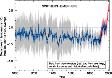
Figure 1: Multiproxy reconstruction of Northern Hemisphere surface temperature variations over the past millennium (blue), along with $40$-year average (black), a measure of the statistical uncertainty associated with the reconstruction (gray), and instrumental surface temperature (red), based on the work by Mann, Bradley and Hughes (1999). This figure has sometimes been referred to as the “hockey stick.” Source: IPCC (2001).

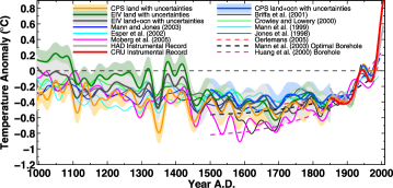
Figure 2: Various reconstructions of Northern Hemisphere temperatures over the last $1000$ years with $95$% confidence intervals. Source: Mann et al. (2008).

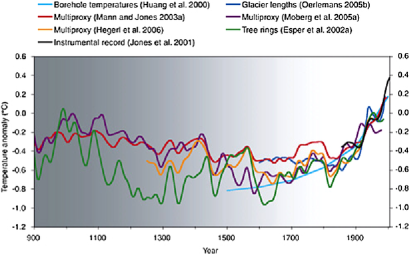
Figure 3: Smoothed reconstructions of large-scale (Northern Hemisphere mean or global mean) surface temperature variations from six different research teams are shown along with the instrumental record of global mean surface temperature. Each curve portrays a somewhat different history of temperature variations and is subject to a somewhat different set of uncertainties that generally increase going backward in time (as indicated by the gray shading). Source: NRC (2006).

It is not necessary to know very much about the underlying methods to see that graphs such as Figure 1 are problematic as descriptive devices. First, the superposition of the instrumental record (red) creates a strong but entirely misleading contrast. The blue historical reconstruction is necessarily smoother with less overall variation than the red instrumental record since the reconstruction is, in a broad sense, a weighted average of all global temperature histories conditional on the observed proxy record. Second, the blue curve closely matches the red curve during the period 1902 AD to 1980 AD because this period has served as the training data and therefore the blue curve is calibrated to the red during it (note also the red curve is plotted from 1902 AD to 1998 AD). This sets up the erroneous visual expectation that the reconstructions are more accurate than they really are. A careful viewer would know to temper such expectations by paying close attention to the reconstruction error bars given by the wide gray regions. However, even these are misleading because these are, in fact, pointwise confidence intervals and not confidence curves for the entire sample path of surface temperature. Furthermore, the gray regions themselves fail to account for model uncertainty.

2 Controversy

With so much at stake both financially and ecologically, it is not surprising that these analyses have provoked several controversies. While some have recently erupted in the popular press [Jolis (2009), Johnson (2009), Johnson and Naik (2009)], we root our discussion of these controversies and their history as they unfolded in the academic and scientific literature.

The first major controversy erupted when McIntyre and McKitrick (M&M) successfully replicated the Mann, Bradley and Hughes (1998) study [McIntyre and McKitrick (2003, 2005a, 2005b)]. M&M observed that the original Mann, Bradley and Hughes (1998) study (i) used only one principal component of the proxy record and (ii) calculated the principal components in a “skew”-centered fashion such that they were centered by the mean of the proxy data over the instrumental period (instead of the more standard technique of centering by the mean of the entire data record). Given that the proxy series is itself auto-correlated, this scaling has the effect of producing a first principal component which is hockey-stick shaped [McIntyre and McKitrick (2003)] and, thus, hockey-stick shaped temperature reconstructions. That is, the very method used in Mann, Bradley and Hughes (1998) guarantees the shape of Figure 1. M&M made a further contribution by applying the Mann, Bradley and Hughes (1998) reconstruction methodology to principal components computed in the standard fashion. The resulting reconstruction showed a rise in temperature in the medieval period, thus eliminating the hockey stick shape.

Mann and his colleagues vigorously responded to M&M to justify the hockey stick [Mann, Bradley and Hughes (2004)]. They argued that one should not limit oneself to a single principal component as in Mann, Bradley and Hughes (1998), but, rather, one should select the number of principal components retained through cross-validation on two blocks of heldout instrumental temperature records (i.e., the first 50 years of the instrumental period and the last 50 years). When this procedure is followed, four principal components are retained, and the hockey stick re-emerges even when the PCs are calculated in the standard fashion. Since the hockey stick is the shape selected by validation, climate scientists argue it is therefore the correct one.

The furor reached such a level that Congress took up the matter in 2006.

The Chairman of the Committee on Energy and Commerce and that of the Subcommittee on Oversight and Investigations formed an ad hoc committee of statisticians to review the findings of M&M. Their Congressional report [Wegman, Scott and Said (2006)] confirmed M&M’s finding regarding skew-centered principal components (this finding was yet again confirmed by the National Research Council [NRC (2006)]).

In his Congressional testimony [Wegman (2006)], committee chairman Edward Wegman excoriated Mann, Bradley and Hughes (2004) for use of additional principal components beyond the first after it was shown that their method led to spurious results:

In the MBH original, the hockey stick emerged in PC1 from the bristlecone/foxtail pines. If one centers the data properly the hockey stick does not emerge until PC4. Thus, a substantial change in strategy is required in the MBH reconstruction in order to achieve the hockey stick, a strategy which was specifically eschewed in MBH… a cardinal rule of statistical inference is that the method of analysis must be decided before looking at the data. The rules and strategy of analysis cannot be changed in order to obtain the desired result. Such a strategy carries no statistical integrity and cannot be used as a basis for drawing sound inferential conclusions.

Michael Mann, in his rebuttal testimony before Congress, admitted to having made some questionable choices in his early work. But, he strongly asserted that none of these earlier problems are still relevant because his original findings have been confirmed again and again in subsequent peer reviewed literature by large numbers of highly qualified climate scientists using vastly expanded data records [e.g., Mann and Rutherford (2002), Luterbacher et al. (2004), Mann et al. (2005, 2007, 2008), Rutherford et al. (2005), Wahl and Amman (2006), Wahl, Ritson and Amman (2006), Li, Nychka and Amman (2007)] even if criticisms do exist [e.g., von Storch et al. (2004)].

The degree of controversy associated with this endeavor can perhaps be better understood by recalling Wegman’s assertion that there are very few mainstream statisticians working on climate reconstructions [Wegman, Scott and Said (2006)]. This is particularly surprising not only because the task is highly statistical but also because it is extremely difficult. The data is spatially and temporally autocorrelated. It is massively incomplete. It is not easily or accurately modeled by simple autoregressive processes. The signal is very weak and the number of covariates greatly outnumbers the number of independent observations of instrumental temperature. Much of the analysis in this paper explores some of the difficulties associated with model selection and prediction in just such contexts. We are not interested at this stage in engaging the issues of data quality. To wit, henceforth and for the remainder of the paper, we work entirely with the data from Mann et al. (2008).

This is by far the most comprehensive publicly available database of temperatures and proxies collected to date. It contains 1209 climate proxies (with some going back as far as 8855 BC and some continuing up till 2003 AD). It also contains a database of eight global annual temperature aggregates dating 1850–2006 AD (expressed as deviations or “anomalies” from the 1961–1990 AD average). Finally, there is a database of 1732 local annual temperatures dating 1850–2006 AD (also expressed as anomalies from the 1961–1990 AD average). All three of these datasets have been substantially processed including smoothing and imputation of missing data [Mann et al. (2008)]. While these present interesting problems, they are not the focus of our inquiry. We assume that the data selection, collection, and processing performed by climate scientists meets the standards of their discipline. Without taking a position on these data quality issues, we thus take the dataset as given. We further make the assumptions of linearity and stationarity of the relationship between temperature and proxies, an assumption employed throughout the climate science literature [NRC (2006)] noting that “the stationarity of the relationship does not require stationarity of the series themselves” [NRC (2006)]. Even with these substantial assumptions, the paleoclimatological reconstructive endeavor is a very difficult one and we focus on the substantive modeling problems encountered in this setting.

Our paper structure and major results are as follows. We first discuss the strength of the proxy signal in this $p\gg n$ context (i.e., when the number of covariates or parameters, $p$, is much larger than the number of datapoints, $n$) by comparing the performance, in terms of holdout RMSE, of the proxies against several alternatives. Such an exercise is important because, when $p\gg n$, there is a sizeable risk of overfitting and in-sample performance is often a poor benchmark for out-of-sample performance. We will show that the proxy record easily does better at predicting out-of-sample global temperature than simple rapidly-mixing stationary processes generated independently of the true temperature record. On the other hand, the proxies do not fare so well when compared to predictions made by more complex processes also generated independently of any climate signal. That is, randomly generated sequences are as “predictive” of holdout temperatures as the proxies.

Next, we show that various models for predicting temperature can perform similarly in terms of cross-validated out-of-sample RMSE but have very different historical temperature backcasts. Some of these backcasts look like hockey sticks while others do not. Thus, cross-validation is inadequate on its own for model and backcast selection.

Finally, we construct and fit a full probability model for the relationship between the 1000-year-old proxy database and Northern Hemisphere average temperature, providing appropriate pathwise standard errors which account for parameter uncertainty. While our model offers support to the conclusion that the 1990s were the warmest decade of the last millennium, it does not predict temperature as well as expected even in-sample. The model does much worse on contiguous 30-year holdout blocks. Thus, we remark in conclusion that natural proxies are severely limited in their ability to predict average temperatures and temperature gradients.

All data and code used in this paper are provided in the supplementary materials [McShane and Wyner (2011)].

3 Model evaluation

3.1 Introduction

A critical difficulty for paleoclimatological reconstruction is that the temperature signal in the proxy record is surprisingly weak. That is, very few, if any, of the individual natural proxies, at least those that are uncontaminated by the documentary record, are able to explain an appreciable amount of the annual variation in the local instrumental temperature records. Nevertheless, the proxy record is quite large, creating an additional challenge: there are many more proxies than there are years in the instrumental temperature record. In this setting, it is easy for a model to overfit the comparatively short instrumental record and therefore model evaluation is especially important. Thus, the main goals of this section are twofold. First, we endeavor to judge regression-based methods for the specific task of predicting blocks of temperatures in the instrumental period. Second, we study specifically how the determination of statistical significance varies under different specifications of the null distribution.

Because the number of proxies is much greater than the number of years for which we have temperature data, it is unavoidable that some type of dimensionality reduction is necessary even if there is no principled way to achieve this. As mentioned above, early studies [Mann, Bradley and Hughes (1998, 1999)] used principal components analysis for this purpose. Alternatively, the number of proxies can be lowered through a threshold screening process [Mann et al. (2008)] whereby each proxy sequence is correlated with its closest local temperature series and only those proxies whose correlation exceeds a given threshold are retained for model building. This is a reasonable approach, but, for it to offer serious protection from overfitting the temperature sequence, it is necessary to detect “spurious correlations.”

Figure 4: Simulated sample correlation coefficient distribution of two independent random walks. One thousand independent pairs of random walks each of length $149$ were sampled to generate the above histogram.

The problem of spurious correlation arises when one takes the correlation of two series which are themselves highly autocorrelated and is well studied in the time series and econometrics literature [Yule (1926), Granger and Newbold (1974), Phillips (1986)]. When two independent time series are nonstationary (e.g., random walk), locally nonstationary (e.g., regime switching), or strongly autocorrelated, then the distribution of the empirical correlation coefficient is surprisingly variable and is frequently large in absolute value (see Figure 4). Furthermore, standard model statistics (e.g., t-statistics) are inaccurate and can only be corrected when the underlying stochastic processes are both known and modeled (and this can only be done for special cases).

Figure 5: CRU Northern Hemisphere annual mean land temperature, CRU Southern Hemisphere annual mean land temperature, and four local temperatures the grids of which contain (i) Spitsbergen island in the Svalbard archipelago in the Artic, (ii) the north portion of the Omsk oblast in southwestern Siberia, (iii) Attu Island, the westernmost island in the Aleutian islands arcipelago, and (iv) Baysuat in the Aktobe Province, Kazakhstan. The x-axis gives the year and the y-axis gives the temperature anomaly from 1961–1990 AD average in degrees Celsius.

As can be seen in Figures 5 and 6, both the instrumental temperature record as well as many of the proxy sequences are not appropriately modeled by low order stationary autoregressive processes. The dependence structure in the data is clearly complex and quite evident from the graphs. More quantitatively, we observe that the sample first-order autocorrelation of the CRU Northern Hemisphere annual mean land temperature series is nearly 0.6 (with significant partial autocorrelations out to lag four). Among the proxy sequences, a full one-third have empirical lag one autocorrelations of at least 0.5 (see Figure 7). Thus, standard correlation coefficient test statistics are not reliable measures of significance for screening proxies against local or global temperatures series. A final more subtle and salient concern is that, if the screening process involves the entire instrumental temperature record, it corrupts the model validation process: no subsequence of the temperature series can be truly considered out-of-sample.

To solve the problem of spurious correlation, climate scientists have used the technique of out-of-sample validation on a reserved holdout block of data. The performance of any given reconstruction can then be benchmarked and compared to the performance of various null models. This will be our approach as well. However, we extend their validation exercises by (i) expanding the class of null models and (ii) considering interpolated holdout blocks as well as extrapolated ones.

3.2 Preliminary evaluation

In this subsection, we discuss our validation scheme and compare the predictive performance of the proxies against two simple models which use only temperature itself for forecasting, the in-sample mean and ARMA models. We use as our response $y_{t}$ the CRU Northern Hemisphere annual mean land temperature. $X=\{x_{tj}\}$ is a centered and scaled matrix of 1138 of the 1209 proxies, excluding the 71 Lutannt series found in Luterbacher et al. (2004). We use the years 1850–1998 AD for these tests because very few proxies are available after 1998 AD.

Figure 6: Six proxy time series plotted during the instrumental period: speleothems in Scotland, monsoons in India, lake sediment in Ecuador; tree rings in Montana, dry/wet variation on the Yellow River, and lake sediments in Finland.

To assess the strength of the relationship between the natural proxies and temperature, we cross-validate the data. This is a standard approach, but our situation is atypical since the temperature sequence is highly autocorrelated. To mitigate this problem, we follow the approach of climate scientists in our initial approach and fit the instrumental temperature record using only proxy covariates. Nevertheless, the errors and the proxies are temporally correlated which implies that the usual method of selecting random holdout sets will not provide an effective evaluation of our model. Climate scientists have instead applied “block” validation, holding out two contiguous blocks of instrumental temperatures: a “front” block consisting of the first 50 years of the instrumental record and a “back” block consisting of the last 50 years.

Figure 7: Sample lag one autocorrelation coefficient for the 1209 proxies during the instrumental period.

On the one hand, this approach makes sense since our ultimate task is to extrapolate our data backward in time and only the first and last blocks can be used for this purpose specifically. On the other hand, limiting the validation exercise to these two blocks is problematic because both blocks have very dramatic and obvious features: the temperatures in the initial block are fairly constant and are the coldest in the instrumental record, whereas the temperatures in the final block are rapidly increasing and are the warmest in the instrumental record. Thus, validation conducted on these two blocks will prima facie favor procedures which project the local level and gradient of the temperature near the boundary of the in-sample period. However, while such procedures perform well on the front and back blocks, they are not as competitive on interior blocks. Furthermore, they cannot be used for plausible historical reconstructions! A final serious problem with validating on only the front and back blocks is that the extreme characteristics of these blocks are widely known; it can only be speculated as to what extent the collection, scaling, and processing of the proxy data as well as modeling choices have been affected by this knowledge.

Our approach is to consecutively select all possible contiguous blocks for holding out. For example, we take a given contiguous 30-year block from the 149-year instrumental temperature record (e.g., 1900–1929 AD) and hold it out. Using only the remaining 119 years (e.g, 1850–1899 AD and 1930–1998 AD), we tune and fit our model. Finally, we then use the fitted model to obtain predictions for each of the 30 years in the holdout block and then calculate the RMSE on this block.

We then repeat the procedure outlined in the previous paragraph over all 120 possible contiguous holdout blocks in order to approximate thedistribution of the holdout RMSE that is expected using this procedure. We note this test only gives a sense of the ability of the proxies to predict the instrumental temperature record and it says little about the ability of the proxies to predict temperature several hundred or thousand years back. Climate scientists have argued, however, that this long-term extrapolation is scientifically legitimate [Mann, Bradley and Hughes (1998), NRC (2006)].

Throughout this section, we assess the strength of the proxy signal by building models for temperature using the Lasso [Tibshirani (1996)]. The Lasso is a penalized least squares method which selects

$$\hat{\beta}^{\mathrm{Lasso}}=\operatorname{arg\min}\limits_{\beta}\Biggl{\{}\sum_{i=1}^{n}\Biggl{(}y_{i}-\beta_{0}-\sum_{j=1}^{p}x_{ij}\beta_{j}\Biggr{)}^{2}+\lambda\sum_{i=1}^{p}|\beta_{i}|\Biggr{\}}.$$

As can be seen, the intercept $\beta_{0}$ is not penalized. Typically (and in this paper), the matrix of predictors $X$ is centered and scaled, and $\lambda$ is chosen by cross-validation. Due to the $L_{1}$ penalty, the Lasso tends to choose sparse $\hat{\beta}^{\mathrm{Lasso}}$, thus serving as a variable selection methodology and alleviating the $p\gg n$ problem. Furthermore, since the Lasso tends to select only a few of a set of correlated predictors, it also helps reduce the problem of spatial correlation among the proxies.

We select the Lasso tuning parameter $\lambda$ by performing ten repetitions of five-fold cross-validation on the 119 in-sample years and choosing the value $\lambda=\hat{\lambda}$ which provides the best RMSE. We then fit the Lasso to the full 119-year in-sample dataset using $\lambda=\hat{\lambda}$ to obtain $\hat{\beta}^{\mathrm{Lasso}}$. Finally, we can use $\hat{\beta}^{\mathrm{Lasso}}$ to obtain predictions for each of the 30 years in the holdout block and then calculate the RMSE on this block.

We chose the Lasso because it is a reasonable procedure that has proven powerful, fast, and popular, and it performs comparably well in a $p\gg n$ context. Thus, we believe it should provide predictions which are as good or better than other methods that we have tried (evidence for this is presented in Figure 12). Furthermore, we are as much interested in how the proxies fare as predictors when varying the holdout block and null distribution (see Sections 3.3 and 3.4) as we are in performance. In fact, all analyses in this section have been repeated using modeling procedures other than the Lasso and qualitatively all results remain more or less the same.

As an initial test, we compare the holdout RMSE using the proxies to two simple models which only make use of temperature data, the in-sample mean and ARMA models. First, the proxy model and the in-sample mean seem to perform fairly similarly, with the proxy-based model beating the sample mean on only 57% of holdout blocks. A possible reason the sample mean performs comparably well is that the instrumental temperature record has a great deal of annual variation which is apparently uncaptured by the proxy record. In such settings, a biased low-variance predictor (such as the in-sample mean) can often have a lower out-of-sample RMSE than a less biased but more variable predictor. Finally, we observe that the performance on different validation blocks are not independent, an issue which we return to in Section 3.4.

We also compared the holdout RMSE of the proxies to another more sophisticated model which, like the in-sample mean, only makes use of temperature data and makes no reference to proxy data. For each holdout block, we fit various ARMA($p$, $q$) models; we let $p$ and $q$ range from zero to five and chose the values which give the best AIC. We then use this model to forecast the temperature on the holdout block. This model beats the proxy model 86% of the time.

Figure 8: CRU Northern Hemisphere annual mean land temperature is given by the thin black line and a smoothed version is given by the thick black line. The forecast produced by applying the Lasso to the proxies is given by the thin red line and a smoothed version is given by the thick red line. The in-sample mean is given by the horizontal blue line. The forecast produced by ARMA modeling is given by the thin green line and a smoothed version is given by the thick green line. The Lasso and ARMA models and the mean are fit on 1850–1968 AD and forecast on 1969–1998 AD.

In Figure 8, we focus on one particular holdout block, the last 30 years of the series. The in-sample mean and the ARMA model completely miss the rising trend of the last 30 years; in fact, both models are essentially useless for backcasting and forecasting since their long-term prediction is equal to the in-sample mean. On the other hand, the record of 1138 proxies does appear to capture the rising trend in temperatures (in the sequel, we will assess the statistical significance of this). Furthermore, the differences in temperature and the differences in the proxy forecast are significantly correlated ($p=0.021$), with the same sign in 21 out of the 29 years ($p=0.026$).

3.3 Validation against pseudo-proxies

Because both the in-sample mean and the ARMA model always forecast the mean in the long-term, they are not particularly useful models for the scientific endeavor of temperature reconstruction. Furthermore, the fact that the Lasso-selected linear combination of the proxies beats the in-sample mean on 57% of holdout blocks and the ARMA model on 14% of holdout blocks is difficult to interpret without solid benchmarks of performance.

One way to provide benchmarks is to repeat the Lasso procedure outlined above using 1138 “pseudo-proxies” in lieu of the 1138 real proxies. That is, replace the natural proxies of temperature by an alternate set of time series. Any function of the proxies, with their resultant temperature reconstruction, can be validated by comparing the ability of the proxies to predict out-of-sample instrumental temperatures to the ability of the pseudo-proxies.

The use of pseudo-proxies is quite common in the climate science literature where pseudo-proxies are often built by adding an AR1 time series (“red noise”) to natural proxies, local temperatures, or simulated temperatures generated from General Circulation Models [Mann and Rutherford (2002), Wahl and Amman (2006)]. These pseudo-proxies determine whether a given reconstruction is “skillful” (i.e., statistically significant). Skill is demonstrated with respect to a class of pseudo-proxies when the true proxies outperform the pseudo-proxies with high probability (probabilities are approximated by simulation). In our study, we use an even weaker benchmark than those in the climate science literature: our pseudo-proxies are random numbers generated completely independently of the temperature series.

The simplest class of pseudo-proxies we consider are Gaussian White Noise. That is, we apply the Lasso procedure outlined above to a $149\times 1138$ matrix of standard normal random variables. Formally, let $\varepsilon_{t}\stackrel{{\scriptstyle\mathrm{i.i.d.}}}{{\sim}}N(0,1),t=1,2,\ldots.$ Then, our White Noise pseudo-proxies are defined as $X_{t}\equiv\varepsilon_{t}$ and we generate 1138 such series, each of length 149.

We also consider three classes of AR1 or “red noise” pseudo-proxies since they are common in the climate literature [Mann, Bradley and Hughes (1998), von Storch et al. (2004), Mann et al. (2008)]. Again, if $\varepsilon_{t}\stackrel{{\scriptstyle\mathrm{i.i.d.}}}{{\sim}}N(0,1)$, then an AR1 pseudo-proxy is defined as $X_{t}\equiv\phi X_{t-1}+\varepsilon_{t}$. Two of the classes are AR1 with the $\phi$ coefficient set in turn to 0.25 and 0.4 [these are the average sample proxy autocorrelations reported in Mann, Bradley and Hughes (1998) and Mann et al. (2008), resp.]. The third class is more complicated. First, we fit an AR1 model to each of the 1138 proxies and calculate the sample AR1 coefficients $\hat{\phi}_{1},\ldots,\hat{\phi}_{1138}$. Then, we generate an AR1 series setting $\phi=\hat{\phi}_{i}$ for each of these 1138 estimated coefficients. We term this the empirical AR1 process. This approach is similar to that of McIntyre and McKitrick (2005a, 2005c) who use the full empirical autocorrelation function to generate trend-less pseudo-proxies.

We also consider Brownian motion pseudo-proxies formed by taking the cumulative sums of $N(0,1)$ random variables. That is, if $\varepsilon_{t}\stackrel{{\scriptstyle\mathrm{i.i.d.}}}{{\sim}}N(0,1)$, then a Brownian motion pseudo-proxy is defined as $X_{t}\equiv\sum_{j=1}^{t}\varepsilon_{j}=X_{t-1}+\varepsilon_{t}$.

White Noise and Brownian motion can be thought of as special cases of AR1 pseudo-proxies. In fact, they are the extrema of AR1 processes: White Noise is AR1 with the $\phi$ coefficient set to zero and Brownian motion is AR1 with the $\phi$ coefficient set to one.

Before discussing the results of these simulations, it is worth emphasizing why this exercise is necessary. That is, why can’t one evaluate the model using standard regression diagnostics (e.g., F-statistics, t-statistics, etc.)? One cannot because of two problems mentioned above: (i) the $p\gg n$ problem and (ii) the fact that proxy and temperature autocorrelation causes spurious correlation and therefore invalid model statistics (e.g., t-statistics). The first problem has to be dealt with via dimensionality reduction; the second can only be solved when the underlying processes are known (and then only in special cases).

Given that we do not know the true underlying dynamics, the nonparametric, prediction-based approach used here is valuable. We provide a variety of benchmark pseudo-proxy series and obtain holdout RMSE distributions. Since these pseudo-proxies are generated independently of the temperature series, we know they cannot be truly predictive of it. Hence, the real proxies—if they contain linear signal on temperatures—should outperform our pseudo-proxies, at least with high probability.

For any given class of pseudo-proxy, we can estimate the probability that a randomly generated pseudo-proxy sequence outperforms the true proxy record for predicting temperatures in a given holdout block. A major focus of our investigation is the sensitivity of this outperformance “p-value” to various factors. We proceed in two directions. We first consider the level and variability in holdout RMSE for our various classes of pseudo-proxies marginally over all 120 holdout blocks. Second, since these 120 holdout blocks are highly correlated with one another, we study how the holdout RMSE varies from block to block in Section 3.4.

Figure 9: Cross-validated RMSE on $30$-year holdout blocks for various models fit to proxies and pseudo-proxies. The procedures used to generate the Proxy, Intercept, and ARMA boxplots are discussed in Section 3.2. The procedures used to generate the White Noise, AR1, and Brownian motion boxplots are discussed in Section 3.3. The procedure used to generate the Grid Proxy boxplot is discussed in Section 3.6.

We present our results in Figure 9, with the RMSE boxplot for the proxies given first. As can be seen, the proxies have a slightly worse median RMSE than the intercept-only model (i.e., the in-sample mean) but the distribution is narrower. On the other hand, the ARMA model is superior to both. When the Lasso is used on White Noise pseudo-proxies, the performance is similar to the intercept-only model because the Lasso is choosing a very parsimonious model.

The proxies seem to outperform the AR1(0.25) and AR1(0.4) models, with both a better median and a lower variance. While this is encouraging, it is also raises a concern: AR1(0.25) and AR1(0.4) are the models frequently used as “null benchmarks” in the climate science literature and they seem to perform worse than both the intercept-only and White Noise benchmarks. This suggests that climate scientists are using a particularly weak null benchmark to test their models. That the null models may be too weak and the associated standard errors in papers such as Mann, Bradley and Hughes (1998) are not wide enough has already been pointed out in the climate literature [von Storch et al. (2004)]. While there was some controversy surrounding the result of this paper [Wahl, Ritson and Amman (2006)], its conclusions have been corroborated [von Storch and Zorita (2005), von Storch et al. (2006), Lee, Zwiers and Tsao (2008), Christiansen, Schmith and Thejll (2009)].

Finally, the empirical AR1 process and Brownian motion both substantially outperform the proxies. They each have a lower average holdout RMSE and lower variability than that achieved by the proxies. This is extremely important since these two classes of time series are generated completely independently of the temperature data. They have no long term predictive ability, and they cannot be used to reconstruct historical temperatures. Yet, they significantly outperform the proxies at 30-year holdout prediction!

In other words, our model performs better when using highly autocorrelated noise rather than proxies to “predict” temperature. The real proxies are less predictive than our “fake” data. While the Lasso-generated reconstructions using the proxies are highly statistically significant compared to simple null models, they do not achieve statistical significance against sophisticated null models.

We are not the first to observe this effect. It was shown, in McIntyre and McKitrick (2005a, 2005c), that random sequences with complex local dependence structures can predict temperatures. Their approach has been roundly dismissed in the climate science literature:

To generate “random” noise series, MM05c apply the full autoregressive structure of the real world proxy series. In this way, they in fact train their stochastic engine with significant (if not dominant) low frequency climate signal rather than purely nonclimatic noise and its persistence. [Emphasis in original]

Ammann and Wahl (2007)

Broadly, there are two components to any climate signal. The first component is the local time dependence made manifest by the strong autocorrelation structure observed in the temperature series itself. It is easily observed that short term future temperatures can be predicted by estimates of the local mean and its first derivatives [Green, Armstrong and Soon (2009)]. Hence, a procedure that fits sequences with complex local dependencies to the instrumental temperature record will recover the ability of the temperature record to self-predict in the short run.

The second component—long-term changes in the temperature series—can, on the other hand, only be predicted by meaningful covariates. The autocorrelation structure of the temperature series does not allow for self-prediction in the long run. Thus, pseudo-proxies like ours, which inherit their ability at short-term prediction by borrowing the dependence structure of the instrumental temperature series, have no more power to reconstruct temperature than the instrumental record itself (which is entirely sensible since these pseudo-proxies are generated independently of the temperature series).

Ammann and Wahl (2007) claim that significance thresholds set by Monte Carlo simulations that use pseudo-proxies containing “short term climate signal” (i.e., complex time dependence structures) are invalid:

Such thresholds thus enhance the danger of committing Type II errors (inappropriate failure to reject a null hypothesis of no climatic information for a reconstruction).

We agree that these thresholds decrease power. Still, these thresholds are the correct way to preserve the significance level. The proxy record has to be evaluated in terms of its innate ability to reconstruct historical temperatures (i.e., as opposed to its ability to “mimic” the local time dependence structure of the temperature series). Ammann and Wahl (2007) wrongly attribute reconstructive skill to the proxy record which is in fact attributable to the temperature record itself. Thus, climate scientists are overoptimistic: the 149-year instrumental record has significant local time dependence and therefore far fewer independent degrees of freedom.

3.4 Interpolation versus extrapolation

In our analysis, we expanded our set of holdout blocks to include all contiguous 30-year blocks. The benefits of this are twofold. First, this expansion increases our sample size from two (the front and back blocks) to 120 (because there are 118 possible interior blocks). Second, by expanding the set of holdout blocks, we mitigate the potential effects of data snooping since salient characteristics of the first and last blocks are widely known. On the other hand, this expansion imposes difficulties. The RMSEs of overlapping blocks are highly dependent. Furthermore, since temperatures are autocorrelated, the RMSEs of neighboring nonoverlapping blocks are also dependent. Thus, there is little new information in each block. We explore this graphically by plotting the RMSE of each holdout block against the first year of the block in Figure 10.

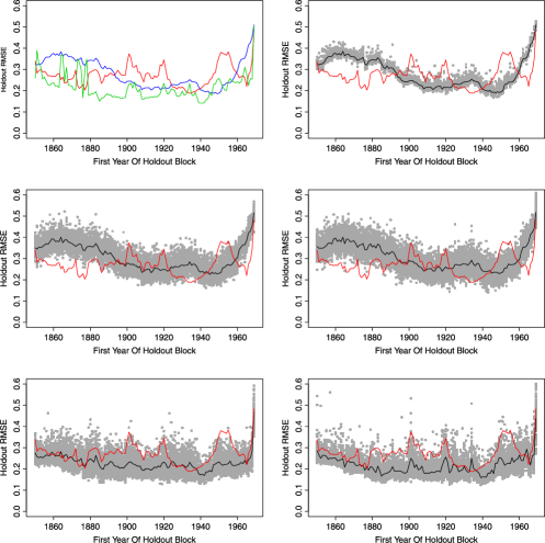
Figure 10: Holdout RMSE by first year of holdout block. In all panels, the Lasso-selected linear combination of the proxies is given in red. In the upper-left panel, the in-sample mean is given in blue and the ARMA model in green. In the upper-right panel, the average for the White Noise pseudo-proxy is given in black. In the middle-left panel, the average for the $\operatorname{AR1}(0.25)$ pseudo-proxy is given in black. In the middle-right panel, the average for the $\operatorname{AR1}(0.4)$ pseudo-proxy is given in black. In the lower-left panel, the average for the Empirical $AR1$ pseudo-proxy is given in black. In the lower-right panel, the average for the Brownian motion pseudo-proxy is given in black. Confidence intervals for the pseudo-proxies are given in gray and are formed by taking $100$ samples of the pseudo-proxy matrix for each holdout block.

We begin our discussion by comparing RMSE of the Lasso model fitted to the proxies to RMSE of the in-sample mean and the RMSE of the ARMA model in upper left panel of Figure 10. As can be seen, the ARMA model either dominates or is competitive on every holdout block. The proxies, on the other hand, can match the performance of the ARMA model only on the first 20 or so holdout blocks, but on other blocks, they perform quite a bit worse.

More interesting is the examination of the performance of the pseudo-proxies, as shown in the remaining five panels of Figure 10. In these graphs, we compare the RMSE of the proxies on each holdout block to the RMSE of the pseudo-proxies. We also provide confidence intervals for the pseudo-proxies at each block by simulating 100 draws of the pseudo-proxy matrix and repeating our fitting procedure to each draw. As can be seen in the upper-right panel, the proxies show statistically significant improvement over White Noise for many of the early holdout blocks as well as many of the later ones. However, there are blocks, particularly in the middle, where they perform significantly worse.

When the AR1(0.25) and AR1(0.4) pseudo-proxies preferred by climate scientists are used, the average RMSE on each is comparable to that given by White Noise but the variation is considerably higher as shown by the middle two panels of Figure 10. Hence, the proxies perform statistically significantly better on very few holdout blocks, particularly those near the beginning of the series and those near the end. This is a curious fact because the “front” holdout block and the “back” holdout block are the only two which climate scientists use to validate their models. Insofar as this front and back performance is anomalous, they may be overconfident in their results.

Finally, we consider the AR1 Empirical and Brownian motion pseudo-proxies in the lower two panels of Figure 10. For almost all holdout blocks, these pseudo-proxies have an average RMSE that is as low or lower than that of the proxies. Further, for no block is the performance of true proxies statistically significantly better than that of either of these pseudo-proxies. Hence, we cannot reject the null hypothesis that the true proxies “predict” equivalently to highly correlated and/or nonstationary sequences of random noise that are independent of temperature.

A little reflection is in order. By cross-validating on interior blocks, we are able to greatly expand the validation test set. However, reconstructing interior blocks is an interpolation of the training sequence and paleoclimatological reconstruction requires extrapolation as opposed to interpolation. Pseudo-proxy reconstructions can only extrapolate a climate trend accurately for a very short period and then only insofar as the local dependence structure in the pseudo-proxies matches the local dependence structure in the temperature series. That is, forecasts from randomly generated series can extrapolate successfully only by chance and for very short periods.

On the other hand, Brownian motions and other pseudo-proxies with strong local dependencies are quite suited to interpolation since their in-sample forecasts are fitted to approximately match the the training sequence datapoints that are adjacent to the initial and final points of a test block. Nevertheless, true proxies also have strong local dependence structure since they are temperature surrogates and therefore should similarly match these datapoints of the training sequence. Furthermore, unlike pseudo-proxies, true proxies are not independent of temperature (in fact, the scientific presumption is that they are predictive of it). Therefore, proxy interpolations on interior holdout blocks should be expected to outperform pseudo-proxy forecasts notwithstanding the above.

3.5 Variable selection: True proxies versus pseudo-proxies

While the use of noise variables such as the pseudo-proxies is not unknown in statistics, such variables have typically been used to augment a matrix of covariates rather than to replace it. For example, Wu, Boos and Stefanski (2007) augment a matrix of covariates with noise variables in order to tune variable selection methodologies. Though that is not our focus, we make use of a similar approach in order to assess the the degree of signal in the proxies.

We first augment the in-sample matrix of proxies with a matrix of pseudo-proxies of the same size (i.e., replacing the $119\times 1138$ proxy matrix with a matrix of size $119\times 2276$ which consists of the original proxies plus pseudo-proxies). Then, we repeat the Lasso cross-validation described in Section 3.2, calculate the percent of variables selected by the Lasso which are pseudo-proxies, and average over all 120 possible blocks. If the signal in the proxies dominates that in the pseudo-proxies, then this percent should be relatively close to zero.

=174pt Pseudo-proxy Percent selected White Noise 37.8% AR1(0.25) 43.5% AR1(0.4) 47.9% Empirical AR1 53.0% Brownian Motion 27.9%

Table 1: Percent of pseudo-proxies selected by the Lasso

Table 1 shows this is far from the case. In general, the pseudo-proxies are selected about as often as the true proxies. That is, the Lasso does not find that the true proxies have substantially more signal than the pseudo-proxies.

3.6 Proxies and local temperatures

We performed an additional test which accounts for the fact that proxies are local in nature (e.g., tree rings in Montana) and therefore might be better predictors of local temperatures than global temperatures. Climate scientists generally accept the notion of “teleconnection” (i.e., that proxies local to one place can be predictive of climate in another possibly distant place). Hence, we do not use a distance restriction in this test. Rather, we perform the following procedure.

Again, let $y_{t}$ be the CRU Northern Hemisphere annual mean land temperature where $t$ indexes each year from 1850–1998 AD, and let $X=\{x_{tj}\}$ be the centered and scaled matrix of 1138 proxies from 1850–1998 AD where $t$ indexes the year and $j$ indexes each proxy. Further, let $Z=\{z_{tj}\}$ to be the matrix of the 1732 centered and scaled local annual temperatures from 1850–1998 AD where again $t$ indexes the year and $j$ indexes each local temperature.

As before, we take a 30-year contiguous block and reserve it as a holdout sample. Our procedure has two steps:

1. Using the 119 in-sample years, we perform ten repetitions of five-fold cross-validation as described in Section 3.2. In this case, however, instead of using the proxies $X$ to predict $y$, we use the local temperatures $Z$. As before, this procedure gives us an optimal value for the tuning parameter $\hat{\lambda}$ which we can use on all 119 observations of $y$ and $Z$ to obtain $\hat{\beta}^{\mathrm{Lasso}}$.

2. Now, for each $j$ such that $\hat{\beta}^{\mathrm{Lasso}}_{j}\neq 0$, we create a Lasso model for $z_{\cdot j}$. That is, we perform ten repetitions of five-fold cross-validation as in Section 3.2 but using $X$ to predict $z_{\cdot j}$. Again, this procedure gives us an optimal value for the tuning parameter $\hat{\lambda}_{j}$ which we can use on all 119 observations of $z_{\cdot j}$ and $X$ to obtain $\hat{\beta}^{\mathrm{Lasso},(j)}$.

Similarly, we can predict on the holdout block using a two-stage procedure. For each $j$ such that $\hat{\beta}^{\mathrm{Lasso}}_{j}\neq 0$, we apply $\hat{\beta}^{\mathrm{Lasso},(j)}$ to $X$ to obtain $\hat{z}_{\cdot j}$ in the 30 holdout years. Then, we apply $\hat{\beta}^{\mathrm{Lasso}}$ to the collection of $\hat{z}_{\cdot j}$ in order to obtain $\hat{y}_{t}$ in the 30 holdout years. Finally, we calculate the RMSE on the holdout block and repeat this procedure over all 120 possible holdout blocks.

As in Section 3.2, this procedure uses the Lasso to mitigate the $p\gg n$ problem. Furthermore, since the Lasso is unlikely to select correlated predictors, it also attenuates the problem of spatial correlation among the local temperatures and proxies. But, this procedure has the advantage of relating proxies to local temperatures, a feature which could be advantageous if these relationships are more conspicuous and enduring than those between proxies and the CRU global average temperature. The same is also potentially true mutatis mutandis of the relationship between the local temperatures and CRU.

The results of this test are given by the second boxplot in Figure 9. As can be seen, this method seems to perform somewhat better than the pure global method. However, it does not beat the empirical AR1 process or Brownian motion. That is, random series that are independent of global temperature are as effective or more effective than the proxies at predicting global annual temperatures in the instrumental period. Again, the proxies are not statistically significant when compared to sophisticated null models.

3.7 Discussion of model evaluation

We can think of four possible explanatory factors for what we have observed. First, it is possible that the proxies are in fact too weakly connected to global annual temperature to offer a substantially predictive (as well as reconstructive) model over the majority of the instrumental period. This is not to suggest that proxies are unable to detect large variations in global temperature (such as those that distinguish our current climate from an ice age). Rather, we suggest it is possible that natural proxies cannot reliably detect the small and largely unpredictable changes in annual temperature that have been observed over the majority of the instrumental period. In contrast, we have previously shown that the proxy record has some ability to predict the final 30-year block, where temperatures have increased most significantly, better than chance would suggest.

A second explanation is that the Lasso might be a poor procedure to apply to these data. This seems implausible both because the Lasso has been used successfully in a variety of $p\gg n$ contexts and because we repeated the analyses in this section using modeling strategies other than the Lasso and obtained the same general results. On the other hand, climate scientists have basically used three different statistical approaches: (i) scaling and averaging (so-called “Composite Plus Scale” or CPS) [NRC (2006)], (ii) principal component regression [NRC (2006)], and (iii) “Errors in Variables” (EIV) regression [Schneider (2001), Mann et al. (2007)]. The EIV approach is considered the most reliable and powerful. The approach treats forecasting (or reconstruction) from a missing data perspective using the Expectation–Maximization algorithm to “fill-in” blocks of missing values. The EM core utilizes an EIV generalized linear regression which addresses the $p\gg n$ problem using regularization in the form of a ridge regression-like total sum of squares constraint (this is called “RegEM” in the climate literature [Mann et al. (2007)]). All of these approaches are intrinsically linear, like Lasso regression, although the iterative RegEM can produce nonlinear functions of the covariates. Fundamentally, there are only theoretical performance guarantees for i.i.d. observations, while our data is clearly correlated across time. The EM algorithm in particular lacks a substantive literature on accuracy and performance without specific assumptions on the nature of missing data. Thus, it not obvious why the Lasso regression should be substantively worse than these methods. Nevertheless, in subsequent sections we will study a variety of different and improved model variations to confirm this.

A third explanation is that our class of competitive predictors (i.e., the pseudo-proxies) may very well provide unjustifiably difficult benchmarks as claimed by Ammann and Wahl (2007) and discussed in Section 3.3. Climate scientists have calibrated their performance using either (i) weak AR1 processes of the kind demonstrated above as pseudo-proxies or (ii) by adding weak AR1 processes to local temperatures, other proxies, or the output from global climate simulation models. In fact, we have shown that the the proxy record outperforms the former. On the other hand, weak AR1 processes underperform even white noise! Furthermore, it is hard to argue that a procedure is truly skillful if it cannot consistently outperform noise, no matter how artfully structured. In fact, Figure 6 reveals that the proxy series contain very complicated and highly autocorrelated time series structures which indicates that our complex pseudo-proxy competitors are not entirely unreasonable.

Finally, perhaps the proxy signal can be enhanced by smoothing various time series before modeling. Smoothing seems to be a standard approach for the analysis of climate series and is accompanied by a large body of literature [Mann (2004, 2008)]. Still, from a statistical perspective, smoothing time series raises additional questions and problems. At the most basic level, one has to figure out which series should be smoothed: temperatures, proxies, or both. Or, perhaps, only the forecasts should be smoothed in order to reduce the forecast variance. A further problem with smoothing procedures is that there are many methods and associated tuning parameters and there are no clear data-independent and hypothesis-independent methods of selecting among the various options. The instrumental temperature record is also very well known so there is no way to do this in a “blind” fashion. Furthermore, smoothing data exacerbates all of the statistical significance issues already present due to autocorrelation: two smoothed series will exhibit artificially high correlations and both standard errors and p-values require corrections (which are again only known under certain restrictive conditions).

4 Testing other predictive methods

4.1 Cross-validated RMSE

In this section, we pursue alternative procedures, including regression approaches more directly similar to techniques used by climate scientists. We shall see, working with a similar dataset, that various fitting methods can have both (i) very similar contiguous 30-year cross-validated instrumental period RMSE distributions and (ii) very different historical backcasts.

Again, we use as our response the CRU Northern Hemisphere annual mean land temperature from 1850–1998 AD and augment it with the 1732 local temperature series when required. However, since we are ultimately interested in large-scale reconstructions, we limit ourselves in this section to only those 93 proxies for which we have data going back over 1000 years. Hence, our in-sample dataset consists of the CRU global aggregate, the 1732 local temperatures, and the 93 proxies from 1850–1998 AD and we apply the cross-validation procedure discussed in Section 3.2 to it. We can then examine backcasts on the 998–1849 AD period for which only the proxies are available. We expect that our prediction accuracy during the instrumental period will decay somewhat since our set of proxies is so much smaller. However, the problem of millennial reconstructions is much more interesting both statistically and scientifically. It is well known and generally agreed that the several hundred years before the industrial revolution were a comparatively cool “Little Ice Age” [Matthes (1939), Lamb (1990)]. What happened in the early Medieval period is much more controversial and uncertain [Ladurie (1971), IPCC (2001)].

Figure 11: Cross-validated RMSE on $30$-year holdout blocks for various model specifications: intercept only and regression on the first one, five, ten, and $20$ principal components of the proxies.

We now examine how well the proxies predict under alternative model specifications. In the first set of studies, we examine RMSE distributions using an intercept-only model and ordinary least squares regression on the first one, five, ten, and 20 principal components calculated from the full $1001\times 93$ proxy matrix. Our results are shown in Figure 11. As can be seen, all of these methods perform comparably, with five and ten principal component models perhaps performing slightly better than the others.

Figure 12: Cross-validated RMSE on $30$-year holdout blocks for various model specifications: regression on the first ten principal components of the proxies, the Lasso applied to the proxies and the principal components of the proxies, stepwise regression to maximize AIC applied to the proxies and the principal components of the proxies, and stepwise regression to maximize BIC applied to the proxies and the principal components of the proxies.

In a second set of validations, we consider various variable selection methodologies and apply them to both the raw proxies and the principal components of the proxies. The methods considered are the Lasso and stepwise regression designed to optimize AIC and BIC, respectively. We plot our results in Figure 12 and include the boxplot of the ten principal component model from Figure 11 for easy reference. As can be seen, the stepwise models perform fairly similarly with one another. The Lasso performs slightly better and predicts about as well as the ten principal component model.

Figure 13: Cross-validated RMSE on $30$-year holdout blocks for various model specifications: regression on the first ten principal components of the proxies and various two-stage models where global temperature is regressed on principal components of local temperatures which are then regressed on principal components of proxies.

As a final consideration, we employ a method similar to that used in the original Mann, Bradley and Hughes (1998) paper. This method takes account of the fact that local proxies might be better predictors of local temperatures than they are of global aggregate temperatures. For this method, we again use the first $p$ principal components of the proxy matrix but we also use the first $g$ principal components of the $149\times 1732$ local temperature matrix. We regress the CRU global aggregate on the $g$ principal components of local temperature matrix, and then we regress each of the $g$ local temperature principal components on the $p$ proxy principal components. We can then use the historical proxy principal components to backcast the local temperature principal components thereby enabling us to backcast the global average temperature.

We plot our results in Figure 13 and again include the boxplot of ten principal components from Figure 11 for easy reference. As before, there is simply not that much variation in holdout RMSE across the various model specifications. No method is a clear winner.

4.2 Temperature reconstructions

Each model discussed in Section 4.1 can form a historical backcast. This backcast is simply the model’s estimate $\hat{y}_{k}(\mathbf{x}_{t})$ of the Northern Hemisphere average temperature in a year $t$ calculated by inputing the proxy covariates $\mathbf{x}_{t}$ in the same year. The model index is $k$ which varies over all 27 models from Section 4.1 (i.e., those featured in Figures 11–13). We plot these backcasts in Figure 14 in gray and show the CRU average in black. As can be seen, while these models all perform similarly in terms of cross-validated RMSE, they have wildly different implications about climate history.

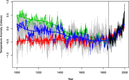
Figure 14: Backcasts to $1000$ AD from the various models considered in this section are plotted in gray. CRU Northern Hemisphere annual mean land temperature is given by the thin black line with a smoothed version given by the thick black line. Three forecasts are featured: regression on one proxy principal component (red), regression on ten proxy principal components (green), and the two-stage model featuring five local temperature principal components and five proxy principal components (blue).

According to some of them (e.g., the ten proxy principal component model given in green or the two-stage model featuring five local temperature principal components and five proxy principal components given in blue), the recent run-up in temperatures is not that abnormal, and similarly high temperatures would have been seen over the last millennium. Interestingly, the blue backcast seems to feature both a Medieval Warm Period and a Little Ice Age whereas the green one shows only increasing temperatures going back in time.

However, other backcasts (e.g., the single proxy principal component regression featured in red) are in fact hockey sticks which correspond quite well to backcasts such as those in Mann, Bradley and Hughes (1999). If they are correct, modern temperatures are indeed comparatively quite alarming since such temperatures are much warmer than what the backcasts indicate was observed over the past millennium.

Figure 14 reveals an important concern: models that perform similarly at predicting the instrumental temperature series (as revealed by Figures 11–13) tell very different stories about the past. Thus, insofar as one judges models by cross-validated predictive ability, one seems to have no reason to prefer the red backcast in Figure 14 to the green even though the former suggests that recent temperatures are much warmer than those observed over the past 1000 years while the latter suggests they are not.

A final point to note is that the backcasts plotted in Figure 14 are the raw backcasts themselves with no accounting for backcast standard errors. In the next section, we take on the problem of specifying a full probability model which will allow us to provide accurate, pathwise standard errors.

5 Bayesian reconstruction and validation

5.1 Model specification

In the previous section, we showed that a variety of different models perform fairly similarly in terms of cross-validated RMSE while producing very different temperature reconstructions. In this section, we focus and expand on the model which uses the first ten principal components of the proxy record to predict Northern Hemisphere CRU. We chose this forecast for several reasons. First, it performed relatively well compared to all of the others (see Figures 11–13). Second, PC regression has a relatively long history in the science of paleoclimatological reconstructions [Mann, Bradley and Hughes (1998, 1999), NRC (2006)]. Finally, when using OLS regression, principal components up to and including the tenth were statistically significant. While the t-statistics and their associated p-values themselves are uninterpretable due to the complex time series and error structures, these traditional benchmarks can serve as guideposts.

However, there is at least one serious problem with this model as it stands: the residuals demonstrate significant autocorrelation not captured by the autocorrelation in the proxies. Accordingly, we fit a variety of autoregressive models to CRU time series. With an AR2 model, the residuals showed very little autocorrelation.

So that we account for both parameter uncertainty as well as residual uncertainty, we estimate our model using Bayesian procedures. Our likelihood is given by

$$y_{t} = \beta_{0}+\sum_{i=1}^{10}\beta_{i}x_{t,i}+\beta_{11}y_{t+1}+\beta_{12}y_{t+2}+\varepsilon_{t},$$

$$\varepsilon_{t} \sim N(0,\sigma^{2}).$$

In our equation, $y_{t}$ represents the CRU Northern Hemisphere annual land temperature in year $t$ and $x_{t,i}$ is the value of principal component $i$ in year $t$. We note that the subscripts on the right-hand side of the regression equation employ pluses rather than the usual minuses because we are interested in backcasts rather than forecasts. In addition to this, we use the very weakly informative priors

$$\vec{\beta} \sim N(\vec{0},1000\cdot I),$$

$$\sigma \sim \operatorname{Unif}(0,100),$$

where $\vec{\beta}$ is the 13 dimensional vector $(\beta_{0},\beta_{1},\ldots,\beta_{12})^{T}$, $\vec{0}$ is a vector of 13 zeros, and $I$ is the 13 dimensional identity matrix. This prior is sufficiently noninformative that the posterior mean of $\vec{\beta}$ is, within rounding error, equal to the maximum likelihood estimate. Furthermore, the prior on $\sigma$ is effectively noninformative as $y_{t}$ is always between $\pm 1$ and therefore no posterior draw comes anywhere near the boundary of $100$.

It is important to consider how our model accounts for the perils of temperature reconstruction discussed above. First and foremost, we deal with the problem of weak signal by building a simple model ($\operatorname{AR}2+\mathrm{PC}10$) in order to avoid overfitting. Our fully Bayesian model, which accounts for parameter uncertainty, also helps attenuate some of the problems caused by weak signal. Dimensionality reduction is dealt with via principal components. PCs have two additional benefits. First, they are well-studied in the climate science literature and are used in climate scientists’ reconstructions. Second, the orthogonality of principal components will diminish the pernicious effects of spatial correlation among the proxies. Finally, we address the temporal correlation of the temperature series with the AR2 component of our model.

5.2 Comparison to other models

An approach that is broadly similar to the above has recently appeared in the climate literature [Li, Nychka and Amman (2007)] for purposes similar to ours, namely, quantifying the uncertainty of a reconstruction. In fact, Li, Nychka and Amman (2007) is highly unusual in the climate literature in that its authors are primarily statisticians. Using a dataset of 14 proxies from Mann, Bradley and Hughes (1999), Li, Nychka and Amman (2007) confirms the findings of Mann, Bradley and Hughes (1998, 1999) but attempts to take forecast error, parameter uncertainty, and temporal correlation into account. They provide toy data and code for their model here: http://www.image.ucar.edu/~boli/research.html

Nevertheless, several important distinctions between their model and ours exist. First, Li, Nychka and Amman (2007) make use of a dataset over ten years old [Mann, Bradley and Hughes (1999)] which contains only 14 proxies dating back to 1000 AD and has instrumental records dating 1850–1980 AD. On the other hand, we make use of the latest multi-proxy database [Mann et al. (2008)] which contains 93 proxies dating back to 1000 AD and has instrumental records dating 1850–1998 AD. Furthermore, Li, Nychka and Amman (2007) assume an AR2 structure on the errors from the model where we assume the model is AR2 with covariates. Finally, and perhaps most importantly, Li, Nychka and Amman (2007) estimate their model via generalized least squares and therefore use (i) the parametric bootstrap in order to account for parameter estimation uncertainty and (ii) cross-validation to account overfitting the in-sample period (i.e., to inflate their estimate of the error variance $\sigma$). On the other hand, by estimating our model in a fully Bayesian fashion, we can account for these within our probability model. Thus, our procedure can be thought of as formalizing the approach of Li, Nychka and Amman (2007) and it provides practically similar results when applied to the same set of covariates (generalized least squares also produced practically indistinguishable forecasts and backcasts though obviously narrower standard errors).

At the time of this manuscript’s submission, the same authors were working on a fully Bayesian model which deserves mention [subsequently published as Li, Nychka and Amman (2010)]. In this paper, they integrate data from three types of proxies measured at different timescales (tree rings, boreholes, and pollen) as well as data from climate forcings (solar irradiance, volcanism, and greenhouse gases) which are considered to be external drivers of climate. Furthermore, they account for autocorrelated error in both the proxies and forcings as well as autocorrelation in the deviations of temperature from the model. While the methodology and use of forcing data are certainly innovative, the focus of Li, Nychka and Amman (2010) is not on reconstruction per se; rather, they are interested in validating their modeling approach taking as “truth” the output of a high-resolution state-of-the-art climate simulation [Amman et al. (2007)]. Consequently, all data used in the paper is synthetic and they concentrate on methodological issues, “defer[ring] any reconstructions based on actual observations and their geophysical interpretation to a subsequent paper” [Li, Nychka and Amman (2010)].

Finally, Tingley and Huybers (2010a, 2010b) have developed a hierarchical Bayesian model to reconstruct the full temperature field. They fit the model to experimental datasets formed by “corrupting a number of the [temperature] time series to mimic proxy observations” [Tingley and Huybers (2010a)]. Using these datasets, they conduct what is in essence a frequentist evaluation of their Bayesian model [Tingley and Huybers (2010a)] and then compare its performance to that of the well-known RegEM algorithm [Tingley and Huybers (2010b)]. Like Li, Nychka and Amman (2010), however, they do not use their model to produce temperature reconstructions from actual proxy observations.

5.3 Model reconstruction

We create a full temperature backcast by first initializing our model with the CRU temperatures for 1999 AD and 2000 AD. We then perform a “one-step-behind” backcast, plugging these values along with the ten principal component values for 1998 AD into the equation $y_{t}=\beta_{0}+\sum_{i=1}^{10}\beta_{i}x_{t,i}+\beta_{11}y_{t+1}+\beta_{12}y_{t+2}$ to get a backcasted value for 1998 AD (using the posterior mean of $\vec{\beta}$ as a plug-in estimator). Similarly, we use the CRU temperature for 1999 AD, this backcasted value for 1998 AD, and the ten principal component values for 1997 AD to get a backcasted value for 1997 AD. Finally, we then iterate this process one year at a time, using the two most recent backcasted values as well as the current principal component values, to get a backcast for each of the last 1000 years.

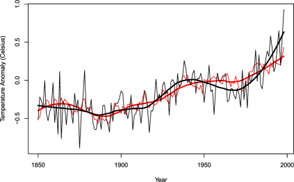
Figure 15: In-sample Backcast from Bayesian Model of Section 5. CRU Northern Hemisphere annual mean land temperature is given by the thin black line and a smoothed version is given by the thick black line. The backcast is given by the thin red line and a smoothed version is given by the thick red line. The model is fit on 1850–1998 AD.

We plot the in-sample portion of this backcast (1850–1998 AD) in Figure 15. Not surprisingly, the model tracks CRU reasonably well because it is in-sample. However, despite the fact that the backcast is both in-sample and initialized with the high true temperatures from 1999 AD and 2000 AD, it still cannot capture either the high level of or the sharp run-up in temperatures of the 1990s: it is substantially biased low. That the model cannot capture run-up even in-sample does not portend well for its ability to capture similar levels and run-ups if they exist out-of-sample.

A benefit of our fully Bayesian model is that it allows us to assess the error due to both (i) residual variance (i.e., $\varepsilon_{t}$) and (ii) parameter uncertainty. Furthermore, we can do this in a fully pathwise fashion. To assess the error due to residual variance, we use the one-step-behind backcasting procedure outlined above with two exceptions. First, at each step, we draw an error from a $N(0,\sigma^{2})$ distribution and add it to our backcast. These errors then propagate through the full path of backcast. Second, we perform the backcast allowing $\sigma$ to vary over our samples from the posterior distribution.

To assess the error due to the uncertainty in $\vec{\beta}$, we perform the original one-step-behind backcast [i.e., without drawing an error from the $N(0,\sigma^{2})$ distribution]. However, rather than using the posterior mean of $\vec{\beta}$, we perform the backcast for each of our samples from the posterior distribution of $\vec{\beta}$.

Finally, to get a sense of the full uncertainty in our backcast, we can combine both of the methods outlined above. That is, for each draw from the posterior of $\vec{\beta}$ and $\sigma$, we perform the one-step-behind backcast drawing errors from the $N(0,\sigma^{2})$ distribution. This gives one curve for each posterior draw, each representing a draw of the full temperature series conditional on the data and the model. Taken together, they form an approximation to the full posterior distribution of the temperature series.

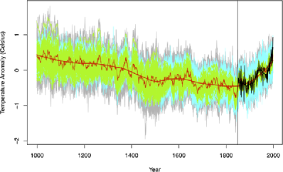
Figure 16: Backcast from Bayesian Model of Section 5. CRU Northern Hemisphere annual mean land temperature is given by the thin black line and a smoothed version is given by the thick black line. The forecast is given by the thin red line and a smoothed version is given by the thick red line. The model is fit on 1850–1998 AD and backcasts 998–1849 AD. The cyan region indicates uncertainty due to $\varepsilon_{t}$, the green region indicates uncertainty due to $\vec{\beta}$, and the gray region indicates total uncertainty.

We decompose the uncertainty of our model’s backcast by plotting the curves drawn using each of the methods outlined in the previous three paragraphs in Figure 16. As can be seen, in the modern instrumental period the residual variance (in cyan) dominates the uncertainty in the backcast. However, the variance due to $\vec{\beta}$ uncertainty (in green) propagates through time and becomes the dominant portion of the overall error for earlier periods. The primary conclusion is that failure to account for parameter uncertainty results in overly confident model predictions.

As far as we can tell, no effort at paleoclimatological global temperature reconstruction of the past 1000 years has used a fully Bayesian probability model to incorporate parameter uncertainty into the backcast estimates [in fact, the aforementioned Li, Nychka and Amman (2007) paper is the only paper we know of that even begins to account for uncertainty in some of the parameters; see Haslett et al. (2006) for a Bayesian model used for reconstructing the local prehistoric climate in Glendalough, Ireland]. The widely used approach in the climate literature is to estimate uncertainty using residuals (usually from a holdout period). Climate scientist generally report less accurate reconstructions in more distant time periods, but this is due to the fact that there are fewer proxies that extend further back into time and therefore larger validation residuals.

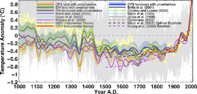
Figure 17: This figure modifies Figure $3$ from Mann et al. (2008). We take that figure and superimpose the backcast from Bayesian model of Section 5. The backcast is given by the thin yellow line, the smoothed backcast by a thick yellow line, and the backcast error in gray.

5.4 Comparison to other reconstructions and posterior calculations

What is most interesting is comparing our backcast to those from Mann et al. (2008) as done in Figure 17. We see that our model gives a backcast which is very similar to those in the literature, particularly from 1300 AD to the present. In fact, our backcast very closely traces the Mann et al. (2008) EIV land backcast, considered by climate scientists to be among the most skilled. Though our model provides slightly warmer backcasts for the years 1000–1300 AD, we note it falls within or just outside the uncertainty bands of the Mann et al. (2008) EIV land backcast even in that period. Hence, our backcast matches their backcasts reasonably well.

The major difference between our model and those of climate scientists, however, can be seen in the large width of our uncertainty bands. Because they are pathwise and account for the uncertainty in the parameters (as outlined in Section 5.3), they are much larger than those provided by climate scientists. In fact, our uncertainty bands are so wide that they envelop all of the other backcasts in the literature. Given their ample width, it is difficult to say that recent warming is an extraordinary event compared to the last 1000 years. For example, according to our uncertainty bands, it is possible that it was as warm in the year 1200 AD as it is today. In contrast, the reconstructions produced in Mann et al. (2008) are completely pointwise.

Another advantage of our method is that it allows us to calculate posterior probabilities of various scenarios of interest by simulation of alternative sample paths. For example, 1998 is generally considered to be the warmest year on record in the Northern Hemisphere. Using our model, we calculate that there is a 36% posterior probability that 1998 was the warmest year over the past thousand. If we consider rolling decades, 1997–2006 is the warmest on record; our model gives an 80% chance that it was the warmest in the past 1000 years. Finally, if we look at rolling 30-year blocks, the posterior probability that the last 30 years (again, the warmest on record) were the warmest over the past thousand is 38%.

Similarly, we can look at posterior probabilities of the run-up in (or derivative of) temperatures in addition to the levels. For this purpose, we defined the “derivative” as the difference between the value of the loess smooth of the temperature series (or reconstruction series) in year $t$ and year $t-k$. For $k=10$, $k=30$, and $k=60$, we estimate a zero posterior probability that the past 1000 years contained run-ups larger than those we have experienced over the past ten, 30, and 60 years (again, the largest such run-ups on record). This suggests that the temperature derivatives encountered over recent history are unprecedented in the millennium. While this does seem alarming, we should temper our alarm somewhat by considering again Figure 15 and the fact that the proxies seem unable to capture the sharp run-up in temperature of the 1990s. That is, our posterior probabilities are based on derivatives from our model’s proxy-based reconstructions and we are comparing these derivatives to derivatives of the actual temperature series; insofar as the proxies cannot capture sharp run-ups, our model’s reconstructions will not be able to either and therefore will tend to understate the probability of such run-ups.

5.5 Model validation

Though our model gives forecasts and backcasts that are broadly comparable to those provided by climate scientists, our approach suggests that there is substantial uncertainty about the ability of the model to fit and predict new data. Climate scientists estimate out-of-sample uncertainty using only two holdout blocks: one at the beginning of the instrumental period and one at the end. We pursue that strategy here. First, we fit on 1880–1998 AD and attempt to backcast 1850–1879 AD. Then, we fit on 1850–1968 AD and forecast 1969–1998 AD. These blocks are arguably the most interesting and important because they are not “tied” at two endpoints. Thus, they genuinely reflect the most important modeling task: reconstruction.

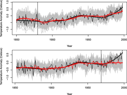
Figure 18: Predictions from the Bayesian model of Section 5 when the first $30$ years of instrumental data are held out (top) and when the last $30$ years of instrumental data are held out (bottom). CRU is given in black and the model predictions in red. The raw data and predictions are given by the thin lines and loess smooths are given by the thick lines. Uncertainty bands are indicated by the gray region.

Figure 18 illustrates that the model seems to perform reasonably well on the first holdout block. Our reconstruction regresses partly back toward the in-sample mean. Compared to the actual temperature series, it is biased a bit upward. On the other hand, the model is far more inaccurate on the second holdout block, the modern period. Our reconstruction, happily, does not move toward the in-sample mean and even rises substantively at first. Still, it seems there is simply not enough signal in the proxies to detect either the high levels of or the sharp run-up in temperature seen in the 1990s. This is disturbing: if a model cannot predict the occurrence of a sharp run-up in an out-of-sample block which is contiguous with the in-sample training set, then it seems highly unlikely that it has power to detect such levels or run-ups in the more distant past. It is even more discouraging when one recalls Figure 15: the model cannot capture the sharp run-up even in-sample. In sum, these results suggest that the 93 sequences that comprise the 1000-year-old proxy record simply lack power to detect a sharp increase in temperature.

As mentioned earlier, scientists have collected a large body of evidence which suggests that there was a Medieval Warm Period (MWP) at least in portions of the Northern Hemisphere. The MWP is believed to have occurred c. 800–1300 AD (it was followed by the Little Ice Age). It is widely hoped that multi-proxy models have the power to detect (i) how warm the Medieval Warm Period was, (ii) how sharply temperatures increased during it, and (iii) to compare these two features to the past decade’s high temperatures and sharp run-up. Since our model cannot detect the recent temperature change, detection of dramatic changes hundreds of years ago seems out of the question.

This is not to say that the proxy record is unrelated to temperatures. We can compare our model’s RMSE in these two holdout periods to various null models which we know have no signal. That is, we can perform a test similar to that of Section 3.4. On each holdout block, we generate a $149\times 93$ matrix of pseudo-proxies from each of the six null models known to be independent of the temperature series. Then, analogously to our model, we take the first ten principal components of these pseudo-proxies, regress the in-sample temperature on the ten in-sample principal components, and compute the RMSE on the holdout block. We perform this procedure 1000 times for each holdout block and then calculate the percentage of time that the model fit to the pseudo-proxies beats our model.

=290pt Pseudo-proxy First block $\bolds{p}$-value Last block $\bolds{p}$-value White Noise 00.0% 00.0% AR1(0.25) 00.1% 00.0% AR1(0.4) 00.1% 00.0% Empirical AR1 24.1% 20.6% Brownian Motion 16.4% 32.2%

Table 2: Percent of time various null models outperform the Bayesian model of Section 5

Our model, with an RMSE of 0.26 on the first holdout block and an RMSE of 0.36 on the second handily outperforms the relatively unsophisticated white noise and weak AR1 process pseudo-proxies (see Table 2). Again, this is not surprising. These pseudo-proxies cannot capture the local dependence in the instrumental record, so they regress sharply to the in-sample mean. On the other hand, the Empirical AR1 processes and Brownian motion have more complex local structure so they provide respectable competition to our model. These models capture only the local dependence in the temperature record: in the long term, forecasts based off the AR1 processes will slide slowly back to the in-sample mean and forecasts based off Brownian motion will wander aimlessly. Taken together, it follows that our model is at best weakly significant relative to the Empirical AR1 process or Brownian motion on either holdout block.

In tandem, Figure 18 and Table 2 should make us very cautious about using our model to extrapolate, even with wide standard errors. The second panel of Figure 18 demonstrates that these standard errors are too narrow even for very temporally short forecasts. While we are able to replicate the significance tests in Mann, Bradley and Hughes (1998), our Table 2 shows that our model does not pass “statistical significance” thresholds against savvy null models. Ultimately, what these tests essentially show is that the 1000-year-old proxy record has little power given the limited temperature record.

6 Conclusion

Research on multi-proxy temperature reconstructions of the earth’s temperature is now entering its second decade. While the literature is large, there has been very little collaboration with university-level, professional statisticians [Wegman, Scott and Said (2006), Wegman (2006)]. Our paper is an effort to apply some modern statistical methods to these problems. While our results agree with the climate scientists findings in some respects, our methods of estimating model uncertainty and accuracy are in sharp disagreement.

On the one hand, we conclude unequivocally that the evidence for a “long-handled” hockey stick (where the shaft of the hockey stick extends to the year 1000 AD) is lacking in the data. The fundamental problem is that there is a limited amount of proxy data which dates back to 1000 AD; what is available is weakly predictive of global annual temperature. Our backcasting methods, which track quite closely the methods applied most recently in Mann (2008) to the same data, are unable to catch the sharp run up in temperatures recorded in the 1990s, even in-sample. As can be seen in Figure 15, our estimate of the run up in temperature in the 1990s has a much smaller slope than the actual temperature series. Furthermore, the lower frame of Figure 18 clearly reveals that the proxy model is not at all able to track the high gradient segment. Consequently, the long flat handle of the hockey stick is best understood to be a feature of regression and less a reflection of our knowledge of the truth. Nevertheless, the temperatures of the last few decades have been relatively warm compared to many of the 1000-year temperature curves sampled from the posterior distribution of our model.

Our main contribution is our efforts to seriously grapple with the uncertainty involved in paleoclimatological reconstructions. Regression of high-dimensional time series is always a complex problem with many traps. In our case, the particular challenges include (i) a short sequence of training data, (ii) more predictors than observations, (iii) a very weak signal, and (iv) response and predictor variables which are both strongly autocorrelated. The final point is particularly troublesome: since the data is not easily modeled by a simple autoregressive process, it follows that the number of truly independent observations (i.e., the effective sample size) may be just too small for accurate reconstruction.

Climate scientists have greatly underestimated the uncertainty of proxy-based reconstructions and hence have been overconfident in their models. We have shown that time dependence in the temperature series is sufficiently strong to permit complex sequences of random numbers to forecast out-of-sample reasonably well fairly frequently (see Figures 9 and 10). Furthermore, even proxy-based models with approximately the same amount of reconstructive skill (Figures 11–13), produce strikingly dissimilar historical backcasts (Figure 14); some of these look like hockey sticks but most do not.

Natural climate variability is not well understood and is probably quite large. It is not clear that the proxies currently used to predict temperature are even predictive of it at the scale of several decades let alone over many centuries. Nonetheless, paleoclimatoligical reconstructions constitute only one source of evidence in the AGW debate.

Our work stands entirely on the shoulders of those environmental scientists who labored untold years to assemble the vast network of natural proxies. Although we assume the reliability of their data for our purposes here, there still remains a considerable number of outstanding questions that can only be answered with a free and open inquiry and a great deal of replication.

References

- Amman et al. (2007) {barticle}[auto:STB—2010-11-18—09:18:59] \bauthor\bsnmAmman, \bfnmC. M.\binitsC. M., \bauthor\bsnmJoos, \bfnmF.\binitsF., \bauthor\bsnmOtto-Bliesner, \bfnmB. L.\binitsB. L. and \bauthor\bsnmTomas, \bfnmR.\binitsR. (\byear2007). \btitleSolar influence on climate during the past millennium: Results from transient simulations with the NCAR climate system model. \bjournalProc. Natl. Acad. Sci. USA \bvolume104 \bpages3713–3718. \endbibitem
- Ammann and Wahl (2007) {barticle}[auto:STB—2010-11-18—09:18:59] \bauthor\bsnmAmmann, \bfnmC.\binitsC. and \bauthor\bsnmWahl, \bfnmE.\binitsE. (\byear2007). \btitleThe importance of the geophysical context in statistical evaluations of climate reconstruction procedures. \bjournalClimatic Change \bvolume85 \bpages71–88. \endbibitem
- BBC (2008) {bmisc}[auto:STB—2010-11-18—09:18:59] \borganizationBBC (\byear2008). \bhowpublishedEarth: The Climate Wars. British Broadcasting Company, September 14. \endbibitem
- Bradley (1999) {bbook}[auto:STB—2010-11-18—09:18:59] \bauthor\bsnmBradley, \bfnmR. S.\binitsR. S. (\byear1999). \btitlePaleoclimatology: Reconstructing Climates of the Quaternary, \bedition2nd ed. \bpublisherAcademic Press, \baddressSan Diego. \endbibitem
- Christiansen, Schmith and Thejll (2009) {barticle}[auto:STB—2010-11-18—09:18:59] \bauthor\bsnmChristiansen, \bfnmB.\binitsB., \bauthor\bsnmSchmith, \bfnmT.\binitsT. and \bauthor\bsnmThejll, \bfnmP.\binitsP. (\byear2009). \btitleA surrogate emsemble study of climate reconstruction methods: Stochasticity and robustness. \bjournalJournal of Climate \bvolume22 \bpages951–976. \endbibitem
- Gore (2006) {bmisc}[auto:STB—2010-11-18—09:18:59] \bauthor\bsnmGore, \bfnmA.\binitsA. (\byear2006). \bhowpublishedAn Inconvenient Truth. Lawrence Bender Productions. \endbibitem
- Granger and Newbold (1974) {barticle}[auto:STB—2010-11-18—09:18:59] \bauthor\bsnmGranger, \bfnmC. W. J.\binitsC. W. J. and \bauthor\bsnmNewbold, \bfnmP.\binitsP. (\byear1974). \btitleSpurious regressions in econometrics. \bjournalJournal of Econometrics \bvolume2 \bpages111–120. \endbibitem
- Green, Armstrong and Soon (2009) {barticle}[auto:STB—2010-11-18—09:18:59] \bauthor\bsnmGreen, \bfnmK. C.\binitsK. C., \bauthor\bsnmArmstrong, \bfnmJ. S.\binitsJ. S. and \bauthor\bsnmSoon, \bfnmW.\binitsW. (\byear2009). \btitleValidity of climate change forecasting for public policy decision-making. \bjournalInternational Journal of Forecasting \bvolume25 \bpages826–832. \endbibitem
- Haslett et al. (2006) {barticle}[mr] \bauthor\bsnmHaslett, \bfnmJ.\binitsJ., \bauthor\bsnmWhiley, \bfnmM.\binitsM., \bauthor\bsnmBhattacharya, \bfnmS.\binitsS., \bauthor\bsnmSalter-Townshend, \bfnmM.\binitsM., \bauthor\bsnmWilson, \bfnmSimon P.\binitsS. P., \bauthor\bsnmAllen, \bfnmJ. R. M.\binitsJ. R. M., \bauthor\bsnmHuntley, \bfnmB.\binitsB. and \bauthor\bsnmMitchell, \bfnmF. J. G.\binitsF. J. G. (\byear2006). \btitleBayesian palaeoclimate reconstruction. \bjournalJ. Roy. Statist. Soc. Ser. A \bvolume169 \bpages395–438. \biddoi=10.1111/j.1467-985X.2006.00429.x, mr=2236914 \endbibitem
- IPCC (2001) {bmisc}[auto:STB—2010-11-18—09:18:59] \borganizationIPCC (\byear2001). \bhowpublishedClimate Change 2001: The Scientific Basis. Cambridge Univ. Press, Cambridge. \endbibitem
- IPCC (2007) {bmisc}[auto:STB—2010-11-18—09:18:59] \borganizationIPCC (\byear2007). \bhowpublishedClimate Change 2007: The Physical Science Basis. Contribution of Working Group I to the Fourth Assessment Report of the Intergovernmental Panel on Climate Change. \endbibitem
- Johnson (2009) {bmisc}[auto:STB—2010-11-18—09:18:59] \bauthor\bsnmJohnson, \bfnmK.\binitsK. (\byear2009). \bhowpublishedClimate emails stoke debate. Wall Street Journal. November 23, page A3. \endbibitem
- Johnson and Naik (2009) {bmisc}[auto:STB—2010-11-18—09:18:59] \bauthor\bsnmJohnson, \bfnmK.\binitsK. and \bauthor\bsnmNaik, \bfnmG.\binitsG. (\byear2009). \bhowpublishedLawmakers probe climate emails. Wall Street Journal. November 24, page A8. \endbibitem
- Jolis (2009) {bmisc}[auto:STB—2010-11-18—09:18:59] \bauthor\bsnmJolis, \bfnmA.\binitsA. (\byear2009). \bhowpublishedRevenge of the climate laymen. Wall Street Journal. November 18. \endbibitem
- Ladurie (1971) {bbook}[auto:STB—2010-11-18—09:18:59] \bauthor\bsnmLadurie, \bfnmE. L.\binitsE. L. (\byear1971). \btitleTimes of Feast, Times of Famine: A History of Climate Since the Year 1000. \bpublisherDoubleday, \baddressNew York. \endbibitem
- Lamb (1990) {bbook}[auto:STB—2010-11-18—09:18:59] \bauthor\bsnmLamb, \bfnmH. H.\binitsH. H. (\byear1990). \btitleClimate: Past, Present and Future. \bpublisherRoutledge, \baddressNew York. \endbibitem
- Lee, Zwiers and Tsao (2008) {barticle}[auto:STB—2010-11-18—09:18:59] \bauthor\bsnmLee, \bfnmT.\binitsT., \bauthor\bsnmZwiers, \bfnmF. W.\binitsF. W. and \bauthor\bsnmTsao, \bfnmM.\binitsM. (\byear2008). \btitleEvaluation of proxy-based millennial reconstruction methods. \bjournalClimate Dynamics \bvolume31 \bpages263–281. \endbibitem
- Li, Nychka and Amman (2007) {barticle}[auto:STB—2010-11-18—09:18:59] \bauthor\bsnmLi, \bfnmB.\binitsB., \bauthor\bsnmNychka, \bfnmD. W.\binitsD. W. and \bauthor\bsnmAmman, \bfnmC. M.\binitsC. M. (\byear2007). \btitleThe ‘hockey stick’ and the 1990s: A statistical perspective on reconstructing hemispheric temperatures. \bjournalTellus \bvolume59A \bpages591–598. \endbibitem
- Li, Nychka and Amman (2010) {barticle}[auto:STB—2010-11-18—09:18:59] \bauthor\bsnmLi, \bfnmB.\binitsB., \bauthor\bsnmNychka, \bfnmD. W.\binitsD. W. and \bauthor\bsnmAmman, \bfnmC. M.\binitsC. M. (\byear2010). \btitleThe value of multi-proxy reconstructin of past climate. \bjournalJ. Amer. Statist. Assoc. \bvolume105 \bpages883–895. \endbibitem
- Luterbacher et al. (2004) {barticle}[auto:STB—2010-11-18—09:18:59] \bauthor\bsnmLuterbacher, \bfnmJ.\binitsJ., \bauthor\bsnmDieterich, \bfnmD.\binitsD., \bauthor\bsnmXoplaki, \bfnmE.\binitsE., \bauthor\bsnmGrosjean, \bfnmM.\binitsM. and \bauthor\bsnmWanner, \bfnmH.\binitsH. (\byear2004). \btitleEuropean seasonal and annual temperature variability, trends, and extremes since 1500. \bjournalScience \bvolume202 \bpages1499–1503. \endbibitem
- Mann (2004) {barticle}[auto:STB—2010-11-18—09:18:59] \bauthor\bsnmMann, \bfnmM. E.\binitsM. E. (\byear2004). \btitleOn smoothing potentially non-stationary climate time series. \bjournalGeophysical Research Letters \bvolume31. \endbibitem
- Mann (2008) {barticle}[auto:STB—2010-11-18—09:18:59] \bauthor\bsnmMann, \bfnmM. E.\binitsM. E. (\byear2008). \btitleSmoothing of climate time series revisited. \bjournalGeophysical Research Letters \bvolume35. \endbibitem
- Mann, Bradley and Hughes (1998) {barticle}[auto:STB—2010-11-18—09:18:59] \bauthor\bsnmMann, \bfnmM. E.\binitsM. E., \bauthor\bsnmBradley, \bfnmR. E.\binitsR. E. and \bauthor\bsnmHughes, \bfnmM. K.\binitsM. K. (\byear1998). \btitleGlobal-scale temperature patterns and climate forcing over the past six centuries. \bjournalNature \bvolume392 \bpages779–787. \endbibitem
- Mann, Bradley and Hughes (1999) {barticle}[auto:STB—2010-11-18—09:18:59] \bauthor\bsnmMann, \bfnmM. E.\binitsM. E., \bauthor\bsnmBradley, \bfnmR. E.\binitsR. E. and \bauthor\bsnmHughes, \bfnmM. K.\binitsM. K. (\byear1999). \btitleNorthern hemisphere temperatures during the past millennium: Inferences, uncertainties, and limitations. \bjournalGeophysical Research Letters \bvolume26 \bpages759–762. \endbibitem
- Mann, Bradley and Hughes (2004) {barticle}[auto:STB—2010-11-18—09:18:59] \bauthor\bsnmMann, \bfnmM. E.\binitsM. E., \bauthor\bsnmBradley, \bfnmR. E.\binitsR. E. and \bauthor\bsnmHughes, \bfnmM. K.\binitsM. K. (\byear2004). \btitleCorrigendum: Global-scale temperature patterns and climate forcing over the past six centuries. \bjournalNature \bvolume430 \bpages105. \endbibitem
- Mann and Rutherford (2002) {barticle}[auto:STB—2010-11-18—09:18:59] \bauthor\bsnmMann, \bfnmM. E.\binitsM. E. and \bauthor\bsnmRutherford, \bfnmS.\binitsS. (\byear2002). \btitleClimate reconstruction using pseudoproxies. \bjournalGeophysical Research Letters \bvolume29 \bpages1501. \endbibitem
- Mann et al. (2005) {barticle}[auto:STB—2010-11-18—09:18:59] \bauthor\bsnmMann, \bfnmM. E.\binitsM. E., \bauthor\bsnmRutherford, \bfnmS.\binitsS., \bauthor\bsnmWahl, \bfnmE.\binitsE. and \bauthor\bsnmAmmann, \bfnmC.\binitsC. (\byear2005). \btitleTesting the fidelity of methods used in proxy-based reconstructions of past climate. \bjournalJournal of Climate \bvolume18 \bpages4097–4107. \endbibitem
- Mann et al. (2007) {barticle}[auto:STB—2010-11-18—09:18:59] \bauthor\bsnmMann, \bfnmM. E.\binitsM. E., \bauthor\bsnmRutherford, \bfnmS.\binitsS., \bauthor\bsnmWahl, \bfnmE.\binitsE. and \bauthor\bsnmAmmann, \bfnmC.\binitsC. (\byear2007). \btitleRobustness of proxy-based climate field reconstruction methods. \bjournalJournal of Geophysical Research \bvolume112. \endbibitem
- Mann et al. (2008) {barticle}[auto:STB—2010-11-18—09:18:59] \bauthor\bsnmMann, \bfnmM. E.\binitsM. E., \bauthor\bsnmZhang, \bfnmZ.\binitsZ., \bauthor\bsnmHughes, \bfnmM. K.\binitsM. K., \bauthor\bsnmBradley, \bfnmR. S.\binitsR. S., \bauthor\bsnmMiller, \bfnmS. K.\binitsS. K., \bauthor\bsnmRutherford, \bfnmS.\binitsS. and \bauthor\bsnmNi, \bfnmF.\binitsF. (\byear2008). \btitleProxy-based reconstructions of hemispheric and global surface temperature variations over the past two millenia. \bjournalProc. Natl. Acad. Sci. USA \bvolume105 \bpages13252–13257. \endbibitem
- Matthes (1939) {barticle}[auto:STB—2010-11-18—09:18:59] \bauthor\bsnmMatthes, \bfnmF. E.\binitsF. E. (\byear1939). \btitleReport of the committee on glaciers. \bjournalTransactions of the American Geophysical Union \bvolume20 \bpages518–523. \endbibitem
- McIntyre and McKitrick (2003) {barticle}[auto:STB—2010-11-18—09:18:59] \bauthor\bsnmMcIntyre, \bfnmS.\binitsS. and \bauthor\bsnmMcKitrick, \bfnmR.\binitsR. (\byear2003). \btitleCorrections to the Mann et al. (1998) proxy base and northern hemispheric average temperature series. \bjournalEnergy and Environment \bvolume14 \bpages751–771. \endbibitem
- McIntyre and McKitrick (2005a) {barticle}[auto:STB—2010-11-18—09:18:59] \bauthor\bsnmMcIntyre, \bfnmS.\binitsS. and \bauthor\bsnmMcKitrick, \bfnmR.\binitsR. (\byear2005a). \btitleHockey sticks, principal components, and spurious significance. \bjournalGeophysical Research Letters \bvolume32. \endbibitem
- McIntyre and McKitrick (2005b) {barticle}[auto:STB—2010-11-18—09:18:59] \bauthor\bsnmMcIntyre, \bfnmS.\binitsS. and \bauthor\bsnmMcKitrick, \bfnmR.\binitsR. (\byear2005b). \btitleThe M&M critique of the MBH98 and northern hemisphere climate index: Update and implications. \bjournalEnergy and Environment \bvolume16 \bpages69–100. \endbibitem
- McIntyre and McKitrick (2005c) {barticle}[auto:STB—2010-11-18—09:18:59] \bauthor\bsnmMcIntyre, \bfnmS.\binitsS. and \bauthor\bsnmMcKitrick, \bfnmR.\binitsR. (\byear2005c). \btitleReply to comment by Huybers on “Hockey sticks, principal components, and spurious significance.” \bjournalGeophysical Research Letters \bvolume32 \bpagesL20713. \endbibitem
- McShane and Wyner (2011) {bmisc}[auto:STB—2010-11-18—09:18:59] \bauthor\bsnmMcShane, \bfnmB. B.\binitsB. B. and \bauthor\bsnmWyner, \bfnmA. J.\binitsA. J. (\byear2011). \bhowpublishedSupplement to: “A statistical analysis of multiple temperature proxies: Are reconstructions of surface temperatures over the last 1000 years reliable?” DOI: 10.1214/10-AOAS398SUPP. \endbibitem
- NRC (2006) {bmisc}[auto:STB—2010-11-18—09:18:59] \borganizationNational Research Council (\byear2006). \bhowpublishedSurface temperature reconstructions. National Academic Press, Washington, DC. \endbibitem
- Phillips (1986) {barticle}[mr] \bauthor\bsnmPhillips, \bfnmP. C. B.\binitsP. C. B. (\byear1986). \btitleUnderstanding spurious regressions in econometrics. \bjournalJ. Econometrics \bvolume33 \bpages311–340. \biddoi=10.1016/0304-4076(86)90001-1, mr=0867979 \endbibitem
- Rothstein (2008) {barticle}[auto:STB—2010-11-18—09:18:59] \bauthor\bsnmRothstein, \bfnmE.\binitsE. (\byear2008). \btitleApocalypse now, via diorama. \bjournalThe New York Times. \bnoteOctober 17, page C27. \endbibitem
- Rutherford et al. (2005) {barticle}[auto:STB—2010-11-18—09:18:59] \bauthor\bsnmRutherford, \bfnmS.\binitsS., \bauthor\bsnmMann, \bfnmM. E.\binitsM. E., \bauthor\bsnmOsborn, \bfnmT. J.\binitsT. J., \bauthor\bsnmBradley, \bfnmR. S.\binitsR. S., \bauthor\bsnmBriffa, \bfnmK. R.\binitsK. R., \bauthor\bsnmHughes, \bfnmM. K.\binitsM. K. and \bauthor\bsnmJones, \bfnmP. D.\binitsP. D. (\byear2005). \btitleProxy-based northern hemispheric surface reconstructions: Sensitivity to method, predictor network, target season, and target domain. \bjournalJournal of Climate \bvolume18 \bpages2308–2329. \endbibitem
- Schneider (2001) {barticle}[auto:STB—2010-11-18—09:18:59] \bauthor\bsnmSchneider, \bfnmT.\binitsT. (\byear2001). \btitleAnalysis of incomplete climate data: Estimation of mean values and covariance matrices and imputation of missing values. \bjournalJournal of Climate \bvolume14 \bpages853–871. \endbibitem
- Tibshirani (1996) {barticle}[mr] \bauthor\bsnmTibshirani, \bfnmRobert\binitsR. (\byear1996). \btitleRegression shrinkage and selection via the lasso. \bjournalJ. Roy. Statist. Soc. Ser. B \bvolume58 \bpages267–288. \bidmr=1379242 \endbibitem
- Tingley and Huybers (2010a) {barticle}[auto:STB—2010-11-18—09:18:59] \bauthor\bsnmTingley, \bfnmM.\binitsM. and \bauthor\bsnmHuybers, \bfnmP.\binitsP. (\byear2010a). \btitleA Bayesian algorithm for reconstructing climate anomalies in space and time. Part I: Development and applications to paleoclimate reconstruction problems. \bjournalJournal of Climate \bvolume23 \bpages2759–2781. \endbibitem
- Tingley and Huybers (2010b) {barticle}[auto:STB—2010-11-18—09:18:59] \bauthor\bsnmTingley, \bfnmM.\binitsM. and \bauthor\bsnmHuybers, \bfnmP.\binitsP. (\byear2010b). \btitleBayesian algorithm for reconstructing climate anomalies in space and time. Part II: Comparison with the regularized expectation–maximization algorithm. \bjournalJournal of Climate \bvolume23 \bpages2782–2800. \endbibitem
- von Storch and Zorita (2005) {barticle}[auto:STB—2010-11-18—09:18:59] \bauthor\bparticlevon \bsnmStorch, \bfnmH. E.\binitsH. E. and \bauthor\bsnmZorita, \bfnmE.\binitsE. (\byear2005). \btitleComment on “Hockey sticks, principal components, and spurious significance,” by S. McIntyre and R. McKitrick. \bjournalGeophysical Research Letters \bvolume32. \endbibitem
- von Storch et al. (2004) {barticle}[auto:STB—2010-11-18—09:18:59] \bauthor\bparticlevon \bsnmStorch, \bfnmH. E.\binitsH. E., \bauthor\bsnmZorita, \bfnmE.\binitsE., \bauthor\bsnmJones, \bfnmJ. M.\binitsJ. M., \bauthor\bsnmDimitriev, \bfnmY.\binitsY., \bauthor\bsnmGonzalez-Rouco, \bfnmF.\binitsF. and \bauthor\bsnmTett, \bfnmS.\binitsS. (\byear2004). \btitleReconstructing past climate from noisy data. \bjournalScience \bvolume306 \bpages679–682. \endbibitem
- von Storch et al. (2006) {barticle}[auto:STB—2010-11-18—09:18:59] \bauthor\bparticlevon \bsnmStorch, \bfnmH. E.\binitsH. E., \bauthor\bsnmZorita, \bfnmE.\binitsE., \bauthor\bsnmJones, \bfnmJ. M.\binitsJ. M., \bauthor\bsnmDimitriev, \bfnmY.\binitsY., \bauthor\bsnmGonzalez-Rouco, \bfnmF.\binitsF. and \bauthor\bsnmTett, \bfnmS.\binitsS. (\byear2006). \btitleResponse to comment on “Reconstructing past climate from noisy data.” \bjournalScience \bvolume213 \bpages529. \endbibitem
- Wahl and Amman (2006) {barticle}[auto:STB—2010-11-18—09:18:59] \bauthor\bsnmWahl, \bfnmE. R.\binitsE. R. and \bauthor\bsnmAmman, \bfnmC. M.\binitsC. M. (\byear2006). \btitleRobustness of the Mann, Bradley, Hughes reconstruction of the Northern Hemisphere surface temperatures: Examination of criticisms based on the nature and processing of proxy climate evidence. \bjournalClimatic Change \bvolume85 \bpages33–69. \endbibitem
- Wahl, Ritson and Amman (2006) {barticle}[auto:STB—2010-11-18—09:18:59] \bauthor\bsnmWahl, \bfnmE. R.\binitsE. R., \bauthor\bsnmRitson, \bfnmD. M.\binitsD. M. and \bauthor\bsnmAmman, \bfnmC. M.\binitsC. M. (\byear2006). \btitleOn “Reconstruction past climate from noisy data.” \bjournalScience \bvolume312 \bpages592b. \endbibitem
- Wegman (2006) {bmisc}[auto:STB—2010-11-18—09:18:59] \bauthor\bsnmWegman, \bfnmE. J.\binitsE. J. (\byear2006). \bhowpublished\btitleResponse of Dr. Edward Wegman to questions posed by the honorable Bart Stupak in connection with testimony to the subcommittee on oversight and investigations. Available at http://www.uoguelph.ca/~rmckitri/research/StupakResponse.pdf. \endbibitem
- Wegman, Scott and Said (2006) {bmisc}[auto:STB—2010-11-18—09:18:59] \bauthor\bsnmWegman, \bfnmE. J.\binitsE. J., \bauthor\bsnmScott, \bfnmD. W.\binitsD. W. and \bauthor\bsnmSaid, \bfnmY. H.\binitsY. H. (\byear2006). \bhowpublished\btitleAd Hoc committee report on the ‘hockey stick’ global climate reconstruction. Available at http://republicans.energycommerce.house.gov/108/home/07142006_Wegman_Report.pdf. \endbibitem
- Wu, Boos and Stefanski (2007) {barticle}[mr] \bauthor\bsnmWu, \bfnmYujun\binitsY., \bauthor\bsnmBoos, \bfnmDennis D.\binitsD. D. and \bauthor\bsnmStefanski, \bfnmLeonard A.\binitsL. A. (\byear2007). \btitleControlling variable selection by the addition of pseudovariables. \bjournalJ. Amer. Statist. Assoc. \bvolume102 \bpages235–243. \biddoi=10.1198/016214506000000843, mr=2345541 \endbibitem
- Yule (1926) {barticle}[auto:STB—2010-11-18—09:18:59] \bauthor\bsnmYule, \bfnmG. U.\binitsG. U. (\byear1926). \btitleWhy do we sometimes get nonsense correlations between time series? A study in sampling and the nature of time series. \bjournalJ. Roy. Statist. Soc. \bvolume89 \bpages1–64. \endbibitem